www.hydrol-earth-syst-sci.net/18/4791/2014/ doi:10.5194/hess-18-4791-2014
© Author(s) 2014. CC Attribution 3.0 License.
High-resolution land surface modeling utilizing remote
sensing parameters and the Noah UCM: a case study in the
Los Angeles Basin
P. Vahmani1and T. S. Hogue1,2
1University of California, Los Angeles, CA, USA 2Colorado School of Mines, Golden, CO, USA Correspondence to: T. S. Hogue ([email protected])
Received: 27 April 2014 – Published in Hydrol. Earth Syst. Sci. Discuss.: 4 July 2014 Revised: – – Accepted: 25 October – Published: 3 December 2014
Abstract. In the current work we investigate the utility of remote-sensing-based surface parameters in the Noah UCM (urban canopy model) over a highly developed urban area. Landsat and fused Landsat–MODIS data are utilized to gen-erate high-resolution (30 m) monthly spatial maps of green vegetation fraction (GVF), impervious surface area (ISA), albedo, leaf area index (LAI), and emissivity in the Los An-geles metropolitan area. The gridded remotely sensed param-eter data sets are directly substituted for the land-use/lookup-table-based values in the Noah-UCM modeling framework. Model performance in reproducing ET (evapotranspiration) and LST (land surface temperature) fields is evaluated uti-lizing Landsat-based LST and ET estimates from CIMIS (California Irrigation Management Information System) sta-tions as well as in situ measurements. Our assessment shows that the large deviations between the spatial distributions and seasonal fluctuations of the default and measured pa-rameter sets lead to significant errors in the model predic-tions of monthly ET fields (RMSE=22.06 mm month−1). Results indicate that implemented satellite-derived parameter maps, particularly GVF, enhance the capability of the Noah UCM to reproduce observed ET patterns over vegetated areas in the urban domains (RMSE=11.77 mm month−1). GVF plays the most significant role in reproducing the observed ET fields, likely due to the interaction with other parameters in the model. Our analysis also shows that remotely sensed GVF and ISA improve the model’s capability to predict the LST differences between fully vegetated pixels and highly developed areas.
1 Introduction
Urbanization introduces significant changes to land sur-face characteristics that ultimately perturb land–atmosphere fluxes of sensible heat, latent heat, and momentum which, in turn, alter atmospheric properties as well as local weather and climate (Landsberg, 1981; Kalnay and Cai, 2003; Miao et al., 2009; De Ridder et al., 2012). Urban surfaces are covered with variety of materials with distinct thermal, ra-diative, and moisture properties influencing surface energy and water budgets (Arnfield, 2003). Moreover, contrasting aerodynamic properties of buildings significantly change sur-face roughness (Cotton and Pielke, 1995). The effects asso-ciated with modified urban landscapes extend to air quality (Taha et al., 1997), local temperatures (Bornstein, 1987; Van Wevenberg et al., 2008), local and regional atmospheric cir-culation (Pielke et al., 2002; Marshall et al., 2004; Niyogi et al., 2006), and regional precipitation patterns (Changnon and Huff, 1986; Changnon, 1992; Lowry, 1998).
and Athens) to better understand the contribution of urban-ization to changes in urban heat island, surface ozone, hor-izontal convective rolls, boundary layer structure, contami-nant transport and dispersion, and heat wave events (Chen et al., 2004; Jiang et al., 2008; Miao and Chen, 2008; Miao et al., 2009; Wang et al., 2009; Tewari et al., 2010; Wei-guang et al., 2011; Giannaros et al., 2013). A common concern with the use of these complex mesoscale models, however, is the high level of uncertainty in the specification of surface cover and geometric parameters (Loridan et al., 2010; Chen et al., 2011). Although realistic representation of surface properties is critical for accurate simulation of the physical processes occurring in urban regions, the majority of previous model-ing studies rely on traditional land use data and lookup tables to define surface parameters.
Remotely sensed observations provide important spatial information on urban-induced physical modifications to the Earth’s surface (Jin and Shepherd, 2005). Airborne lidar (light detection and ranging) systems and photogrammetric techniques have been utilized to produce morphological pa-rameters over urban areas (Burian et al., 2004, 2006, 2007; Taha, 2008; Ching et al., 2009). Burian et al. (2004) used air-borne lidar data, at 1 m resolution, to generate data sets of 20 urban canopy parameters (e.g., building height, height-to-width ratio, and roughness length) for an air quality model-ing study over Houston, Texas. Taha (2008) introduced an al-ternative and low-cost approach for generating urban canopy parameters input for the uMM5 over Sacramento region, Cal-ifornia. The study relied on commercially available Google Earth Pro imagery to generate urban geometry parameters (e.g., pavement land-cover fraction, roof cover fraction, and mean building height). Using lidar-based three-dimensional data sets of buildings and vegetation, Ching et al. (2009) pre-sented a high-resolution database of the geometry, density, material, and roughness properties of the morphological fea-tures for applications in WRF and other models over Hous-ton, Texas. While promising, the availability of such data sets is currently limited to a few geographical locations and the reproduction of such data sets is extremely challenging due to high collection costs and data management difficul-ties associated with the extremely large size of lidar data sets (Burian et al., 2006; Ching et al., 2009).
Observations from satellites, on the other hand, have been utilized in model validation processes over urban areas (Miao et al., 2009; Giannaros et al, 2013). In addition to in situ ob-servations, Giannaros et al. (2013) included MODIS (Mod-erate Resolution Imaging Spectroradiometer)-based land sur-face temperature (LST) products in their modeling study of the urban heat island (UHI) over Athens, Greece. Similarly, Miao et al. (2009) utilized 1 km-resolution MODIS data to verify the WRF–Noah-UCM-simulated LST distribution in Beijing. Other studies have employed satellite data to replace outdated urban land use maps in atmospheric models with new remote sensing products (Cheng and Byun, 2008; Cheng et al., 2013). Focusing on boundary layer mixing conditions
and local wind patterns in the Houston Ship Channel, Cheng and Byun (2008) reported that the Noah LSM and plan-etary boundary layer (PBL) scheme performances in the MM5 were improved when land-use-type distributions were correctly represented in the model using high-resolution Landsat-based land use data. Cheng et al. (2013) compared WRF simulations in the Taiwan area using US Geologi-cal Survey (USGS)-, MODIS-, and SPOT (Système Pour l’Observation de la Terre)-based land use data. Using the new high-resolution land use types obtained from SPOT satellite imagery, the WRF predictions of daytime temperatures and onshore sea breezes had the best agreement with observed data. Furthermore, more accurate surface wind speeds were simulated when MODIS and SPOT data replaced conven-tional USGS land use maps in the WRF runs due to the more realistic representation of roughness length in the remotely sensed databases. Although these and other previous studies (e.g., Jin and Shepherd, 2005) have recognized the usefulness of satellite imagery (e.g., NASA’s Terra, Aqua, and Land-sat data) in specifying surface physical characteristics in ur-ban environments, very few have directly incorporated high-resolution gridded satellite-based parameters (e.g., impervi-ous surface area, albedo, and emissivity) into parameter esti-mation within land surface/atmospheric modeling systems.
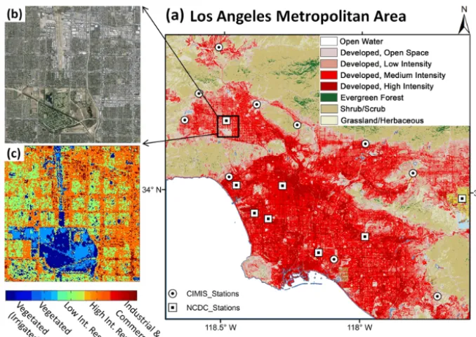
Figure 1. (a) NOAA C-CAP land cover map of the Los Angeles metropolitan area including study domain, 10 CIMIS stations (white circles), and 8 NCDC stations (white squares); (b) Google image of the study domain; and (c) the Noah-UCM urban land cover classification of the study domain.
2 Study area
The study domain is a 49 km2 highly developed neighbor-hood in the city of Los Angeles (Fig. 1). Los Angeles is the second most populous city in the United States with a pop-ulation of 3.8 million (US Census, 2011), covering an area of 1215 km2in southern California. The city has a Mediter-ranean climate and receives 381 mm of annual precipita-tion, mostly over the winter months (NOAA-CSC, 2003; SCDWR, 2009). Due to the semiarid nature of the region, the city’s water supply is heavily dependent on imported wa-ter (52 % from the Colorado River and 36 % from the Los Angeles Aqueduct (Los Angeles Department of Water and Power (LADWP), 2010). Regional water demands and the extensive dependence on external sources make accurate spa-tial representation of the metropolitan area in regional land surface/atmospheric models imperative for predicting current and future water budgets. The study domain includes com-mercial/industrial as well as low- and high-intensity residen-tial land cover types and a large park with both irrigated and nonirrigated landscapes (Fig. 1b and c).
3 Remotely sensed parameters
Remote sensing data are retrieved from Landsat ETM+ im-ages with a nominal pixel resolution of 30 m in the shortwave bands and 60 m in the thermal band. The level 1 Gt ETM+
imagery from USGS EROS, spanning years 2010–2011, are calibrated and atmospherically corrected through the
Landsat Ecosystem Disturbance Adaptive Processing System (LEDAPS). Study domain data are not affected by the failure of the Landsat-7 ETM+Scan Line Corrector in 2003 (SLC-off). Using a knowledge-based approach, similar to the one introduced by Song and Civco (2002), several binary masks are applied to the images to detect contaminated areas (cloud and shadow). Images with cloud and/or shadow are distin-guished and omitted in the following parameter retrievals. A total of 24 pure images, acquired over 2 years, are utilized in the parameter estimation processes.
In addition to Landsat observations, MODIS products from Terra and Aqua satellite platforms are also utilized. The MODIS MCD43A BRDF (bidirectional reflectance distribu-tion funcdistribu-tion) products, concurrent with pure Landsat im-ages, are collected for use in the parameter calculations. The 500 m BRDF products are generated by the MODIS Adap-tive Processing System (MODAPS) at the Goddard Space Flight Center (GSFC), using a kernel-driven linear model, and distributed through the Land Processes DAAC (Dis-tributed Active Archive Center; Justice et al., 2002; Schaaf et al., 2002; Shuai et al., 2008). The described Landsat and MODIS-based data are used to produce a group of six re-motely sensed derivatives, as follows.
Green vegetation fraction (GVF)
[image:3.612.129.468.65.305.2]reflectance values from the red (ρETM3) and near-infrared (ρETM4) bands of Landsat ETM+are used to derive NDVI maps for each date of imagery based on Eq. (1). Next, assum-ing the vegetated part of a pixel is covered by dense vegeta-tion (i.e., it has a high LAI), GVF is calculated using Eq. (2).
NDVI=ρETM4−ρETM3
ρETM4+ρETM3
, (1)
GVF= NDVI−NDVIo
NDVI∞−NDVIo
, (2)
where NDVIoand NDVI∞are constant values computed us-ing signals from bare soil and densely vegetated pixels in the study domain, respectively.
Impervious surface area (ISA)
ISA is shown to be inversely proportional to vegetation frac-tion where non-vegetated pervious surfaces are rare (Bauer et al., 2007). Since the majority of pervious surfaces in the studied domain are vegetated and heavily irrigated through-out the year, ISA is assumed to be the complement of the vegetation fraction:
ISA=(1−GVFmax)·100, (3)
where GVFmax is the maximum GVF detected over the 2-year study period. The produced ISA map shows high ac-curacy (> 95 %) when compared to a previously developed high-resolution land cover map, based on QuickBird remote sensing data, aerial photographs, and geographic informa-tion systems over the city of Los Angeles (McPherson et al., 2008). We speculate that one cause that may contribute to the high accuracy of this assumption is that ISA overestima-tion, induced by non-vegetated pervious surfaces, is offset by tree canopies that cover areas larger than underlying pervious surfaces.
Albedo
With a recent methodology by Shuai et al. (2011) em-ployed, 30 m land surface albedo maps are generated uti-lizing Landsat surface reflectance and anisotropy informa-tion from concurrent 500 m MODIS BRDF products. Land-sat data are reprojected from UTM to MODIS sinusoidal pro-jection and aggregated from 30 to 500 m. Using USGS-based land cover types, the percentage of each land cover class within each MODIS pixel is computed, then relatively pure pixels (> 85 % purity) are selected for each class. MCD43A2 quality assessment product is used to choose highest-quality MODIS MCD43A1 BRDF parameters for the pure pix-els. The concurrent parameters are used to calculate nadir reflectance, white-sky albedo, and black-sky albedo under the solar geometry at Landsat overpass time and MODIS
scale. Next, the spectral albedo-to-nadir reflectance ratios, for white-sky and black-sky albedos, are calculated over the pure pixels. The resultant ratios, specific to each land cover class, are applied to Landsat surface reflectance to gener-ate the spectral white-sky and black-sky albedos for each Landsat pixel. A further narrowband-to-broadband conver-sion based on extensive radiative transfer simulations by Liang (2000) is applied to generate the broadband albedos in a shortwave regime. Finally, albedo (blue sky) is modeled as an interpolation between the black-sky (αbs) and white-sky (αws) albedos as a function of the fraction of diffuse sky-light (S(θ,τ (λ)) which is estimated by the 6S (Second Simu-lation of the Satellite Signal in the Solar Spectrum) codebase (Eq. 4; Schaaf et al., 2002).
∝(θ, λ)= {1−S(θ, τ (λ))}αbs(θ, λ)+S (θ, τ (λ)) αws(θ λ), (4) whereτ,θ, andλare optical depth, solar zenith, and wave-length, respectively.
Leaf area index (LAI)
Stenberg et al. (2004) showed that a reduced simple ratio (RSR) explains 63–75 % of the variations in LAI and that maps of projected LAI, based on RSR, have good agreement with observations. In the current study, LAI values are re-trieved based on the LAI–RSR correlations, which are spec-ified utilizing table-based LAI estimates in pure (fully vege-tated) pixels and remotely sensed RSR maps. The atmospher-ically corrected reflectance values of Landsat ETM spec-tral channels red (ρETM3), near infrared (ρETM4), and mid-infrared (ρETM5), implemented in the following Eq. (5), de-fine RSR:
RSR=ρETM4
ρETM3
ρ5max−ρETM5
ρ5max+ρ5min
, (5)
whereρETM5min andρETM5max are the smallest and largest mid-infrared reflectance detected in the Landsat ETM images over the study domain, excluding open water pixels. Emissivity
mixture of man-made material and vegetation (NDVI > 0.2 and ≤0.5), and (4) water bodies (NDVI < 0). Mean emis-sivity values of 0.980, 0.920, and 0.995 are then used for fully vegetated, built-up, and water pixels (Similar to Tan and Li, 2013). Emissivity values (ε) for mixed pixels (class 3) are estimated using the following equations (for details see Stathopoulou et al., 2007):
ε=0.017PV +0.963, (6)
PV =
(NDVI−0.2)2
(0.5−0.2)2 . (7)
Land surface temperature (LST)
The emissivity-corrected land surface temperature (LST) is calculated as follows (Artis and Carnahan, 1982):
LST= BT
n
1+hλ·BT
ρ ·lnε
io, (8)
where BT is Landsat at sensor brightness temperature (K),λ andεare the wavelength of emitted radiance (11.5 µm) and surface emissivity, andρ=hc/σ(1.438×10−2m K), where σ, h, and c are Boltzmann constant, Planck’s constant, and the velocity of light, respectively.
4 Numerical modeling system 4.1 Noah LSM–UCM model
Land surface processes are parameterized using the offline Noah LSM (Chen and Dudhia, 2001) coupled with the single-layer UCM (Kusaka et al. 2001; Kusaka and Kimura, 2004). The Noah LSM is based on a diurnally dependant Penman potential evaporation approach, a multilayer soil pa-rameterization, a canopy resistance model, surface hydrol-ogy, and frozen ground physics (Chen et al., 1996, 1997; Chen and Dudhia, 2001; Ek et al., 2003). The UCM parame-terization includes urban building geometry, shadowing from buildings, reflections and trapping of radiation in a street canyon, and an exponential wind profile. The Noah LSM pro-vides surface sensible and latent heat fluxes and surface skin temperature for vegetated areas (e.g., parks and trees), and the UCM calculates the fluxes for impervious surfaces. The outputs from the Noah LSM and UCM are coupled through the urban surface fractions.
4.2 Irrigation module
Irrigation is accounted for in the Noah-UCM modeling framework by incorporating an urban irrigation module de-veloped in our previous work (Vahmani and Hogue, 2013, 2014). The developed irrigation scheme mimics the effects of urban irrigation by increasing soil moisture content in vege-tated portion of grid pixels at a selected interval. Added an-thropogenic soil moisture contribution is a function of the
soil moisture deficit, which is the difference between irri-gated soil moisture content and actual soil moisture con-tent in the top soil layer. The irrigation module calcu-lates irrigated soil moisture content (SMCIRR; m3m−3), soil moisture deficit (DEF; m3m−3), and irrigation water (IRR; kg m−2s−1) as
SMCIRR=αSMCmax, (9)
DEF=max{[SMCIRR−SMC1],0}, (10) IRR=ρw
1tDEFD1, (11)
where the saturation soil moisture content (SMCmax; m3m−3) and irrigation demand factor (α; unitless) define irrigated soil moisture content (Eq. 9); and D1 is top soil layer thickness (10 cm);ρw (kg m−3) and 1t stand for water density and Noah-UCM time step (3600 s), respectively. The parameter α, ranging from zero to one, regulates the amount of irrigation water added to the soil each time the scheme increases the soil moisture, simulating an irrigation event. Similar to previous studies (Hanasaki et al. 2008a, b; Pokhrel et al. 2012) an irrigation demand factor of 0.75 is utilized in the current work. The irrigation interval is set to three times per week according to the water restrictions implemented by LADWP in 2010.
4.3 Improving the UCM-simulated LST
The calculation of the impervious surface temperature in the UCM version used in this study has been shown to be inaccu-rate (Li and Bou-Zeid, 2014). This is due to the fact that the turbulent transfer coefficient (Ch) for the whole pixel is cal-culated using only momentum and thermal roughness lengths of vegetated portion, ignoring the developed surface impact onCh. Li and Bou-Zeid (2014) showed that this inconsis-tency could result in large biases in simulated LST values. In the current study, an alternative LST calculation, proposed by Li and Bou-Zeid (2014), is used as follows. First, a re-vised surface temperature of the impervious part of the pixel (Ts) is calculated based on canyon temperature (Tc) and roof surface temperature (Tr):
Ts=fr×Tr+(1−fr)×Tc, (12) wherefris the roof fraction of the impervious surface. Note that theTc calculated by the UCM is an equivalent aerody-namic surface temperature aggregated for canyon surfaces, including walls and roads. Next, the LST for the whole grid cell is computed as a weighted average based on theTs and surface temperature of pervious part (T1):
LST=furb×Ts+(1−furb)×T1, (13) wherefurbis the urban fraction of the pixel.
4.4 Land cover data and forcing fields
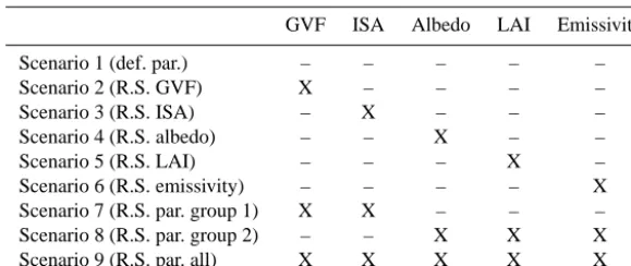
Table 1. Model scenarios (1–9) and the incorporated remotely sensed parameter sets.
GVF ISA Albedo LAI Emissivity
Scenario 1 (def. par.) – – – – –
Scenario 2 (R.S. GVF) X – – – –
Scenario 3 (R.S. ISA) – X – – –
Scenario 4 (R.S. albedo) – – X – –
Scenario 5 (R.S. LAI) – – – X –
Scenario 6 (R.S. emissivity) – – – – X
Scenario 7 (R.S. par. group 1) X X – – –
Scenario 8 (R.S. par. group 2) – – X X X
Scenario 9 (R.S. par. all) X X X X X
type, slope type, vegetation type, and urban type. A com-bination of the Soil Data Mart (http://sdmdataaccess.nrcs. usda.gov/) and the Los Angeles Department of Public Works (LADPW) databases are used to gather soil classification in-formation. Land use and land cover are parameterized us-ing the 30 m NOAA C-CAP-2006 land cover data which is transformed to urban and vegetation type spatial maps over the study domain. High-, medium-, and low-intensity de-veloped land cover types, recognized by NOAA, are con-verted to UCM industrial/commercial, high-intensity, and low-intensity residential types, respectively. The developed open space, along with natural land types, is categorized as 1 of the 27 Noah LSM vegetation classes.
The offline Noah LSM–UCM is forced utilizing hourly ground-based observations from CIMIS and National Cli-matic Data Center (NCDC) stations for the period from 1 January 2010 to 31 December 2011. There are 10 CIMIS and 8 NCDC stations within close proximity of the study do-main (Fig. 1a). The NCDC stations, which use Automated Surface Observing Systems (ASOS), are located at smaller local airports (six stations), one major airport (Los Ange-les International Airport), and a university campus (Univer-sity of Southern California, USC) within the Los Angeles metropolitan area. Reporting the meteorological conditions, the NCDC stations are used for wind speed, air tempera-ture, relative humidity, air pressure, and incoming longwave radiation. All NCDC data are gathered at a standard refer-ence height of 2 m. The regional CIMIS stations are utilized for solar radiation (using LI200S pyranometer) and tipping bucket rain gauges in 18 stations (NCDC and CIMIS) are included in collection of precipitation data. Inverse-distance weighting (second power) is employed to create the spatially gridded forcing fields. Linear interpolation and data from the nearest gage are utilized to replace missing data.
5 Numerical experiments and evaluation methods
5.1 Remote-sensing-based parameterization
5.2 Model evaluation approach
In order to evaluate the performance of the Noah-UCM mod-eling framework, simulated LSTs are compared with con-current Landsat observations and simulated latent heat flux time series are assessed against CIMIS-based ET observa-tions. The CIMIS network was established in 1982 by the CDWR (California Department of Water Resources) and the University of California at Davis in order to provide real-time weather conditions and irrigation water need estimates for California’s agricultural community. The automated CIMIS stations measure hourly surface solar radiation, temperature, humidity, wind, precipitation, soil temperature, and surface pressure (http://wwwcimis.water.ca.gov). The reference ET (ET0) is calculated for each site, utilizing observed meteo-rological fields over a well-watered soil. Utilizing a method-ology introduced by CDWR (2000), actual urban landscape ET is estimated using ET0and a landscape coefficient, which is a function of species, density, and microclimate factors. Based on the authors’ knowledge in the study landscape as well as a report by CDWR (2000), we assume “moderate” (trees and shrubs) and “high” (turf grass) water needs. Fol-lowing the CDWR (2000) instructions on irrigation zones with mixed water need categories (i.e., low, moderate, and high), a value from the high category is selected (average species factor=0.80). Assuming the “average” category for vegetation density, a density factor of 1 is used. Further-more, a “high” category of microclimate condition is used (microclimate factor=1.25) for the current highly devel-oped study domain. This factor is utilized to take into ac-count the contribution of the developed surfaces to the wa-ter loss from vegetated areas, through anthropogenic heat-ing, reflected light, and high temperatures of surrounding heat-absorbing surfaces (e.g., paving and buildings). Using these factors, a landscape coefficient of 1 (landscape coef-ficient=species factor×density factor×microclimate fac-tor) is prescribed. This coefficient and ET0estimations from 10 CIMIS stations within close proximity of the study do-main (Fig. 1a) are utilized to compute the urban landscape ET. Inverse-distance weighting (second power) is employed to create spatially gridded ET maps over fully vegetated pix-els in the study area which are then used in validation pro-cesses of the Noah UCM. ET output of the model is also evaluated against recent ET measurements in the greater Los Angeles area (Moering, 2011). Moering (2011) employed a previously developed chamber approach to measure instan-taneous ET in an irrigated and a nonirrigated park in the Los Angeles metropolitan area during WY (water year) 2011 (WY is defined as 1 October of the previous year to 30 September of the designated year). They reported an annual ET of about 1224 mm over the observed irrigated park, which is located within our study domain.
6 Sensitivity study of surface parameter 6.1 Temporal evaluation
The monthly time series of the default Noah UCM and remote-sensing-based GVF, ISA, albedo, and LAI are com-pared and modeled cumulative monthly sensible and latent heat fluxes, using default and newly estimated parameters, are presented over fully vegetated, low-intensity residential, and industrial/commercial areas (Fig. 2). Fluxes from high-intensity residential areas are not presented as they behave similarly to those from the industrial/commercial areas. Ex-cept for the summer months, GVF values are significantly increased throughout the year when remote sensing prod-ucts are utilized (Fig. 2a). Moreover, the default seasonal variations of GVF values, assumed over all the land cover types, are not detected in Landsat imagery (Fig. 2a). The reason for this is the significant and year-round irrigation in the Los Angeles area, which is not accounted for in the de-fault parameter tables. This is confirmed by previous stud-ies (Johnson and Belitz, 2012) that reported urban vegeta-tion supported by water delivery, in contrast to common sea-sonal behavior of greening in the winter/spring and brown-ing in the summer, maintains constant greenness, which is reflected in NDVI and GVF estimates. GVF plays a dom-inant role in the Noah-UCM simulations as it defines the vegetated fraction of the natural areas, and specifies albedo, LAI, emissivity, and roughness length values from the prede-fined ranges in the model lookup tables. Furthermore, GVF partitions the total ET between soil direct and canopy ET. The simulated latent heat flux is considerably decreased (up to 139 MJ m−2month−1) in the summertime and increased over the remaining months, when remotely sensed GVF is incorporated in the fully vegetated areas (Fig. 2b). Since any increase of latent heat flux that does not alter the radiative balance leads to a reduction in sensible flux, the newly de-veloped GVF values, in turn, cause enhancements (up to 103 MJ m−2month−1) in the simulated summer sensible heat fluxes and a reduction in the sensible heat fluxes during the remaining months (Fig. 2b). Latent and sensible heat fluxes from the low-intensity residential pixels show similar but less significant changes (up to 66.1 and 31.0 MJ m−2month−1, respectively) when the new parameter sets are implemented. Adding remotely sensed GVF causes insignificant changes in the industrial/commercial area fluxes due to the small per-centage of vegetated land cover in such areas (Fig. 2d).
Figure 2. Monthly time series of default Noah UCM compared with remote-sensing-based GVF, ISA, albedo, and LAI (row 1), as well as modeled cumulative monthly sensible and latent heat fluxes (MJ m−2) over fully vegetated (row 2), low-intensity residential (row 3), and industrial/commercial areas (row 4) using the default and newly estimated parameters: (b–d) GVF, (f–h) ISA, (j–l) albedo, and (n–p) LAI.
of urban fraction in partitioning of the energy fluxes. Over the low-intensity residential areas, higher ISA values min-imize the effects of urban vegetation, which leads to la-tent heat fluxes decreases (up to 62.6 MJ m−2month−1) and sensible heat fluxes increases (up to 52.4 MJ m−2month−1), throughout the year, when remotely sensed data replace de-fault urban fractions (Fig. 2g). These changes are reversed and less significant over the industrial and commercial pixels (maximum latent and sensible heat flux changes of 30.0 and 26.5 MJ m−2month−1, respectively; Fig. 2h). ISA has no in-fluence on the fluxes from fully vegetated pixels which do not include impervious areas (Fig. 2f).
Considerable changes in the monthly albedo averages are detected when incorporating remote sensing data in the pa-rameterization process (Fig. 2i). With the use of fused Land-sat and MODIS products, a reduction of averaged albedo values is observed over the fully vegetated and residen-tial areas (up to 48 and 39 %, respectively; Fig. 2i). More-over, the default seasonal variations are hardly noticeable in the remote-sensing-based albedo values, which is due to the consistent greenness in the study area from irriga-tion throughout the year. On the other hand, considerable albedo increases (up to 39 %) are detectable over the in-dustrial/commercial pixels (Fig. 2i), which are caused by bright and highly reflective materials seen mainly over the rooftops of industrial/commercial buildings. Albedo affects
the radiative energy budget and consequently available en-ergy for the turbulent fluxes. In the current study, de-creased albedo values over the fully vegetated and low-intensity residential areas result in reduced loss of solar and longwave radiation, respectively, and, in turn, increases the sensible heat flux (up to 33.8 and 21.5 MJ m−2month−1; Fig. 2j and k). Albedo-induced sensible heat deceases over industrial/commercial pixels are also noticeable (up to 33.9 MJ m−2month−1; Fig. 2l).
of the canopy resistance, controlling canopy ET rates. In the presented results (Fig. 2n and o), LAI-induced changes in the simulated turbulent fluxes are more apparent in the summer months and over fully vegetated and residential pixels, where sensible heat flux is significantly increased (up to 57.2 and 86.5 MJ m−2month−1, respectively) and la-tent heat flux is significantly decreased (up to 65.5 and 97.9 MJ m−2month−1, respectively). This is due to the con-siderable deceases in the LAI values in summertime which lead to elevations of the canopy resistance and therefore re-ductions of the transpiration from the vegetation, causing de-creases in latent heat fluxes. This in turn partitions the net radiation more into sensible heat fluxes. LAI does not affect fluxes from industrial/commercial pixels with small pervious fractions (Fig. 2p). It is worth mentioning that changes in the turbulent fluxes time series, in particular the latent heat flux decreases in the summer months induced by implemen-tation of satellite-based LAI, are to some extent captured in the simulations with the remote-sensing-based GVF (com-pare Fig. 2b with n and c with o). This reflects our previ-ous point that GVF controls assigned LAI values to vege-tated pixels in the Noah LSM and that realistic presentation of GVF in the modeling framework can enhance LAI inputs in the model when LAI measurements are not available.
Remotely sensed emissivity maps are also utilized to replace the default values in the Noah-UCM simulations, which results in changes in the emissivity values (up to 5.1 %). However, the new surface parameterization leads to insignificant changes in turbulent fluxes (results now shown). The largest emissivity induced alterations in sen-sible heat fluxes are seen over industrial and commercial pixels (up to 31.2 MJ m−2month−1). Latent heat fluxes are changed most significantly over fully vegetated areas (up to 2.56 MJ m−2month−1).
6.2 Spatial evaluation
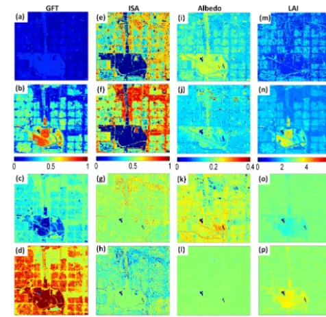
The spatial distributions of newly assigned GVF, ISA, albedo, and LAI are next compared with those based on the Noah-UCM lookup tables. Different urban surface parame-terizations, along with their impacts on the simulated maps of turbulent sensible and latent heat fluxes, are presented (Fig. 3; valid at 11:00 LST on 14 April 2011). As expected, during the spring period (April), GVF values are significantly higher when remote sensing products are utilized, due to the irrigation effects which are ignored in the default parameters (Fig. 3a and b). Over fully vegetated and low-intensity resi-dential pixels, where a significant portion of the energy goes into evaporation and transpiration, latent heat flux increases (about 300 and 230 W m−2, respectively) and sensible heat fluxes decreases (about 160 and 120 W m−2, respectively) are found (Fig. 3c and d) when utilizing the remote sensing GVF.
[image:9.612.310.548.65.296.2]The spatial distributions of ISA, or urban fraction, between the remote sensing and default values show similar patterns
Figure 3. Spatial distributions of GVF, ISA, albedo, and LAI based on Noah-UCM lookup tables (row 1) compared with remotely sensed values (row 2) and simulated difference maps of sensi-ble (row 3) and latent (row 4) heat fluxes using default and re-motely sensed urban surface parameters: (c and d) GVF, (g and h) ISA, (k and l) albedo, and (o and p) LAI. Valid at 11:00 LST on 14 April 2011.
(Fig. 3e and f). However, industrial/commercial and high-intensity residential areas are assigned noticeably higher ur-ban fraction values in the remote-sensing-based maps (com-pare Fig. 3e with f), which leads to lower latent heat fluxes (bias of up to about 130 W m−2) and higher sensible (bias of up to about 100 W m−2) in these pixels (Fig. 3g and h).
The Noah-UCM parameters, based on lookup tables, un-derestimate surface albedo values over highly urbanized pix-els when compared with remote sensing data (Fig. 3i and j). In particular, the industrial/commercial buildings with highly reflective rooftops are completely ignored. Over the highly vegetated areas, however, albedo values are slightly over-estimated in lookup tables. With the energy budget altered, the newly developed albedo data sets lead to lower Noah-UCM-simulated sensible heat fluxes over intensely devel-oped pixels (Fig. 3k). The sensible heat flux differences are only significant over industrial/commercial pixels, which in-clude buildings with bright roofs (up to∼300 W m−2). The changes in absolute surface albedos do not affect simulated latent heat fluxes as these reflective roofs are located in in-dustrial/commercial areas with negligible pervious surfaces and simulated latent heat flux (Fig. 3l).
the spatial distribution of turbulent fluxes (Fig. 3o and p). Over the densely vegetated areas, increases in latent heat flux (up to 50 W m−2) and decreases in sensible heat flux (up to 35 W m−2) are found (Fig. 3o and p). It is noteworthy that, as illustrated before (Fig. 3n and o), the most significant influ-ences of LAI alterations are detected in the summer months. Thus, it is not surprising that the turbulent fluxes do not show significant sensitivity to the LAI changes in April.
Remotely sensed emissivity maps, implemented in the Noah-UCM simulations, show minimal effect on the output turbulent fluxes maps (results not shown). Our results (Figs. 2 and 3) agree with previous sensitivity studies performed with the Noah UCM, which indicated high sensitivity of the model to GVF, ISA, albedo, and LAI, and less model sensitivity to emissivity (Loridan et al., 2010; Wang et al., 2011). Loridan et al. (2010) highlighted the critical role of ISA and LAI in the simulations of latent heat flux and albedo role in the sen-sible heat flux simulations. Investigating the peaks of diurnal turbulent fluxes, Wang et al. (2011) reported that latent heat flux is the most sensitive to the GVF. They also found that emissivity has minimal effects on the model outputs.
7 Evaluation of Noah-UCM performance
After initial sensitivity tests, the model performance in repro-ducing ET and LST fields is evaluated using remotely sensed (independent from derived parameters) and in situ measure-ments. The comparisons of observed and simulated ET and LST, using different urban surface parameterizations (scenar-ios 1, 7, 8, and 9 in Table 1), are presented in Figs. 4, 5, and 6. 7.1 ET simulations
[image:10.612.309.545.68.379.2]The temporal variations of ET, simulated by the Noah-UCM model and averaged over fully vegetated pixels, are evaluated against CIMIS-based ET measurements, spanning 2010 and 2011 (Fig. 4). The presented observations are averages over fully vegetated pixels in the study domain, calculated using ET maps based on ET0measurements from 10 CIMIS sta-tions, landscape coefficients, and inverse-distance weighting (second power; see Sect. 5.2). The model reproduces simi-lar ET behaviors when the default parameters and the second group of remotely sensed parameters (albedo, LAI, and emis-sivity) are implemented (Fig. 4a and c). The ET differences between observations and the default simulation are minimal in the winter and fall months, due to the limited energy avail-able for ET in those months. Over the warmer months, the observed and modeled ETs show distinct behaviors. CIMIS stations report two peaks: one in the spring and one in the summertime. Simulated ETs, however, illustrate one peak in July. The Noah UCM, using these parameterizations, under-estimates ET rates for the most of winter and spring months and overestimates them in the summertime (Fig. 4a and c). Including remotely sensed albedo, LAI, and emissivity does
Figure 4. Noah-UCM-simulated cumulative monthly ET, averaged over fully vegetated pixels using different urban surface parameter-izations: scenarios (a) 1, (b) 7, (c) 8, and (d) 9 in the Table 1 and their comparisons with CIMIS-based ET measurements spanning 2010 and 2011. Scatter plots of these comparisons are also included (right).
not change the general seasonal pattern deviations of ET (Fig. 4a and c), but it reduces the biases considerably (with R2=0.83 and RMSE=14.32 mm month−1). We note that model improvement is mostly associated with inclusion of remotely sensed LAI maps in the model since albedo and emissivity have minimal influence on latent heat fluxes from heavily vegetated pixels (see Fig. 2j).
changes enhance the model performance significantly (with R2=0.92 and RMSE=11.77 mm month−1).
Including all the measured parameter sets (Fig. 4d) re-duces the behavioral disagreements between observed and modeled monthly ET (R2=0.86). Large biases over the summer months are also reduced. However, ET values are overestimated over the rest of the year (RMSE=
17.49 mm month−1). Although each newly developed pa-rameter group enhances the model performance in predicting ET, the advantages are countered when all of the parameters are implemented in the model. This is possibly due to the complex interactions between the parameters (e.g., GVF and LAI) in the model structure.
A notable pattern detected by CIMIS data is the drop in ET values over the month of June. The sudden decrease in ET corresponds to the “June gloom” weather pattern in south-ern California, when onshore flows result in persistent over-cast skies with cool temperatures, as well as fog and driz-zle in late spring and early summer (NWS, 2011). The June gloom effects are captured in scenarios 7 and 9 (Fig. 4b and d) and not seen in scenarios 1 and 8 (Fig. 4a and c). Since ISA has minimal influence on ET from the fully vegetated pixels and the second group fails to simulate June gloom influence, the improvements in scenarios 7 and 9 in capturing this phe-nomenon are associated with a more accurate representation of GVF.
7.2 LST simulations
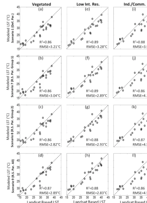
In order to further evaluate model performance and exam-ine the impacts of different remote-sensing-based parameter sets, Landsat-based LST measurements are utilized (Figs. 5 and 6). Statistics (R2and RMSE) are also included to quan-tify the model performance using different urban surface pa-rameterizations (Fig. 5). The observed LSTs over fully veg-etated pixels are estimated with fair accuracy by the default model (R2=0.86 and RMSE=3.21◦C; Fig. 5a). The model performance has almost the same level of accuracy over low-intensity residential areas and is slightly worse (< 1◦C) over industrial/commercial pixels (Fig. 5e). Using remote sensing data over fully vegetated and low-intensity residential pix-els weakly improves the biases (with < 1◦C improvement; Fig. 5b–d and f–h). Over industrial/commercial areas, a sys-tematic underestimation of the observed LST is identified (RMSE=3.96−4.59◦C; Fig. 5i–l) which seems to be per-sistent after using different remotely sensed parameter sets. We speculate that this underestimation of LST over highly developed areas is due to lack of representation of anthro-pogenic heating in the current study.
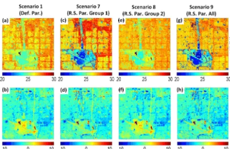
[image:11.612.309.545.66.391.2]A comparison of LST at 11:00 LST on 14 April 2011 with four simulation cases is also presented (Fig. 6). Alterations due to use of remote sensing products are more noticeable in this spatial examination of the results. Using all the default parameters (scenario 1), observed LST is overestimated over
Figure 5. Scatter plots of observed (Landsat-based) versus simu-lated LSTs averaged over different land cover types using different urban surface parameterizations, including scenarios 1 (row 1), 7 (row 2), 8 (row 3), and 9 (row 4) in Table 1.
the heavily vegetated areas and underestimated over highly developed pixels (Fig. 6a and b).
Figure 6. Noah-UCM-simulated LST maps using different urban surface parameterizations: scenarios 1, 7, 8, and 9 from Table 1 (top row) as well as differences between simulated and observed land surface temperature at 1100 LST on 14 April 2011 (bottom row).
scenario 7, considerable GVF-induced LST reductions over fully vegetated areas improve the observed LST estimations in scenario 9 (Fig. 6h). Our assessment indicates that imple-mented satellite-derived parameter maps, particularly GVF and ISA used in scenarios 7 and 9, enhance the Noah-UCM capability to reproduce the LST differences between fully vegetated pixels and highly developed areas (simulated LST differences of 3.07, 6.78, 3.48, and 7.30◦C for scenarios 1, 7, 8, and 9 vs. observed LST difference of 11.25◦C). 7.3 Energy and water budget evaluation
Differences in the simulated energy and water budgets, with different surface parameterizations (scenarios 1, 7, 8, and 9 in the Table 1) are summarized for WY 2011 (Fig. 7). The emissivity induced changes to the energy and water budgets are insignificant and not included. The illustrated radiative and turbulent heat fluxes show that, unlike the longwave ra-diative fluxes, the simulated available solar radiations are al-tered considerably using different urban parameter sets (up to 6 %), particularly over fully vegetated (Fig. 7a) and indus-trial/commercial pixels (Fig. 7c). These changes are induced by new surface albedo values utilized in scenarios 8 and 9. It is also observed that most of the incoming radiative energy is dissipated through latent heat fluxes, over heavily vegetated pixels (Fig. 7a and b), and sensible heat fluxes over indus-trial/commercial areas (Fig. 7c). These turbulent fluxes are also altered when different surface parameterizations are in-corporated. Implementing all the remotely sensed parameters (scenario 9), the annual latent heat flux is increased (12 %) over fully vegetated pixels (Fig. 7a), and the annual sensible heat flux is decreased (32 %) over industrial/commercial pix-els (Fig. 7c). Ground heat fluxes, however, are insignificant and unchanged.
Water budget terms also show variable behavior using different parameter sets over different land cover types
Figure 7. Differences in simulated energy (top) and water (bottom) budgets for WY 2011, using different urban surface parameteri-zation and averaged over different land cover types. Energy bud-get terms include shortwave radiation (SW) and longwave radia-tion (LW), as well as sensible (SH), latent (LH), and ground (GH) heat fluxes. Water budget terms include precipitation (PPT), irri-gation water (IRR), evapotranspiration (ET), surface runoff (SFC R.O.), and subsurface runoff (S. SFC R.O.).
(Fig. 7d–f). Annual irrigation amounts exceed received pre-cipitations over the pixels with significant vegetation frac-tions (Fig. 7d and e). This pattern is not rare in semiarid re-gions (CDWR, 1975; Mini et al., 2014). In these areas, most of incoming water is lost through ET (Fig. 7d and e). Areas with high coverage of impervious surfaces, however, dissi-pate most of the incoming moisture through surface runoff (Fig. 7f). The alterations in the annual ET rates are, for the most part, due to the changes in the GVF parameterizations (scenarios 7 and 9; Fig. 7d–f). Sub-surface runoff annual rates, on the other hand, are altered using new ISA values (scenarios 7 and 9; Fig. 7e and f). Changes in the annual ET values are as large as 145, 156, and 79.4 mm over fully veg-etated, low-intensity residential, and industrial/commercial pixels, respectively (Fig. 7d–f).
[image:12.612.310.548.66.216.2]LAI values utilized in scenarios 8 and 9; and (3) complex interactions between GVF and LAI noted in scenario 9.
The presented analysis of energy balance (Fig. 7) suggests that GVF, albedo, and LAI play an important role in regulat-ing simulated radiative energy budget and turbulent fluxes, mainly by affecting the available net radiation and transpira-tion quantities. GVF, ISA, and LAI also alter the study area transpiration and ET values, as well as surface runoff rates.
8 Conclusions
In the current work we investigate the utility of a select set of remote-sensing-based surface parameters in the Noah-UCM modeling framework over a highly developed urban area. It was found that remote sensing data show significantly dif-ferent magnitudes and seasonal patterns of GVF when com-pared with the default values. The reason for this mismatch is the significant and year-round irrigation in the Los Angeles area which is not accounted for in the default parameter ta-bles. Irrigated landscapes maintain constant greenness rather than a seasonal behavior of greening in the winter/spring and browning in the summer. The noticed differences be-tween the monthly LAI values from default tables and re-motely sensed data are also due to complex irrigation pat-terns. Another factor that contributes to this mismatch is the fact that landscape plantings are quite different from agri-cultural crops due to their being composed of collections of vegetation species, which is not taken into account in the veg-etation parameter tables in the Noah LSM (CDWR, 2000; Vahmani and Hogue, 2013, 2014). There are also consider-able deviations between the lookup-tconsider-able-based ISA, albedo and emissivity maps, and the remotely sensed values. The re-sults of our analysis agree with previous studies which show high sensitivity of the Noah UCM to GVF, ISA, albedo, and LAI, and minimal model sensitivity to emissivity (Loridan et al., 2010; Wang et al., 2011). Our results show that GVF, ISA, and LAI are critical in the simulations of latent and sen-sible heat flux, and that albedo plays a key role in the sensen-sible heat flux simulations.
Our assessment of the Noah-UCM ET estimation shows that using the default parameters leads to significant errors in the model predictions of monthly ET fields (RMSE=
22.06 mm month−1) over the study domain in Los Ange-les. Results show that accurate representation of GVF is critical to reproduce observed ET patterns over vegetated areas in the urban domains. LAI also plays an important role in ET simulations. However, simulations incorporat-ing the remotely sensed GVF values outperform (RMSE=
11.77 mm month−1) simulations with the new LAI estimates (RMSE=14.32 mm month−1). This could be due to sev-eral reasons. First, there are uncertainties associated with the remote-sensing-based LAI retrieval, including nonlinearity of LAI–vegetation index (RSR) relationships (Latifi and Ga-los, 2010), which do not apply to NDVI-based GVF. Second,
more accurate representation of GVF values in the Noah UCM not only improves the assigned LAI values to the veg-etated pixels in the model but also enhances other parame-ters’ inputs as well (i.e., albedo, emissivity, and roughness length). Further analysis of the model performance indicates that implemented satellite-derived parameter maps, partic-ularly GVF and ISA, enhance the capability of the Noah UCM to reproduce the LST differences between fully veg-etated pixels and highly developed areas (simulated LST dif-ferences of 3.07 and 6.78◦C for scenarios with default and remotely sensed GVF and ISA vs. observed LST difference of 11.25◦C).
Our analysis of energy balance suggests that GVF, albedo, and LAI play an important role in regulating simulated radia-tive energy budget and turbulent fluxes, mainly by affecting the available net radiation and ET quantities. With regard to urban water balance, GVF, ISA, and LAI play a key role in surface hydrologic fluxes, including ET and surface runoff. When compared with in situ observations, Noah UCM shows the capacity to reproduce ET fields with relatively high accu-racy (Bias of 1.47 mm) when GVF maps are updated using remote sensing data.
Acknowledgements. Funding for this research was supported by an NSF Hydrologic Sciences Program CAREER grant (no. EAR0846662), a 2012 NASA Earth and Space Science Fellowship (no. NNX12AN63H), and an NSF Water Sustainability and Climate (WSC) grant (no. EAR12040235).
Edited by: P. Gentine
References
Arnfield, A. J.: Two decades of urban climate research: A review of turbulence, exchanges of energy and water, and the urban heat island, Int. J. Climatol., 23, 1–26, doi:10.1002/joc.859, 2003. Artis, D. A. and Carnahan, W. H.: Survey of emissivity variability in
thermography of urban areas, Remote Sens. Environ., 12, 313– 329, 1982.
Bauer, M. E., Loeffelholz, B., and Wilson, B.: Estimating and map-ping impervious surface area by regression analysis of Landsat imagery, Remote Sensing of Impervious Surfaces, 3–20, Boca Raton, Florida: CRC Press, 2007.
Bornstein, R.: Urban climate models: Nature, limitations, and ap-plications, Meteorol. Atmos. Phys., 38, 185–194, 1987. Burian, S. J., Stetson, S. W., Han, W., Ching, J., and Byun, D.:
High resolution dataset of urban canopy parameters for Hous-ton, Texas, Preprint proceedings, Fifth Symposium on the Urban Environment, Vancouver, BC, Canada, 23–26 August, Am. Me-teorol. Soc.: Boston, MA, 2004.
Burian, S. J., Brown, M., McPherson, T. N., Hartman, J., Han, W., Jeyachandran, I., and Rush, J.: Emerging urban databases for me-teorological and dispersion, Sixth Symposium on the Urban En-vironment, Atlanta, GA, 28 January–2 February, Am. Meteorol. Soc.: Boston, MA, Paper 5.2, 2006.
Burian, S. J., Brown, M. J., and Augustus, N.: Development and assessment of the second generation National Building Statistics database, Seventh Symposium on the Urban Environment, San Diego, CA, 10–13 September, Am. Meteorol. Soc.: Boston, MA, Paper 5.4, 2007.
California Department of Water Resources (CDWR): California’s ground water, Bulletin 118, Department of Water resources, State of California, 1975.
California Department of Water Resources (CDWR): A guide to estimating irrigation water needs of landscape plantings in Cali-fornia: The landscape coefficient method and WUCOLS III, De-partment of Water Resources, State of California, 1–150, 2000. Changnon, S. A. and Huff, F. A.: The urban-related
nocturnal rainfall anomaly at St. Louis, J. Climate Appl. Meteorol., 25, 1985–1995, doi:10.1175/1520-0450(1986)025<1985:TURNRA>2.0.CO;2, 1986.
Changnon, S. A.: Inadvertent weather modification in urban area: Lessons for global climate change, B. Am. Meteorol. Soc., 73, 619–627, doi:10.1175/1520-0477(1992)073<0619:IWMIUA>2.0.CO;2, 1992.
Chen, F. and Dudhia, J.: Coupling an advanced land-surface/hydrology model with the Penn State/NCAR MM5 modeling system. Part I: model implementation and sensitivity, Mon. Weather Rev., 129, 569–585, 2001.
Chen, F., Mitchell, K., Schaake, J., Xue, Y., Pan, H.-L., Ko-ren, V., Duan, Q. Y., Ek, M., and Betts, A.: Modeling of
land-surface evaporation by four schemes and comparison with FIFE observations, J. Geophys. Res., 101, 7251–7268, doi:10.1029/95JD02165, 1996.
Chen, F., Janjic, Z., and Mitchell, K.: Impact of atmospheric sur-face layer parameterization in the new land-sursur-face scheme of the NCEP mesoscale Eta model, Boundary-Lay. Meteorol., 85, 391–421, doi:10.1023/A:1000531001463, 1997.
Chen, F., Kusaka, H., Tewari, M., Bao, J. W., and Harakuchi, H.: Utilizing the coupled WRF/LSM/urban modeling system with detailed urban classification to simulate the urban heat island phenomena over the Greater Houston area, Paper 9.11, Am. Me-teorol. Soc., Fifth Symposium on the Urban Environment, Van-couver, BC, Canada, 2004.
Chen, F., Kusaka, H., Bornstein, R., Ching, J., Grimmond, C. S. B., Grossman-Clarke, S., Loridan, T., Manning, K. W., Martilli, A., Miao, S., Sailor, D., Salamanca, F. P., Taha, H., Tewari, M., Wang, X., Wyszogrodzki, A. A., and Zhang, C.: The integrated WRF/urban modelling system: development, evaluation, and ap-plications to urban environmental problems, Int. J. Climatol., 31, 273–288, doi:10.1002/joc.2158, 2011.
Cheng, F. Y. and Byun, D. W.: Application of High Resolution Land Use and Land Cover Data for Atmospheric Modeling in the Houston-Galveston Metropolitan Area: Part I, Meteoro-logical Simulation Results, Atmos. Environ., 42, 7795–7811, doi:10.1016/j.atmosenv.2008.04.055, 2008.
Cheng, F. Y., Hsu, Y. C., Lin, P. L., and Lin, T. H.: Investigation of the Effects of Different Land Use and Land Cover Patterns on Mesoscale Meteorological Simulations in the Taiwan Area, J. Appl. Meteorol. Climatol., 52, 570–587, doi:10.1175/JAMC-D-12-0109.1, 2013.
Ching, J., Brown, M., McPherson, T., Burian, S., Chen, F., Cionco, R., Hanna, A., Hultgren, T., Sailor, D., Taha, H., and Williams, D.: National Urban Database and Access Por-tal Tool, NUDAPT, B. Am. Meteorol. Soc., 90, 1157–1168, doi:10.1175/2009BAMS2675.1, 2009.
Cotton, W. R. and Pielke, R. A.: Human impacts on weather and climate, Cambridge: Cambridge University Press, 1995. De Ridder, K., Bertrand, C., Casanova, G., and Lefebvre, W.:
Exploring a new method for the retrieval of urban ther-mophysical properties using thermal infrared remote sensing and deterministic modeling, J. Geophys. Res., 117, D17108, doi:10.1029/2011JD017194, 2012.
Ek, M. B., Mitchell, K. E., Lin, Y., Rogers, E., Grunmann, P., Koren, V., Gayno, G., and Tarpley, J. D.: Implementation of Noah land surface model advances in the National Center for Environmental Prediction operational mesoscale Eta model, J. Geophys. Res., 108, 8851, doi:10.1029/2002JD003296, 2003.
Giannaros, T. M., Melas, D., Daglis, I. A., Keramitsoglou, I., and Kourtidis, K.: Numerical study of the urban heat island over Athens (Greece) with the WRF model, Atmos. Environ., 73, 103–111, doi:10.1016/j.atmosenv.2013.02.055, 2013.
Gutman, G. and Ignatov, A.: Derivation of green vegetation frac-tion from NOAA/AVHRR for use in numerical weather predic-tion models, Int. J. Remote Sens., 19, 1533–1543, 1998. Hanasaki, N., Kanae, S., Oki, T., Masuda, K., Motoya, K.,
Hanasaki, N., Kanae, S., Oki, T., Masuda, K., Motoya, K., Shi-rakawa, N., Shen, Y., and Tanaka, K.: An integrated model for the assessment of global water resources – Part 2: Applica-tions and assessments, Hydrol. Earth Syst. Sci., 12, 1027–1037, doi:10.5194/hess-12-1027-2008, 2008b.
Jiang, X., Wiedinmyer, C., Chen, F., Yang, Z. L., and Lo, J. C. F.: Predicted impacts of climate and land use change on sur-face ozone in the Houston, Texas, area, J. Geophys. Res., 113, D20312, doi:10.1029/2008JD009820, 2008.
Jin, M. and Shepherd J. M.: Inclusion of urban landscape in a cli-mate model – How can satellite data help?, B. Am. Meteorol. Soc., 86, 681–689, doi:10.1175/BAMS-86-5-681, 2005. Johnson, T. D. and Belitz K.: A remote sensing approach for
es-timating 1 the location and rate of urban irrigation in semi-arid climates, J. Hydrology, 414–415, 86–98, 2012.
Justice, C. O., Townshend, J. R. G., Vermote, E. F., Masuoka, E., Wolfe, R. E., Saleous, N., Roy, D. P., and Morisette, J. T.: An overview of MODIS land data processing and product status, Re-mote Sens. Environ., 83, 3–15, 2002.
Kalnay, E. and Cai, M.: Impact of urbanization and land-use change on climate, Nature, 423, 528–531, 2003.
Kusaka, H. and Kimura, F.: Thermal effects of urban canyon struc-ture on the nocturnal heat island:Numerical experiment using a mesoscale model coupled with an urban canopy model, J. Appl. Meteorol., 43, 1899–1910, 2004.
Kusaka, H., Kondo, H., Kikegawa, Y., and Kimura, F.: A simple single-layer urban canopy model for atmospheric models: Com-parison with multi-layer and slab models, Boundary-Lay. Mete-orol., 101, 329–358, 2001.
Landsberg, H. E.: The urban climate, New York: Academic Press, 1981.
Latifi, H. and Galos, B.: Remote sensing-supported vegetation pa-rameters for regional climate models: a brief review, iForest, 3, 98–101, doi:10.3832/ifor0543-003, 2010.
Li, D. and Bou-Zeid, E.: Quality and Sensitivity of High-Resolution Numerical Simulation of Urban Heat Islands, Environ. Res. Lett., 9, 055001, doi:10.1088/1748-9326/9/5/055001, 2014.
Liang, S.: Narrowband to broadband conversions of land surface albedo: I Algorithms, Remote Sens. Environ., 76, 213–238, 2000.
Loridan, T., Grimmond, C. S. B., Grossman-Clarke, S., Chen, F., Tewari, M., Manning, K., Martilli, A., Kusaka, H., and Best, M.: Trade-offs and responsiveness of the single-layer urban param-eterization in WRF: an offline evaluation using the MOSCEM optimization algorithm and field observations, Q. J. R. Meteorol. Soc., 136, 997–1019, doi:10.1002/qj.614, 2010.
Lowry, W.: Urban effects on precipitation amount, Prog. Phys. Geog., 22, 477–520, doi:10.1177/030913339802200403, 1998. Marshall, C. H., Pielke, R. A., Steyaert, L., and Willard,
D.: The impact of anthropogenic land-cover change on the Florida peninsula sea breezes and warm season sensible weather, Mon. Weather Rev., 132, 28–52, doi:10.1175/1520-0493(2004)132<0028:TIOALC>2.0.CO;2, 2004.
Martilli, A., Clappier, A., and Rotach, M. W.: An urban surface ex-change parameterization for mesoscale models, Boundary-Lay. Meteorol., 104, 261–304, 2002.
McPherson, E. G., Simpson, J. R., Xiao, Q., and Wu, C.: Los An-geles 1-million tree canopy cover assessment, Gen. Tech. Rep.
PSW-GTR-207, Albany, CA: US Department of Agriculture, Forest Service, Pacific Southwest Research Station, 52 p., 2008. Miao, S. and Chen, F.: Formation of horizontal convec-tive rolls in urban areas, Atmos. Res., 89, 298–304, doi:10.1016/j.atmosres.2008.02.013, 2008.
Miao, S., Chen F., LeMone, M. A., Tewari M., Li, Q., and Wang, Y.: An observational and modeling study of characteristics of urban heat island and boundary layer structures in Beijing, J. Appl. Me-teorol. Climatol., 48, 484–501, doi:10.1175/2008JAMC1909.1, 2009.
Mini, C., Hogue, T. S., and Pincetl, S.: Estimation of Residential Outdoor Water Use in Los Angeles, California, Landscape Urban Plan., 127, 124–135, doi:10.1016/j.landurbplan.2014.04.007, 2014.
Moering, D. C.: A comparative study of evapotranspiration rates between irrigated and non-irrigated parks in Los Angeles, M.S. thesis, Dep. of Civil and Env. Eng., University of California Los Angeles, Los Angeles, California, 2011.
National Oceanographic and Atmospheric Administration-Coastal Services Center (NOAA-CSC): Southern California 2000-Era Land Cover/Land Use, LANDSAT-TM, 10m, NOAA-CSC, Charleston, SC, 2003.
National Weather Service (NWS): Jet Stream – The Marine Layer, NOAA National Weather Service, available at: http://www.srh. noaa.gov/jetstream/ocean/marine.htm (last access: 24 February 2013), 2011.
Niyogi, D., Holt, T., Zhong, S., Pyle, P. C., and Basara, J.: Urban and land surface effects on the 30 July 2003 mesoscale convective system event observed in the Southern Great Plains, J. Geophys. Res., 111, D19107, doi:10.1029/2005JD006746, 2006.
Pielke, R. A. Sr., Marland, G., Betts, R. A., Chase, T. N., Eastman, J. L., Niles, J. O., Niyogi, D., and Running, S.: The influence of land-use change and landscape dynamics on the climate system: Relevance to climate change policy beyond the radiative effect of greenhouse gases, Phil. Trans. R. Soc. London A, 360, 1705– 1719, 2002.
Pokhrel, Y., Hanasaki, N., Koirala, S., Cho, J., Kim, H., Yeh, P. J.-F., Kanae, S., and Oki, T.: Incorporating anthropogenic water regulation modules into a land surface model, J. Hydrometeorol., 13, 255–269, doi:10.1175/JHM-D-11-013.1, 2012.
Schaaf, C. B., Gao, F., Strahler, A. H., Lucht, W., Li, X. W., Tsang, T., Strugnell, N. C., Zhang, X. Y., Jin, Y. F., Muller, J. P., Lewis, P., Barnsley, M., Hobson, P., Disney, M., Roberts, G., Dun-derdale, M., Doll, C., d’Entremont, R. P., Hu, B. X., Liang, S. L., Privette, J. L., and Roy, D.: First operational BRDF, albedo nadir reflectance products from MODIS, Remote Sens. Environ., 83, 135–148, 2002.
Shuai, Y., Schaaf, C. B., Strahler, A. H., Liu, J., and Jiao, Z.: Quality assessment of BRDF/albedo retrievals in MODIS operational system, Geophys. Res. Lett., 35, L05407, doi:10.1029/2007GL032568, 2008.
Shuai, Y., Masek, J. G., Gao, F., and Schaaf, C. B.: An algorithm for the retrieval of 30-m snow-free albedo from Landsat surface re-flectance and MODIS BRDF, Remote Sens. Environ., 115, 2204– 2216, doi:10.1016/j.rse.2011.04.019, 2011.
Sobrino, J. A., Raissouni, N., and Li, Z. L.: A comparative study of land surface emissivity retrieval from NOAA data, Remote Sens. Environ., 75, 256–266, 2001.
Song, M. and Civco, D. L.: A knowledge-based approach for reduc-ing cloud and shadow, Proceedreduc-ings of the American Society of Photogrammetry and Remote Sensing annual convention, Wash-ington, DC: Am. Soc. Photogramm. Remote Sens., 7 p., 2002. State of California Department of Water Resources (SCDWR):
Cal-ifornia irrigation management information system, Sacramento, CA: State of California Department of Water Resources, avail-able at: http://www.water.ca.gov/ (last access: December 2013), 2009.
Stathopoulou, M. and Cartalis, C.: Daytime urban heat islands from Landsat ETM+ and Corine land cover data: An appli-cation to major cities in Greece, Sol. Energy, 81, 358–368, doi:10.1016/j.solener.2006.06.014, 2007.
Stathopoulou, M., Cartalis, C., and Petrakis, M.: Integrating Corine Land Cover data and Landsat TM for surface emissivity defini-tion: application to the urban area of Athens, Greece, Int. J. Re-mote Sens., 28, 3291–3304, doi:10.1080/01431160600993421, 2007.
Stenberg, P., Rautiainen, M., Manninen, T., Voipio, P., and Smolan-der, H.: Reduced simple ratio better than NDVI for estimating LAI in Finnish pine and spruce stands, Silva Fennica, 38, 3–14, 2004.
Taha, H.: Meso-urban meteorological and photochemical model-ing of heat island mitigation, Atmos. Environ., 42, 8795–8809, doi:10.1016/j.atmosenv.2008.06.036, 2008.
Taha, H., Douglas, S., and Haney, J.: Mesoscale meteorologi-cal and air quality impacts of increased urban albedo and vegetation, Energ. Buildings, 25, 169–177, doi:10.1016/S0378-7788(96)01006-7, 1997.
Tan, M. and Li, X.: Integrated assessment of the cool island inten-sity of green spaces in the mega city of Beijing, Int. J. Remote Sens., 34, 3028–3043, doi:10.1080/01431161.2012.757377, 2013.
Tewari, M., Kusaka, H., Chen, F., Coirier, W. J., Kim, S., Wys-zogrodzki, A., and Warner, T. T.: Impact of coupling a microscale computational fluid dynamics model with a mesoscale model on urban scale contaminant transport and dispersion, Atmos. Res., 96, 656–664, doi:10.1016/j.atmosres.2010.01.006, 2010. US Census: US Census Bureau Releases Data on Population
Distri-bution and Change in the US Based on Analysis of 2010 Census Results, US Census Bureau, 24 March 2011.
Vahmani, P. and Hogue, T. S.: Modelling and analysis of the im-pact of urban irrigation on land surface fluxes in the Los Ange-les metropolitan area, Climate and Land Surface Changes in Hy-drology Proceedings of H01, IAHS-IAPSO-IASPEI Assembly, Gothenburg, Sweden, July 2013, IAHS Publ. 359, 2013. Vahmani, P. and Hogue, T. S.: Incorporating an Urban
Irriga-tion Module into the Noah Land Surface Model Coupled with an Urban Canopy Model, J. Hydrometeorol., 15, 1440–1456, doi:10.1175/JHM-D-13-0121.1, 2014.
Van Wevenberg, K., De Ridder, K., and Van Rompaey, A.: Mod-eling the contribution of the Brussels heat island to a long tem-perature time series, J. Appl. Meteorol. Climatol., 47, 976E990, doi:10.1175/2007JAMC1482.1, 2008.
Wang, X. M., Chen, F., Wu, Z. Y., Zhang, M. G., Tewari, M., Guen-ther, A., and Wiedinmyer, C.: Impacts of weather conditions modified by urban expansion on surface ozone: comparison be-tween the Pearl River Delta and Yangtze River Delta regions, Adv. Atmos. Sci., 26, 962–972, doi:10.1007/s00376-009-8001-2, 2009.
Wang, Z. H., Bou-Zeid, E., Au, S. K., and Smith, J. A.: Analyzing the sensitivity of WRF’s single-layer urban canopy model to parameter uncertainty using advanced Monte Carlo simulation, J. Appl. Meteor. Climatol., 50, 1795–1814, doi:10.1175/2011JAMC2685.1, 2011.