www.hydrol-earth-syst-sci.net/18/3481/2014/ doi:10.5194/hess-18-3481-2014
© Author(s) 2014. CC Attribution 3.0 License.
Validating a spatially distributed hydrological model with soil
morphology data
T. Doppler1,2, M. Honti1, U. Zihlmann3, P. Weisskopf3, and C. Stamm1
1Swiss Federal Institute of Aquatic Science and Technology (Eawag), Dübendorf, Switzerland 2Swiss Federal Institute of Technology (ETH), Zürich, Switzerland
3Agroscope Reckenholz-Tänikon, Zürich, Switzerland Correspondence to: C. Stamm ([email protected])
Received: 13 August 2013 – Published in Hydrol. Earth Syst. Sci. Discuss.: 30 October 2013 Revised: 18 July 2014 – Accepted: 30 July 2014 – Published: 9 September 2014
Abstract. Spatially distributed models are popular tools in hydrology claimed to be useful to support management de-cisions. Despite the high spatial resolution of the computed variables, calibration and validation is often carried out only on discharge time series at specific locations due to the lack of spatially distributed reference data. Because of this restric-tion, the predictive power of these models, with regard to pre-dicted spatial patterns, can usually not be judged.
An example of spatial predictions in hydrology is the pre-diction of saturated areas in agricultural catchments. These areas can be important source areas for inputs of agrochemi-cals to the stream. We set up a spatially distributed model to predict saturated areas in a 1.2 km2catchment in Switzerland with moderate topography and artificial drainage. We trans-lated soil morphological data available from soil maps into an estimate of the duration of soil saturation in the soil hori-zons. This resulted in a data set with high spatial coverage on which the model predictions were validated. In general, these saturation estimates corresponded well to the measured groundwater levels.
We worked with a model that would be applicable for man-agement decisions because of its fast calculation speed and rather low data requirements. We simultaneously calibrated the model to observed groundwater levels and discharge. The model was able to reproduce the general hydrological be-havior of the catchment in terms of discharge and absolute groundwater levels. However, the the groundwater level dictions were not accurate enough to be used for the pre-diction of saturated areas. Groundwater level dynamics were not adequately reproduced and the predicted spatial satura-tion patterns did not correspond to those estimated from the
soil map. Our results indicate that an accurate prediction of the groundwater level dynamics of the shallow groundwater in our catchment that is subject to artificial drainage would require a model that better represents processes at the bound-ary between the unsaturated and the saturated zone. However, data needed for such a more detailed model are not gener-ally available. This severely hampers the practical use of such models despite their usefulness for scientific purposes.
1 Introduction
Spatially distributed models are popular tools in hydrology. They are claimed to be useful for supporting decisions in wa-ter resources management (e.g. Lyon et al., 2006; Heathwaite et al., 2005; Frey et al., 2009; Agnew et al., 2006). Despite the high spatial resolution of the computed variables, cali-bration and validation is often carried out only on discharge time series at specific locations due to the lack of spatially distributed reference data (Srinivasan and McDowell, 2009). Furthermore, distributed models typically have a large com-putational demand because calculations are performed on several tens of thousands or hundreds of thousands of cells. This huge resource requirement prevents meaningful uncer-tainty analysis that would require ten thousands of model runs. The predictive power of these models, with regard to predicted spatial patterns, can usually not be judged because of these restrictions.
studies have shown that the contributions of different fields within a catchment to diffuse pollution can differ signif-icantly (Gomides Freitas et al., 2008; Leu et al., 2004b; Louchart et al., 2001). This implies that a relatively small proportion of a catchment can cause the major part of sur-face water pollution. An area has to be hydrologically ac-tive to be a CSA. Under typical Swiss climatic and topo-graphic conditions and for most pollutants except for nitrate, this means areas where surface runoff and/or macropore flow occur (Pionke et al., 1996).
If CSAs can be reliably predicted, this offers efficient mit-igation options, because actions on a small proportion of the area can strongly reduce the substance input to the stream. Basically there are two strategies to identify CSAs. They can be identified in the field or recognized from predictions by a model that captures the dominant features of the underly-ing mechanisms. The identification in the field is rather time consuming; it requires extensive field visits by experts and interviews with the local farmers. A model prediction can have advantages over the field identification with respect to the consistency of the CSA identification in a larger area and time demand.
Several studies have been carried out to predict CSAs for different substances (nutrients, pesticides and sediment) on field and catchment scale (e.g. Srinivasan and McDowell, 2009; Lyon et al., 2006; Heathwaite et al., 2005; Agnew et al., 2006; Easton et al., 2008) with a variety of differ-ent modeling approaches (see Borah and Bera, 2003, for re-view on model concepts for diffuse pollution). Process-based models were found to be more suitable for CSA prediction by Srinivasan and McDowell (2009).
If the source areas of pollutants are known based on spa-tial crop information, the prediction of CSAs reduces to a purely hydrological problem where hydrologically active areas (Ambroise, 2004) and their connectivity to the stream have to be identified. In this paper we focus on the prediction of areas that can become saturated and produce saturation-excess overland flow because of high groundwater levels. Previous studies have demonstrated the relevance of this pro-cess for herbicide transport under conditions prevailing in the Swiss Plateau (Leu et al., 2004a). In contrast to areas where infiltration-excess overland flow occurs, the locations of saturation-excess overland flow areas on agricultural fields are temporally more stable across rainfall events of simi-lar magnitude. This is because saturation excess areas on agricultural fields do not strongly depend on land manage-ment and soil coverage. They are influenced more by topo-graphic position and hydrological subsoil properties (Lyon et al., 2006; Gerits et al., 1990; Doppler et al., 2012).
A main problem with the prediction of CSAs is the lack of spatial data on hydrological state variables. Predicting hydro-logical conditions that generate CSAs would require a physi-cally based, fully distributed, integrated surface–subsurface model of catchment hydrology. Such models – like SHE (Abbott et al., 1986) and its derivatives or HydroGeoSphere
(Brunner and Simmons, 2012) – could theoretically be ap-plied without calibration given full catchment information. However, since it is not possible to get full spatial informa-tion on catchment structure and status and because there are still considerable knowledge gaps (Refsgaard et al., 2010), spatially distributed models are often calibrated on aggre-gate data (like discharge measurements at specific locations) (Frey et al., 2011). However, the model parameters and even the model structure are only poorly identifiable when no spa-tial data are used for calibration (Grayson et al., 1992a, b). For several versions of the semi-distributed TOPMODEL it was shown that especially the transmissivity parameter can be better identified if spatial data on groundwater levels or saturated areas were included for calibration (Franks et al., 1998; Lamb et al., 1998; Freer et al., 2004; Blazkova et al., 2002; Gallart et al., 2007).
Soil maps are spatial databases that exist for many loca-tions. Besides soil texture information, qualitative informa-tion on soil types can be used too in the context of logical models. Hrachowitz et al. (2013) state that hydro-logically meaningful soil classification schemes are valuable for hydrological modeling (see e.g. Lazzarotto et al., 2006; Hahn et al., 2013). Boorman et al. (1995) developed the sys-tem of Hydrology Of Soil Types (HOST) where soils in the UK are classified according to a conceptual understanding of the water movement in these soils. It was shown that the HOST soil classes are related to the base flow index (the pro-portion of base flow on total stream flow) and can be used to support model parameterization (Dunn and Lilly, 2001). This system was successfully implemented in a hydrologi-cal model (Maréchal and Holman, 2005). The HOST system has also proven to be useful for a hydrological soil classifi-cation at European scale (Schneider et al., 2007). In addition to the development of conceptual hydrological understand-ing, as it was done in HOST, soil morphology information was also used to critically evaluate spatial model predictions. For example Güntner et al. (2004) used soil morphologi-cal and geobotanimorphologi-cal criteria to delineate saturated areas in a mesoscale catchment to evaluate the predictions by differ-ent terrain indices.
Despite these efforts to make use of available spatial in-formation, the general lack of available spatial data sets to calibrate and/or validate models that predict CSAs still per-sists (Srinivasan and McDowell, 2009; Easton et al., 2008; Frey et al., 2011). For the prediction of CSAs this is critical since the goal is to predict locations where certain hydrolog-ical processes occur. Meaningful model calibration and val-idation is a prerequisite if management decisions are to be based on the predicted CSAs .
better representation of the internal state variables – e.g., spatial patterns of water saturation or saturated areas – it makes the calibration process more complex (Efstratiadis and Koutsoyiannis, 2010). Because of structural model er-rors, trade-offs among the different elements of the objec-tive function emerge requiring subjecobjec-tive decisions about how to weigh different variables for example (Reichert and Schuwirth, 2012; Gupta et al., 1998). Here, we use a simple aggregation function (Efstratiadis and Koutsoyiannis, 2010) for combining the different state variables into a single ob-jective function. These aspects will be further dealt with in the discussion.
Subsequently, we profited from soil morphology informa-tion from a tradiinforma-tional soil map to derive estimates of the av-erage duration of soil saturation at a given depth. The result-ing data set can then be used as model validation data. The rationale behind this approach is the fact that groundwater influences morphological features that are related to chang-ing oxygen availability due to permanent water loggchang-ing or fluctuating groundwater levels. These hydromorphic features are usually related to redox reactions and transport of iron and manganese (see e.g. Terribile et al., 2011). Accordingly, soil morphology as described in soil maps contains informa-tion on the soil water regime. Several studies have shown a relationship between soil morphology (especially soil ma-trix color and the presence and type of iron mottles) and the frequency of soil saturation (Simonson and Boersma, 1972; Jacobs et al., 2002; Morgan and Stolt, 2006; Franzmeier et al., 1983). To our knowledge, these morphological features have only been interpreted as binary information (saturated area or not saturated area) (Güntner et al., 2004) but not as quantitative estimates (frequency of soil saturation) for mod-eling purposes. To do so, one has to be aware of possible pit-falls related to a quantitative interpretation of soil morphol-ogy. These features depend on various factors like the com-position of the parent material (Evans and Franzmeier, 1986; Franzmeier et al., 1983), soil texture (Jacobs et al., 2002; Morgan and Stolt, 2006) and soil chemistry (Terribile et al., 2011; Vepraskas and Wilding, 1983). Also, artificial drainage can influence soil morphology within decades (Montagne et al., 2009; Hayes and Vepraskas, 2000). We have tried to account for these uncertainties by the extensive field expe-rience for soil mapping in this part of Switzerland by some of us (P. Weisskopf and U. Zihlmann). The resulting map of soil saturation durations itself could serve as proxy map for the identification of areas where saturation excess runoff oc-curs. However, in combination with a model, it could be used for a more detailed prediction with respect to the time of the year in which the saturation occurs or the amount of runoff produced on a certain area. Even if the resulting map of soil saturation frequencies remains uncertain to some degree, this additional information can reduce the uncertainty of model predictions (Franks et al., 1998).
If predicted CSAs should serve as basis for site specific pollution mitigation measures, they have to fulfill several
criteria. They have to be reliable and the uncertainties have to be assessable. They should only be based on information that is generally available and the prediction algorithm has to be applicable to larger areas. At the same time the spatial resolution of prediction should be in the order of 10 m×10 m (or higher). Relevant transport processes for most pollutants except nitrate happen on the timescale of single events un-der the conditions prevailing in the study catchment. A tem-poral resolution in the order of hours is therefore required for a dynamic prediction model. These requirements cause a high computational demand. Furthermore, the desired ac-curacy for the prediction of the groundwater level is high. It needs to distinguish between areas that are often saturated to the surface and therefore produce surface runoff, and areas where the maximum groundwater level remains little below the surface.
In this paper we describe a case study where we applied a spatially distributed hydrological model for delineating CSAs that are caused by the generation of saturation-excess overland flow due to high groundwater levels. Similar to Frey et al. (2009) we chose to work with a process oriented model, which has the advantage that it is better transferable to other regions than models that rely on empirical relationships. The model was optimized for computational speed and mainly relies on generally available data so that it could be used for practical applications. As study site we selected a 1.2 km2 catchment in the Swiss Plateau, with a high variability of soil types and soil moisture regimes ranging from very wet to rather dry soils. One question we try to answer in this paper is if the spatial variability of depth to groundwater in this catch-ment can be explained only by topography and the presence of tile drains or if other factors like hydraulic soil properties are important driving factors in determining the groundwa-ter levels. The frequency of soil saturation resulting from the quantitative interpretation of the soil map was not used for the model setup but only to critically evaluate the model pre-dictions.
This case study therefore has the following main objec-tives:
1. We develop an approach to utilize more spatial mation on soil water regimes. Soil morphological infor-mation was translated into spatially distributed data on water saturation as a function of soil depth in the study catchment. The result of this translation is a spatially distributed data set on the soil water regime which is based on generally available information.
2. We calibrate a parsimonious, distributed hydrological model for predicting CSAs to observed spatially dis-tributed water table levels and discharge.
!
(
!
(
!
(
!
(
!
(
!
(
!
(
!
(
!
(
!
(
!
(
!
(
!
(
!
(
!
(
#
^
_
^
_
5 2
8
1
7
6
9 4
3
10 11
B
A
8°44'E
4
7
°3
7
'N
Settlement / railway Forest
Catchment Open stream Stream in culvert
^
_
Weather stations#
Discharge!
(
Piezometer!
(
Piezometer and soil profile 200Meters
±
Soiltype
Cambisol Calcaric Cambisol Luvisol
Regosol
[image:4.612.88.515.65.365.2]Gleyic Cambisol Gleysol Stagnosol Anthrosol
Figure 1. The experimental catchment with land use, soil types and the hydrological measurement locations. The small map in the top right
corner depicts the location of the study site within Switzerland. Sources: swisstopo (2008); FAL (1997).
2 Materials and methods 2.1 Site description
The study catchment (1.2 km2) is located in the northeast of Switzerland (see Fig. 1). Topography is moderate with altitudes ranging from 423 to 477 m a.s.l. and an average slope of 4.3◦(min=0◦, max=42◦, based on 2 m×2 m dig-ital elevation model (DEM), absolute accuracy: σ=0.5 m, resolution=1 cm, swisstopo, 2003). The 20-year mean an-nual precipitation at the closest permanent measurement sta-tion (Schaffhausen, 11 km north of the catchment) is 883 mm (MeteoSchweiz, 2009). The soils have developed on moraine material with a thickness of around 10 meters; underneath the moraine, we find fresh water molasse (Süsswassermolasse) (swisstopo, 2007; Einsele, 2000). Soils in the center of the catchment are poorly drained gleysols. In the higher parts of the catchment well drained cambisols and eroded regosols are found (FAL, 1997, see Fig. 1). Soil thickness (surface to C horizon) varies between 30 cm at the eroded locations and more than 2 m in the depressions and near the stream. The catchment is heavily modified by human activities; it encom-passes a road network with a total length of 11.5 km (approx-imately 3 km are paved and drained, the rest is unpaved and not drained). The dominant land use is crop production (75 %
of the area), around 13 % of the catchment is covered by for-est, and a small settlement area is located in the southeast of the catchment. Three farms lie at least partly within the catchment (Fig. 1). 47 % of the agricultural land is drained by tile drains with a total length of over 21 km (Gemeinde Ossingen, 1995), the open stream has a length of 550 m. The main part of the drainage system was built in the 1930s. The stream system consists of two branches, an open ditch that was partly built as recipient for the drainage water, and the main branch of the stream that runs in a culvert (Fig. 1). The stream also receives the runoff from two main roads and from two farm yards (Gemeinde Ossingen, 2008). The paved area that drains into the catchment is approximately 1.5 ha (1.2 % of the area).
2.2 Field measurements
at 5-minute intervals by the data logger of an auto sampler (ISCO 6700, ISCO 6712, Teledyne Inc., Los Angeles, USA). At weather station A (Fig. 1), precipitation was mea-sured at 15 min resolution with a tipping bucket rain gauge (R102, Campbell Scientific, Inc., Loughborough, UK). This rain gauge was out of order for 22 days (4 June 2009– 25 June 2009). During this time, rain data from weather sta-tion B (Fig. 1) were used (a mobile HP 100 Stasta-tion run by Agroscope ART Reckenholz, CH with a tipping bucket rain gauge: HP 100, Lufft GmbH, Fellbach, DE). At weather sta-tion A we also recorded air temperature and relative humidity (Hygromer MP 100A, rotronic AG, Bassersdorf, CH), wind speed (A100R switching anemometer, Campbell Scientific, Inc., Loughborough UK), net radiation (Q-7 net radiometer, Campbell Scientific, Inc., Loughborough UK) and air pres-sure (Keller DCX-22, KELLER AG für Druckmesstechnik, Winterthur, CH) in 15 min intervals. Daily reference evapo-transpiration was calculated from the meteorological data af-ter the Penman–Monteith equation (Allen et al., 1998). This results in the evapotranspiration of a reference grass surface without water limitation.
We installed 11 piezometers (Fig. 1) to monitor groundwa-ter levels in 15 min ingroundwa-tervals (STS DL/N, STS Sensor Tech-nik Sirnach AG, Sirnach, CH and Keller DCX-22, KELLER AG für Druckmesstechnik, Winterthur, CH). The installation depth varied between 1.5 and 2.7 m below the surface. At four of the piezometer locations, we additionally dug a 1.2 m deep soil pit (Fig. 1) to directly investigate hydromorphic fea-tures.
2.3 GIS analysis
The catchment boundary was calculated in ArcGIS (ESRI, ArcGIS Desktop, 9.3.1) based on the 2 m×2 m DEM (swis-stopo, 2003) and manually adapted according to field ob-servations, the detailed tile drain map (Gemeinde Ossingen, 1995) and the rain sewer map (Gemeinde Ossingen, 2008). The topographical catchment does not coincide completely with the subsurface catchment. In some areas that belong to the topographical catchment, the tile drains divert the wa-ter outside of the catchment. These areas were excluded. In contrast, the settlement area in the southeast was kept in the catchment, even though the water from sealed areas in the settlement leaves the catchment.
The original 2 m×2 m DEM (swisstopo, 2003) was used for the analysis of surface connectivity. Firstly, very small or shallow depressions were removed, as these can either be artifacts in the DEM or are too shallow to trap significant amounts of overland flow. Depressions consisting of one or two cells and those with a maximum depth of less than 5 cm were filled. All other depressions were kept. Secondly, the cells in the open stream were incised to the depth of the average water level. Depression analysis and filling as well as stream incision were performed in TAS (Terrain Analy-sis System, geographical information system version 2.0.9,
John Lindsey 2005). Based on this corrected DEM, flow di-rections and flow accumulation were calculated in ArcGIS. The lowest stream channel cell was used as pour point for the catchment calculation to determine the area connected directly to the stream on the surface.
The corrected DEM was also used as surface topography in the model. The topographic wetness index (Beven and Kirkby, 1979) (Eq. 1) was calculated with the multiple-flow-direction algorithm Dinf (Tarboton, 1997) implemented in TAS, based on the corrected DEM.
λ=ln
A
tan(β)
(1)
λis the topographic wetness index,Athe upslope area andβ is the local slope.
2.4 Soil map translation
We worked with the 1 : 5000 soil map of Canton Zurich (FAL, 1997). The soil map classifies agricultural soils af-ter the Swiss soil classification system (FAL, 1997); forest soils are not classified. The soils are characterized accord-ing to their physical, chemical and morphological properties. For the estimation of the duration of soil saturation, the soil units (Fig. 1) were grouped into seven water regime classes, according to their expected water regime. For each of these classes we estimated how long it is saturated in six differ-ent depths (5, 30, 50, 75, 105, 135 cm). We used the fol-lowing morphological redox features to estimate the duration of soil saturation within a soil horizon: (i) the presence and abundance of manganese concretions in the horizon, (ii) the presence and abundance of iron mottles, (iii) the presence of iron mottles together with pale soil matrix, and (iv) fully reduced horizons. These features of the horizons were inter-preted within the context of the respective soil profile and the expected water regime of the soil water regime class. Since variations are expected within the classes and because the es-timation itself is uncertain, we additionally estimated a range of soil saturation in which we expect two thirds of the soils that are classified in the respective class.
2.5 Model description 2.5.1 Model concept
more realistic predictions of the location of saturated areas (Grabs et al., 2009). We additionally implemented the lat-eral and preferential flow to tile drains. These are important processes because large parts of the crop production areas in Switzerland are artificially drained.
The model simulates water fluxes in a catchment. It is based on the following water balance equation:
dS
dt =P−ET−Q, (2)
with S [L] being the total water storage in the catchment, P [L T−1] is precipitation, ET [L T−1] is evapotranspiration andQ[L T−1] is stream discharge. We do not consider sub-surface in- or outflow. The calculations were optimized for computational speed.
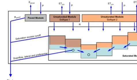
The model consists of three separate, linked modules (Fig. 2):
1. The paved area module is a lumped and conceptual model that calculates runoff and evaporation from paved areas.
2. The unsaturated zone module calculates recharge from the unsaturated zone to the saturated zone, preferential flow that bypasses the unsaturated zone and directly en-ters the saturated zone, and evapotranspiration from the unsaturated zone. It is possible to have several unsatu-rated zone modules (e.g., one for each soil type), each of which recharges into different sections of the saturated zone module.
3. The saturated zone module is spatially distributed (grid cells) and more process-based. It simulates lateral groundwater flow, drain flow, evapotranspiration from the saturated zone, and saturation-excess overland flow. The concept of the saturated zone module was inspired by HillVi (Weiler and McDonnell, 2004).
The modeled stream discharge consists of the following components:
Q=Qpaved+Qsurf+Dlat+Dpref, (3) whereQpaved [L T−1] is runoff from the paved area,Qsurf [L T−1] is saturation excess surface runoff (this term also comprises lateral groundwater flow to the stream, see below), Dlat [L T−1] is lateral drain flow, andDpref[L T−1] is pref-erential drain flow.
The modeled evapotranspiration is calculated as follows:
ET=Epaved+ETuns+ETsat, (4)
whereEpaved [L T−1] is the evaporation from paved areas, ETuns[L T−1] is the evapotranspiration from the unsaturated zone, and ETsat [L T−1] is the evapotranspiration from the saturated layer. In the following the three modules are de-scribed in detail.
Paved Module Unsaturated Module
Soiltype 1
Unsaturated Module
Soiltype 2 P
Discharge
Epaved ET
uns
Rpaved
Saturation excess runoff
Drainflow, lateral and prefer ential
R
Saturated Module
ETuns
P P
[image:6.612.307.545.67.206.2]ETsat
Figure 2. Schematic picture of the model concept.
Paved area module
The change in the paved storage is modeled as follows: dSpaved
dt =P−Epaved−Qpaved, (5)
withSpaved[L] being the paved storage.
Runoff from paved areas linearly depends on the paved storage.
Qpaved= (6)
(
0 if Spaved≤Spaved_min
(Spaved−Spaved_min)kpaved if Spaved> Spaved_min Spaved_min[L] is the minimum storage that has to be filled to produce runoff andkpaved[T−1] is the outflow rate.
If there is water in the paved storage, it can evaporate with the following rate
Epaved=ETref·mpaved, (7)
where ETref[L T−1] is the reference evapotranspiration cal-culated from meteorological data (see Sect. 2.2), andmpaved [–] is a multiplier.
Unsaturated zone module
The water balance of the unsaturated zone is represented as follows:
dSuns
dt =P−ETuns−R, (8)
whereSuns[L] is the unsaturated storage, andR [L T−1] is recharge to the saturated zone.Rconsists of a slow recharge component (Rslow) and preferential flow (Rpref).
R=Rslow+Rpref (9)
Rslowis assumed to be zero.
Rslow=
(
0 if Suns< Sfc
(Suns−Sfc)kuns if Suns≥Sfc (10) Sfc[L] is the unsaturated store at field capacity andkuns[T−1] is the outflow rate.
A part of the precipitation bypasses the unsaturated zone as preferential flow and directly enters the saturated zone. This only occurs if the unsaturated zone is above field capac-ity, and it exponentially depends on the water content in the unsaturated zone.
Rpref=
(
0 if Suns< Sfc
kpref
Suns−Sfc
Suns_max−Sfc
epref
·P if Suns≥Sfc
(11)
kpref[–] andepref[–] are empirical parameters.
Above field capacity the evapotranspiration from the un-saturated module is at maximum, below field capacity it is reduced. The reference evapotranspiration calculated from meteorological data (ETref) refers to a reference grass sur-face. A time dependent multiplier (muns) was introduced to account for crops with different water requirements and the time dependence of the leaf area index (LAI) due to crop de-velopment.
ETuns= (12)
ETref·muns if Suns≥Sfc
ETref·muns
Suns
Sfc Suns
Sfc+ket
(1+ket) if Suns< Sfc
withket [–] andmuns [–] being parameters. The change of the LAI is coupled to air temperature and incorporated in the time dependent parametermuns.
dmuns
dt = (13)
muns·µ0(Tair−T0)1− muns
muns, max
if Tair≥T0 muns·kdecay(Tair−T0) if Tair< T0
0 if muns≤muns, min
,
whereµ0[T−1Te−1] andkdecay [T−1Te−1] are parameters, Tair[Te] is air temperature,T0[Te] is the minimum temper-ature above which LAI starts increasing, muns, min [–] and muns, max[–] are the minimum and maximum values formuns. Saturated zone module
The saturated module is spatially distributed. The water bal-ance within a grid-cell is calculated as follows:
dSsat
dt =R−ETsat+SFlat−i·Dlat−i·Dpref−j·Qsurf, (14)
whereSsat[L] is the storage in the cell and SFlat [L T−1] is the lateral groundwater flow between cells.
i=
(
1 for drained cells
0 for undrained cells (15)
j=
1 for cells with surface connectivity to the stream, see Sect. 2.3
0 for cells without surface connectivity to the stream
(16)
The change of the groundwater level in the cell is therefore calculated as follows
dh dt =
dSsat dt
peff, (17)
whereh[L] is the groundwater level andpeff[–] is the effec-tive porosity.
If the unsaturated zone is below field capacity and evap-otranspiration from the unsaturated zone is therefore re-duced, evapotranspiration can occur directly from the satu-rated zone.
ETsat=
(
0 if Suns≥Sfc
msat(ETref·muns−ETuns) if Suns< Sfc
(18) At maximum, ETsat accounts for the evapotranspiration deficit in the unsaturated zone, the multipliermsat[–] is be-tween 0 and 1.
The lateral groundwater flow between cells is calculated based on the Dupuit–Forchheimer assumption. We further-more assume isotropy inKsat:
qlat=Ksat· ∇h, (19)
whereqlat[L T−1] is the flux density,Ksat[L T−1] is the sat-urated hydraulic conductivity, andh[L] is the groundwater head. The water flow between two neighboring cells can then be calculated as follows:
Qlat=Ksat·Msat·Lcell 1h
Lcell, (20)
whereQlat[L3T−1] is the water flow between two cells,Msat [L] is the thickness of the saturated layer, andLcell[L] is the cell length. If we sum up the water flows to and from all neighboring cells and divide the sum by the cell area, we receive SFlat.
In drained cells, the lateral groundwater flow into the drain is calculated based on the Hooghoudt equation as de-scribed by Beers (1976). We used an equation modified from Wittmer (2010) because the distance to single tiles is not con-sidered explicitly. The flow depends on the water level above the drains.
Dlat=4rdr·Ksat
mdr·Hdr Spdr
2
Dlat [L T−1] is the drain flow,rdr[–] is a parameter that de-termines the entrance resistance to the tile drains,mdr[–] is a multiplier to obtain the water level in the middle between two drains from the modeled water level in the cell,Hdr [L] is the water table height above the drain, and Spdr[L] is the drain spacing.
If the groundwater level reaches the surface in a cell, three cases are distinguished:
1. The cell is directly connected to the stream on the face (see Sect. 2.3). In this case all water above the sur-face is directly added to discharge (Qsurf).
2. The cell is not connected but it is drained. In this case, all water above the surface is added to drain flow as pref-erential flow (Dpref).
3. The cell is neither connected to the stream nor drained. The water remains in the cell.
The coupling between the saturated zone module and the un-saturated zone module is unidirectional from the unun-saturated zone to the saturated zone. The fact that a cell is saturated to the surface does not influence the unsaturated zone module above it. It is possible that the unsaturated zone above a satu-rated cell is not completely full. This concept was chosen to achieve a high computational efficiency.
The stream channel cells are incised to a mean water level in the stream. The surface topography in the stream cells is therefore represented by the mean water level and all the wa-ter above this level in the cell is directly converted to dis-charge. Lateral groundwater flow to stream cells is therefore also converted toQsurf.
2.5.2 Model setup
We ran the model with homogeneous hydraulic properties in the saturated zone; only topography and the presence of tile drains were spatially distributed. The unsaturated zone was divided into several classes according to land use (for-est, settlement, agriculture) and, within agricultural land use, according to the seven soil categories (see Sect. 2.4). We therefore ended up with nine unsaturated zone classes (for-est, settlement and the seven soil categories). The reason for this setup was the assumption that the groundwater level in the catchment is mainly influenced by topography and artifi-cial drainage and not by hydraulic soil properties (soil texture is rather homogeneous within the catchment, FAL, 1997). However, to account for the spatial distribution of the unsatu-rated zone thickness (which also influences the other param-eters of the unsaturated zone module), we divided the unsat-urated zone into classes according to their soil water regime. The classification of soil water regimes was only used for the spatial division of the unsaturated zone (but not its parame-terization).
The saturated zone was represented by a 16 m×16 m grid; the cells were 10 m thick. We assume that the soil and the
moraine are the conducting layers while the Fresh water mo-lasse is assumed to be impermeable (see Sect. 2.1). The cal-culations were run with hourly input time series; the model output was also in hourly steps.
2.5.3 Implementation
The model equations were implemented in a C++ program to achieve fast model simulations. The ordinary differential equations of the conceptual unsaturated zone modules and the paved area module were numerically integrated with the LSODA solver package (Livermore Solver for Ordinary Dif-ferential Equations, Hindmarsh, 1983; Petzold, 1983). The partial differential equations of the saturated zone module were integrated with an explicit Euler solution scheme with a computational time step (20 min) that guaranteed numer-ical stability during the simulation period. The integration of the saturated zone module was sped up by paralleliz-ing the explicit solution scheme with OpenMP threads (for the specification see http://openmp.org). Despite all these ef-forts the simulation of the 2-D groundwater surface remained rather time consuming requiring 28 s of computation time for 1 yr of forward simulation on an Intel Core i7–3960X CPU (3.3 GHz).
Model implementation and model setup (e.g., spatial and temporal resolution) were chosen in a way that guaranteed simulations fast enough to allow a possible use for practical applications.
2.5.4 Calibration
The model was simultaneously calibrated to the discharge time series and the groundwater level time series in the eleven piezometers. A maximum likelihood approach was used. Discharge was Box–Cox transformed before calibra-tion withλ=1/3 (Box and Cox, 1964, 1982). The transfor-mation equation was as follows:
g(x)=x
λ−1
λ (22)
This was done to reduce heteroscedasticity of discharge rors. We assumed independent and normally distributed er-rors for the transformed discharge and the (untransformed) groundwater levels; the individual standard deviations for these were also calibrated. The likelihood function therefore looked as follows:
L(θ,σ)∝
11
Y
i=1
m Y
j=1 1 σi
√
2πexp
−
1 2
Oij−Mij(θ) σi
!2
(23)
×
m Y
j=1 1 σd
√
2πexp
−
1 2
g(Odj)−g(Mdj(θ)) σd
!2
,
11 piezometer locations,jare the time points,σiis the
stan-dard deviation at piezometeri,Oij is the observed ground-water level at piezometer iand time j,Mij(θ)is the mod-eled groundwater level at piezometeriand timej,σdis the standard deviation of the transformed discharge,g(x)is the Box–Cox transformation (Eq. 22), and Odj is the observed discharge at time j andMdj(θ)is the modeled discharge at timej.
When calibrating a grid cell model to piezometer mea-surements, one has to be aware of the difference in spatial support. The model cell represents an area of 16 m×16 m while the piezometers are point measurements. The spatial variability of groundwater levels within each model cell can therefore be considerable (see e.g., Freer et al., 2004) and this variability cannot be resolved by the model. This is es-pecially true for drained areas, where the tile drains increase the spatial variability of groundwater levels.
In the context of multi-objective calibration our approach corresponds to a simple aggregation function (Efstratiadis and Koutsoyiannis, 2010) for combining the different state variables into a single objective function where the trade-offs between the different objectives are not made explicit. The weighting of the different state variables in the objec-tive function was done by using individual error variances for each state variable (Reichert and Schuwirth, 2012). These error variances were also calibrated as parameters within the optimization. Hence, the optimization algorithm was allowed to choose the weighting that has the maximum likelihood. Implications of this approach will be discussed in the discus-sion section.
During calibration the likelihood function was opti-mized with a coupled global–local algorithm. Optimization started with the Particle Swarm algorithm (Kennedy and Eberhart, 1995) and after reaching the stop criterion Nelder– Mead Simplex optimization (Nelder and Mead, 1965) was launched from the best parameter combination.
We chose a period in spring and summer 2009 as cali-bration period. It starts very wet in the beginning of spring, includes a long dry period, several rain events with varying magnitudes and intensities and it also contains the largest dis-charge event in the measurement period. We do not have con-tinuous measurement time series from all the piezometers. For each piezometer we chose the calibration period so, that all the calibration time series (discharge and the 11 piezome-ters) contained the same number of observations. With this, the weighting of the different state variables within the ob-jective function only depends on their error variance and not implicitly on the number of observations used for calibration. For piezometers 10 and 11 no data were available in the later period, so their calibration period is partially within the warm up phase of the model. Even though this might be problem-atic because we calibrate the model in a state where it is not yet completely adapted to the parameter set, we kept these two piezometers in the calibration. The main reason for this
was that they are the two piezometers with the lowest ground-water levels and are therefore important for a complete spa-tial picture of the groundwater surface in the catchment. This more complete spatial picture was of greater importance to us than the potentially problematic calibration in the model warm up period.
Most of the model parameters were calibrated to achieve the best possible model output with the given model struc-ture. (The Tables S1 to S4 in the Supplement indicate which of the parameters were calibrated and which were kept fixed during calibration. The tables also indicate the minimum and maximum values that were allowed in the calibration.) The initial state of the unsaturated zone was calibrated as well. The initial condition for the groundwater level is difficult to calibrate because the shape of the surface depends on the model parameters. The model run was started 5 months be-fore the calibration period to adapt the groundwater surface to the model parameters. Additionally, we added a param-eter that allows a homogeneous shifting up or down of the groundwater initial state and chose an adaptive procedure. After a first calibration, we used a groundwater level map from the optimum parameter set as initial condition for a sec-ond calibration. In a first step we calibrated a model version with a homogeneous unsaturated zone. From the resulting optimum parameter set, we launched the calibration of the model version with the spatially distributed unsaturated zone. With this setup, one full optimization (global and local) took about 1 week, depending on the speed of convergence.
3 Results
3.1 Saturation estimates
( 1
m
0HWHUV 6RLOJURXS 0DLQ URDG6WUHDP LQ FXOYHUW
2SHQ 6WUHDP &DWFKPHQW ( 1
m
0HWHUV 7RSRLQGH[ +LJK /RZ 0DLQ URDG 2SHQ 6WUHDP6WUHDP LQ FXOYHUW
&DWFKPHQW ( 1
m
0HWHUV 0DLQ URDG 2SHQ 6WUHDP6WUHDP LQ FXOYHUW &DWFKPHQW
'UDLQHG DUHD
B
A
C
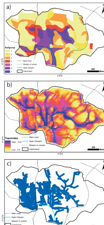
Figure 3. (a) The reclassified soil map with the seven soil water
regime classes (class 1 is the driest, class 7 the wettest), (b) map of the topographic wetness index, (c) map of the drained areas in the catchment. Sources: Gemeinde Ossingen (1995); swisstopo (2008).
classified the wettest 20 % as CSA. The areal overlap of the CSAs from the two methods is 52 %. Despite this reasonable agreement between the two maps there are some areas with rather high topoindices where the soils are classified in dry soil classes (e.g., in the west of the catchment).
The location of tile drains also contains information on the soil water regime. The tile drain map can therefore be used as additional comparison to verify the soil map esti-mates. Tile drains are only present at locations with excess groundwater that has to be diverted. Drained areas are there-fore good indicators of originally higher groundwater levels. Because the drains are installed between 1 and 1.5 m below
● ● ● ● ● ● ● ● ● ● ● ● ● ● ● ● ● ●
Water regime class 1
−2 −1 0 ● ● ● ● ● ● ● ● ● ● ● ● ● ● ● ● ● ●
Water regime class 2
−2 −1 0 ● ● Best guess
±Std. dev. Piezometer ● ● ● ● ● ● ● ● ● ● ● ● ● ● ● ● ● ●
Water regime class 3
−2 −1 0 ● ● ● ● ● ● ● ● ● ● ● ● ● ● ● ● ● ●
Water regime class 4
Depth belo w surf ace [m] −2 −1 0 ● ● ● ● ● ● ● ● ● ● ● ● ● ● ● ● ● ●
Water regime class 5
−2 −1 0 ● ● ● ● ● ● ● ● ● ● ● ● ● ● ● ● ● ● Water regime class 6
−2 −1 0 ● ● ● ● ● ●
0 20 40 60 80 100
● ● ● ● ● ● ● ● ● ● ● ● Water regime class 7
Fraction of time [%]
−2
−1
[image:10.612.68.266.64.491.2]0
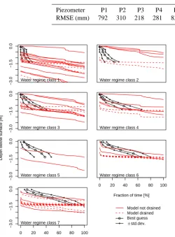
Figure 4. The estimated depth dependent saturation durations in the
seven water regime classes with the expected variation within each class (blue) together with the measured saturation duration in the piezometers (black).
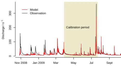
[image:10.612.338.519.67.433.2]Time
Discharge l s
−
1
Nov 2008 Jan 2009 Mar May Jul Sept
0
100
200
300
Model Observation
[image:11.612.310.545.64.248.2]Calibration period
Figure 5. The modeled and measured discharge time series.
other three soil pits (Fig. 1) the piezometric measurement, the local morphological interpretation in the soil pit and the map-based estimate corresponded well.
3.2 Calibration results and model validation
After calibration (the optimum parameter set can be found in Tables S1 to S4 in the Supplement), the model performed satisfactory with respect to discharge and absolute ground-water levels. Figure 5 shows the predicted and measured dis-charge time series. The bad fit in the beginning stems from the difficulty to calibrate the initial groundwater level (see Sect. 2.5.4). After this initial phase, the discharge prediction is good with a Nash–Sutcliffe coefficient (Nash and Sutcliffe, 1970) of 0.91 for the calibration period. Also the predicted average groundwater levels at the piezometer locations are in good agreement with the measurements (Table 1). After the initial phase, the root mean square error (RMSE) of the groundwater level prediction ranged between 22 cm and 1 m with a median of 41 cm (Table 1). The model was there-fore able to reproduce the general hydrological behavior of the catchment. The modeled composition of the discharge, with most of the discharge originating from the drainage sys-tem, was also in satisfactory agreement with the measure-ments: the model attributed 82 % of total discharge to dis-charge from tile drains, while we estimate 62 % based on the measurements.
However, if the time series of the groundwater levels are plotted as depth below the soil surface (Fig. 6) it becomes ob-vious that there is a lack of groundwater level dynamics in the model. The observed groundwater levels are much more dy-namic than the modeled ones. Additionally, Fig. 6 shows that the depth to groundwater in the model prediction is rather ho-mogeneous throughout the area. The modeled average depth to groundwater does not vary much between the piezometer locations. In contrast, the measured depth to groundwater is more variable.
To further investigate the model performance with respect to the spatial distribution of groundwater levels we used the estimated saturation durations from the soil map (Fig. 7).
out$jul
−3.0
−1.5
0.0
out$jul
out$gw13
1 1
out$jul
out$gw2
2 1 D
out$jul
out$gw60
3 7
out$jul
−3.0
−1.5
0.0
out$jul
out$gw56
4 7 D
out$jul
out$gw52
5 7
out$jul out$gw43_1 7 D 6
out$jul
−3.0
−1.5
0.0
out$jul out$gw43_2 7 D 7
Depth belo
w surf
ace [m]
out$jul out$gw43_3 4 D 8
out$jul
out$gw49
9 3 D
Jan 2009 July
out$jul
−3.0
−1.5
0.0
out$jul
out$gw62
10 1
Jan 2009 July
out$jul
out$gw33
11 2
Jan 2009 July
out$jul
out$gw2
Calibration period
Model Observation
Figure 6. The modeled and measured groundwater levels at the
piezometer locations as depth from the surface. The individual cal-ibration periods are indicated (see Sect. 2.5.4). The circled number is the piezometer location (Fig. 1), the number in the colored box shows the water regime class, D indicates a drained model cell.
This allowed a model evaluation at locations without mea-surements and at locations where the model was not cali-brated to. The number of evaluation cells in each soil type was chosen according to the area covered by the correspond-ing soil type. The evaluation cells were selected in the center of the soil types to avoid influence from the boundaries. Fig-ure 7 shows that the model does not differentiate between the water regime classes. In all the classes, there are dry and wet model cells. The underestimation of variability is a general behavior, dry locations (water regime class 1) are too wet, and wet locations (water regime classes 6 and 7) are too dry in the model. However, the model was able to predict the ar-eas with the lowest groundwater levels. Model cells where the modeled groundwater level is deeper than 3 meters be-low the surface are only located in water regime class one (Fig. 7). Hence, the model was not able to reproduce the spa-tial variability in saturation durations, except for the locations with the lowest groundwater levels, even though it was cali-brated on measured groundwater levels distributed through-out the catchment.
[image:11.612.49.283.65.197.2]Table 1. Deviations between observed and simulated water table levels in the 11 piezometers.
Piezometer P1 P2 P3 P4 P5 P6 P7 P8 P9 P10 P11 RMSE (mm) 792 310 218 281 832 857 1001 328 441 411 1003
● ● ● ● ● ● −3.0 −1.5 0.0 ● ● ● ● ● ● ● ● ● ● ● ●
Water regime class 1
● ● ● ● ● ● ● ● ● ● ● ● ● ● ● ● ● ●
Water regime class 2
● ● ● ● ● ● −3.0 −1.5 0.0 ● ● ● ● ● ● ● ● ● ● ● ●
Water regime class 3
● ● ● ● ● ● ● ● ● ● ● ● ● ● ● ● ● ●
Water regime class 4
● ● ● ● ● ● −3.0 −1.5 0.0 ● ● ● ● ● ● ● ● ● ● ● ●
Water regime class 5
Depth belo w surf ace [m] ● ● ● ● ● ● ● ● ● ● ● ● ● ● ● ● ● ●
Water regime class 6
0 20 40 60 80 100
Fraction of time [%]
● ● ● ● ● ● −3.0 −1.5 0.0 ● ● ● ● ● ● ● ● ● ● ● ●
Water regime class 7
0 20 40 60 80 100
Fraction of time [%]
Model not drained Model drained
●
●
Best guess
±std.dev.
Figure 7. Comparison of the depth distribution of the saturation
du-ration in selected model cells with the estimate from soil morphol-ogy. The model results are grouped into the respective water regime class and into drained and not drained cells.
the pattern observed in soil morphology. The spatial over-lap between wet areas as estimated from the soil map (water regime classes 6 and 7) and the wettest 20 % of the cells in the modeled output is only 12 %. Model and soil map would therefore predict completely different locations as CSAs. The model predicts high water tables in areas where it should be dry. In the center of the catchment, where the area is drained but still wet in reality, the model predicts too low water levels (compare Fig. 8 with Fig. 3c). It seems that the drainage sys-tem in the model is too efficient in lowering the groundwater table.
4 Discussion
4.1 Soil map translation
A meaningful validation of the saturation duration estimates from the soil map is not straightforward due to several
8°44'E 4 7 °3 7 'N
±
200 MetersDepth to GW
[m]
0 - 0.2 0.2 - 0.4 0.4 - 0.6 0.6 - 1 1 - 1.4 1.4 - 2 > 2
Main road
Stream in culvert
Open Stream
[image:12.612.53.304.82.422.2]Catchment
Figure 8. Map of the modeled depth to groundwater on
27 July 2009.
difficulties. First, the spatial coverage of the estimates corre-sponds to the soil map unit while piezometers are point mea-surements. Hence, deviations between soil map estimates and piezometer data may simply reflect local heterogeneities. Furthermore, the soil map divides the area into units with sharp boundaries. Some of these boundaries are in reality gradual changes. The vicinity of a piezometer to a soil unit boundary (especially boundaries between very wet and very dry soils) can therefore complicate a meaningful evaluation. A second difficulty is that the estimates do not differ heav-ily; the saturation estimates change gradually from one class to the next. The piezometer measurements could therefore fit well in more than one class. Third, there are temporal as-pects of the validation. Soil morphology does not necessarily reflect the current water regime, especially when the water regime has recently changed because of artificial drainage. According to Hayes and Vepraskas (2000), soil drainage can alter morphology within decades. Finally, it is possible that the morphological signs of wetness do not evolve in a cer-tain soil, even though the same water regime has persisted a longer time. A possibility for this is soil saturation without oxygen depletion (e.g., frequent but short periods of satura-tion), which does not lead to morphological changes (Evans and Franzmeier, 1986; Pickering and Veneman, 1984).
[image:12.612.301.548.87.303.2]The mismatch between the measured groundwater level and soil morphology at piezometer 1 shows the limitations of the approach. Soil morphology does not reflect the cur-rent water regime everywhere. As stated above, it is possi-ble that the morphological signs of wetness did not evolve in this soil, even though the same water regime has persisted a longer time. On the other hand, the current water regime as measured in the piezometer could have developed only few years ago for several reasons, possibly because of a poorly maintained and clogged part of the drainage system, for ex-ample.
Despite these difficulties and limitations, the comparison of the estimates with the piezometric measurements shows a generally good agreement (Fig. 4). We are therefore con-fident that soil morphology in this region reflects the cur-rent water regime in most soils. The good agreement between the topographic wetness index and the map of the soil water regime classes indicates that the soil distribution with respect to soil saturation and soil water regime is strongly driven by topography in this catchment. In addition, this correspon-dence shows that the estimation of soil saturation from soil map information resulted in a reasonable spatial pattern of soil saturation in this catchment.
The quantitative interpretation of soil morphology will al-ways remain uncertain to some degree. However, if the un-certainties can be quantified, such information can still be very valuable for model calibration and evaluation (Franks et al., 1998).
4.2 Model predictions 4.2.1 Calibration
We chose a model setup with a homogeneous saturated zone because the geological map does not indicate any spatial dif-ferentiation (swisstopo, 2007). Also soil texture in the study catchment is rather homogeneous. In addition, the soil tex-ture classes in the Swiss classification system (FAL, 1997) are rather wide. Therefore, a spatial distribution based on geological information or texture information obtained from the soil map would not have resulted in much variability. The only spatially variable attributes in the saturated zone mod-ule were surface topography, surface connectivity and the ex-istence of tile drainage. However, the unsaturated zone was spatially differentiated based on the water regime classes be-cause we expect different thicknesses of the unsaturated zone in the water regime classes. This setup resulted in 83 pa-rameters to be calibrated. Parameter optimization was there-fore a rather complex problem with the simultaneous cali-bration to discharge and groundwater levels at 11 locations. We started the calibration at the optimum parameter set of a model setup with a homogeneous unsaturated zone. Some of the parameters did not differentiate into the nine unsatu-rated zones but remained at the starting parameter value for all or some of the soil types. The likelihood function was
therefore insensitive to a spatial distribution of these param-eters (these paramparam-eters are indicated in Tables S1 to S4 in the Supplement).
It could be argued that the poor model performance re-garding water table levels is caused by a wrong subjective at-tribution of weights to the water table data in the aggregating likelihood function (Efstratiadis and Koutsoyiannis, 2010) (Sect. 2.5.4). Because we used such a single function we did not explicitly quantify the trade-offs between discharge and water table simulations. An imbalance in the weighting could be caused (i) by an unbalanced number of data points for the different variables or (ii) a disparity between the stan-dard deviations attributed to the variables in the likelihood function (Eq. 23). The first possibility is excluded because the actual number of piezometric data exceed the discharge data by a factor of 11 (Sect. 2.5.4). The second possibility was avoided by the joint calibration of the standard devia-tions. We chose wide priors for all the error variances, so we did not force the model into a solution where only discharge was reproduced well. Hence, if there was a parameter set that performed well on some of the water table levels – causing the standard deviation to be small – it had outperformed data sets that performed only well on discharge.
Based on the arguments above we do not believe that the rather poor model performance with respect to groundwater level dynamics can be attributed to problems related to the chosen calibration procedure. We rather think that the prob-lems arise from the model structure.
better choices than the independence assumption. However, in contrast to the width of predictive uncertainty interval and parameter values, the maximum likelihood fit for discharge series was often proven to be robust against neglecting the autocorrelation in residuals (Honti et al., 2013; Del Giudice et al., 2013). The large variability in the shape of the resid-ual distributions and in the extent of autocorrelation suggests that – in a next calibration exercise – individual distributions and individual autoregressive errors should be assumed for the piezometers.
4.2.2 Model performance
The model is able to reproduce the general hydrological be-havior of the catchment (Fig. 5 and Table 1). The satisfactory match between observed and modeled groundwater levels with a model that assumes homogeneous soil properties in-dicates that groundwater levels in this catchment are mainly driven by topography and are not strongly influenced by the variability of hydraulic soil properties. However, if we focus on the top two meters below soil surface there are deficien-cies in the groundwater level predictions.
The comparison with the estimates of soil saturation re-veals a lack of differentiation between wet and dry areas (Fig. 6) and wrong spatial patterns of soil saturation (Fig. 8). The main problems are (i) the missing dynamics in the groundwater levels, (ii) the dominance of the drainage sys-tem with respect to groundwater levels which leads to wrong spatial patterns of soil saturation and (iii) the homogeneity within the drained part of the catchment. These deficiencies are problematic if one wants to use such a model to predict critical source areas. Saturation-excess overland flow only occurs in situations with high groundwater levels. A pdiction model therefore needs to be able to adequately re-produce groundwater dynamics especially in situations with high groundwater levels. Furthermore, large parts of the in-tensively cultivated cropping areas in Switzerland are artifi-cially drained; the model should therefore be able to predict groundwater levels and their dynamics in drained areas. The prediction of saturation excess areas requires a very high ac-curacy in groundwater level prediction. A difference of 50 cm or less in the depth to groundwater is already crucial, because it decides whether an area often produces saturation-excess overland flow. Even though the model captured the general hydrological behavior of the catchment with respect to dis-charge and absolute groundwater levels, it was far from be-ing useful as a prediction tool for saturated areas. It did not achieve the accuracy that is needed for practical applications. Some of the deficiencies in water level dynamics were possibly caused by the chosen model structure. The current model only considers the effects of different antecedent soil moisture contents within the unsaturated zone. This influ-ences the recharge to the saturated zone. However, within the saturated zone, antecedent soil moisture is neglected (con-stant effective porosity) and therefore has no influence on the
increase of the water table during different events. Further-more, effective porosity is the same during rising and falling water tables in the model. In reality however, the amount of water needed to increase the water level by a given level de-pends on the degree of saturation before the event. Addition-ally, the degree of saturation above a rising water table does not need to be the same than the degree of saturation above a falling water table. This can only be achieved by coupling the soil moisture dynamics in the unsaturated zone and the groundwater level dynamics in the saturated zone.
Because crops may differ strongly in their water require-ments at any given moment, accounting for antecedent soil moisture may require the inclusion of crop specific water ab-straction from the unsaturated zone. This may be actually a reason why the relative responses of the water table in differ-ent piezometers differed between evdiffer-ents.
A further problem is the representation of the drainage sys-tem, which is a dominant feature in the hydrology of the catchment. Because most of the area has no direct connec-tion to stream, i.e., surface runoff cannot directly reach the stream (Doppler et al., 2012), we know that most of the dis-charge reaches the water course through tile drains. At the same time, we know that the water table is often quite close to the soil surface despite the efficient drainage of the water through the soil. The current model version drains the soils too efficiently. In order to get as much water as possible dur-ing rain events through the soil while keepdur-ing the water table at a higher water level it is obvious that the water flux has to increase more strongly (in nonlinear fashion) with the wa-ter table than described by Eq. (21). Conceptually, this could be achieved by adding an additional preferential flow com-ponent that depends (in a nonlinear manner) on the current water level (see Frey et al., 2011, for a similar solution).
Especially in drained areas it is important to be aware of the difference in spatial support between piezometer readings and model predictions. Piezometers are point measurements while the model predictions are made on a 16 m×16 m grid. The tile drain spacing is around 15 m. So the model does not resolve the difference between locations directly above tile drains and locations in the middle between tile drains. In reality however, this difference is important with regard to groundwater levels. If a piezometer is directly above a tile drain, the model would overestimate its groundwater level. But it would underestimate groundwater levels in between tile drains.
reproduction of very steep gradients on short distances which also influences the groundwater level dynamics.
Based on the available information on geology (swisstopo, 2007) and soil texture (FAL, 1997) there was no indication to spatially distribute the parameters of the saturated zone (see Sect. 4.2.1). If there was a parameter set within our model structure that would perform well on some of the piezome-ters (because the saturated zone paramepiezome-ters fit well for this soil type), this parameter set would have outperformed other solutions. But the maximum likelihood parameter set does not well reproduce groundwater level dynamics (especially in the peaks) of any piezometer. We do therefore believe that this rather poor model performance has to be attributed to the model structure and not to the calibration procedure or lack of spatial heterogeneity in the model.
A closer look at the piezometer data in Fig. 6 reveals that the level fluctuations of the shallow groundwater are rather complex even in the rather simple and homogeneous study catchment. Every piezometer reacts individually to the dif-ferent rain events. Moreover, the dynamics of piezometers within the same water regime class differ substantially. Even if we consider whether a piezometer location is drained or not, it is impossible to explain the differences and similarities of the groundwater dynamics. It would have been possible that the model can explain the spatial variability of ground-water level dynamics if these dynamics are determined by a combination of topographic position, the soil water regime class and the drained areas. However, the discrepancy be-tween modeled and measured groundwater levels indicates that other processes influence the groundwater levels to a de-gree that cannot be neglected. From a scientific point of view it would be interesting to dig deeper into these processes, try-ing to understand the influenctry-ing factors of the groundwater level dynamics. To do so, we suggest using a model with a more detailed representation of the processes at the bound-ary between the saturated and the unsaturated zone and a more realistic description of the drainage system. The for-mer could possibly be achieved within a conceptual model as it was done by Seibert et al. (2003). The latter however, would require a spatially explicit drainage system represen-tation with high spatial resolution. Such a model would need detailed information on the drainage system and its mainte-nance status, which is often not available.
In the light of the above discussion about a model that in-cludes additional processes, it seems surprising that the spa-tial pattern of wet areas as predicted by the topographic wet-ness index is in better agreement with the soil map than the predictions of the more complex model (Figs. 3 and 8). A comparison to TOPMODEL predictions could therefore be interesting. According to TOPMODEL, the spatial ground-water level distribution is simply dependent on the distribu-tion of the wetness index and the average moisture level in the catchment. At each location there is a constant offset to the mean depth of the water table in the catchment that de-pends on the deviation between the local wetness index and
● ●
●
●
●
●
●
●
● ●
●
7 8 9 10 11 12 13
−2.5
−2.0
−1.5
−1.0
−0.5
Topographic wetness index
Groundw
ater le
v
el [m belo
w surf
ace]
2 1
11
6
7
8 9
5
4 3
[image:15.612.334.522.62.234.2]10
Figure 9. Average groundwater depth in the piezometers as a
func-tion of the local wetness index. Numbers refer to the piezometer number, colors to the corresponding soil water regime class.
its average value (Blazkova et al., 2002). Accordingly, one would expect the depth of the water table to be correlated with the local wetness index. Figure 9 depicts the average water level as a function of the wetness index. It is obvi-ous that for low index values there is a large scatter of the data and for high index values the water table hardly depends on the index. We used a topographic wetness index that ne-glects local transmissivity. However, using a wetness index including transmissivity estimated from soil map informa-tion (as introduced by Beven, 1986) would not significantly change the spatial pattern because of the homogeneous soil texture and geology in the catchment (see above). Hence, a simple wetness index based approach does not outperform our model approach.
This conclusion is supported by the comparison of the dy-namics of the different piezometers. According to the TOP-MODEL approach, the water table dynamics at different to-pographical positions should simply be shifted in height of the water table (if one assumes a constant drainable poros-ity with depth). Figure 6 however, reveals that the dynamic varies substantially between the piezometers. Our approach mostly failed to reproduce these differences; conceptually TOPMODEL will do so as well.
models based on generally available information and – from a practical perspective – once they are identified in the field there is no need to implement them into a prediction model.
The focus of this study was to use a model that would be applicable for practical purposes. Besides model-based pre-dictions, critical source areas can also be directly identified in the field by experts. This requires interviews with the local farmers and detailed site inspections. If a prediction model for CSAs should serve as basis for pollution mitigation mea-sures, it must have advantages as compared to field visits by experts. An advantage of model predictions would be that predictions can be based on existing knowledge, so that field visits would not be necessary. However, the need for very de-tailed knowledge (e.g., on the drainage system and on the ac-tual land management) cancels this advantage. Additionally, the demanding setup of a very detailed model, its calibration, and tests in every small catchment (not to mention uncer-tainty analysis), would not lead to a time gain compared to field visits by experts to directly identify CSAs in the field.
5 Conclusions and outlook
Our case study has shown that the estimation of saturation durations from morphological soil map information is possi-ble and these estimates have proven to be useful for model validation even though the resulting map of duration of soil saturation remains uncertain to some degree because the esti-mates do not always represent the current water regime. The additional data source provides quantitative spatial informa-tion on the soil water regime that can be used as validainforma-tion data for the predicted spatial patterns. In a further step such estimates could also be used to calibrate spatially distributed hydrological models, so that no groundwater level measure-ments are needed for model calibration.
The model was able to reproduce the general hydrological behavior of the catchment. However, the desired accuracy of the groundwater level predictions – which is needed for the identification of CSAs – could not be achieved. The pro-cesses that determine the groundwater level dynamics in this catchment seem to be more complex than the used model. It seems that a high spatial resolution and detailed process representations are needed for a groundwater level predic-tion that is accurate enough for the identificapredic-tion of CSAs in practical situations. Drained areas are especially challeng-ing for the followchalleng-ing reasons: limited data availability on tile drain locations and maintenance status, difficult integration in catchment models (concept and spatial resolution), and fi-nally the estimation of soil saturation duration is much more difficult in drained areas.
Our results indicate that dynamic, spatially distributed hy-drological models to predict CSAs are still far from being useful for management decisions. If a model should be accu-rate enough and should also include infiltration excess areas, it would require information that is not generally available.
Furthermore, the setup and test of such a complex model would need more resources than direct observations of CSAs in the field by experts and the local farmers. If site specific management of CSAs should be achieved, we recommend identifying these areas in the field and not solely by model predictions. However, predictions by simple models like the topographic wetness index can be helpful for the identifica-tion of CSAs in the field. It would also be interesting to test the predictive capabilities of different modeling concepts un-der real world conditions.
The Supplement related to this article is available online at doi:10.5194/hess-18-3481-2014-supplement.
Acknowledgements. The field work would not have been possible
without Ivo Strahm, Luca Winiger, Marcel Gay and Hans Wunderli. We also would like to acknowledge the local farmers for their cooperation. Comments by the referees significantly improved the quality of the manuscript. We gratefully acknowledge the funding by the Swiss Federal Office for the Environment (FOEN). Edited by: J. Freer
References
Abbott, M. B., Bathurst, J. C., Cunge, J. A., O’Connell, P. E., and Rasmussen, J.: An introduction to the European Hydrological System – Systeme Hydrologique Européen, “SHE”, 1: history and philosophy of a physically-based, distributed modelling sys-tem, J. Hydrol., 87, 45–59, 1986.
Agnew, L. J., Lyon, S., Gérard-Marchant, P., Collins, V. B., Lembo, A. J., Steenhuis, T. S., and Walter, M. T.: Identifying hydrologically sensitive areas: bridging the gap between science and application, J. Environ. Manage., 78, 63–76, 2006.
Allen, R. G., Pereira, L. S., Raes, D., and Smith, M.: Crop evap-otranspiration – Guidelines for computing crop water require-ments – FAO Irrigation and drainage paper 56, FAO – Food and Agriculture Organization of the United Nations, Rome, 1998. Ambroise, B.: Variable “active” versus “contributing” areas or
pe-riods: a necessary distinction, Hydrol. Process., 18, 1149–1155, 2004.
Beers, W. F. J.: Computing drain spacings, Wageningen, Interna-tional institute for land reclamation and improvement, 1976. Beven, K. J.: Hillslope Runoff Processes and Flood Frequency
Characteristics, in: Hillslope Processes, edited by: Abrahams, A. D., Allen and Unwin, Boston, 187–202, 1986.
Beven, K. J. and Kirkby, M. J.: A physically based, variable con-tributing area model of basin hydrology, Hydrolog. Sci. J., 24, 43–69, 1979.
Blazkova, S., Beven, K. J., and Kulasova, A.: On constraining TOP-MODEL hydrograph simulations using partial saturated area in-formation, Hydrol. Process., 16, 441–458, 2002.