Stochastic Dynamic Programming Methods for the
Portfolio Selection Problem
Dimitrios Karamanis
A thesis submitted to the Department of Management of the London
School of Economics for the degree of Doctor of Philosophy in
Management Science
I certify that the thesis I have presented for examination for the MPhil/PhD degree of the London School of Economics and Political Science is solely my own work other than where I have clearly indicated that it is the work of others (in which case the extent of any work carried out jointly by me and any other person is clearly identified in it).
The copyright of this thesis rests with the author. Quotation from it is permitted, provided that full acknowledgement is made. This thesis may not be reproduced without my prior written consent.
I warrant that this authorisation does not, to the best of my belief, infringe the rights of any third party.
I declare that my thesis consists of 65000 words.
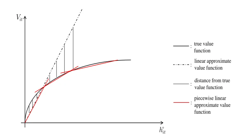
In this thesis, we study the portfolio selection problem with multiple risky assets, linear transaction costs and a risk measure in a multi-period setting. In particular, we formulate the multi-period portfolio selection problem as a dynamic program and to solve it we construct approximate dynamic programming (ADP) algorithms, where we include Conditional-Value-at-Risk (CVaR) as a measure of risk, for dif-ferent separable functional approximations of the value functions. We begin with the simple linear approximation which does not capture the nature of the portfolio selection problem since it ignores risk and leads to portfolios of only one asset. To improve it, we impose upper bound constraints on the holdings of the assets and we notice that we have more diversified portfolios. Then, we implement a piecewise linear approximation, for which we construct an update rule for the slopes of the ap-proximate value functions that preserves concavity as well as the number of slopes. Unlike the simple linear approximation, in the piecewise linear approximation we notice that risk affects the composition of the selected portfolios. Further, unlike the linear approximation with upper bounds, here wealth flows naturally from one asset to another leading to diversified portfolios without us needing to impose any additional constraints on how much we can hold in each asset. For comparison, we consider existing portfolio selection methods, both myopic ones such as the equally-weighted and a single-period portfolio models, and period ones such as multi-stage stochastic programming. We perform extensive simulations using real-world equity data to evaluate the performance of all methods and compare all methods to a market Index. Computational results show that the piecewise linear ADP algo-rithm significantly outperforms the other methods as well as the market and runs in reasonable computational times. Comparative results of all methods are provided and some interesting conclusions are drawn especially when it comes to comparing the piecewise linear ADP algorithms with multistage stochastic programming.
First and foremost, I would like to thank my supervisor, Dr Katerina Papadaki, for giving me the opportunity to undertake this PhD. Her enthusiasm about research and her expertise in the methods that were required by my topic have been invaluable in progressing with my doctoral work. Not to mention that, except for my thesis advisor, she has been a valuable friend of mine.
Furthermore, I am very grateful to my examiners, Professor Victor DeMiguel and Professor M. Grazia Speranza, for their constructive comments and feedback which gave me the opportunity to look at different aspects of the problem. With their help, the contributions of my thesis reflect much better and I am better able to communicate them.
Further, I owe a big thank you to my family, my father Nikiforos Karamanis, my mother Stavroula Karamani and my siblings Alexandra Karamani and Angelos Gkartzonikas to whom I am deeply indebted for their love and support all these years.
I would also like to thank my friends back in Greece, Christos, Evelyn, Sevi, Froso, Charis and Giorgos for standing by my side in good and bad times. I will never forget how impatient I have been towards the end of each term to go back to Greece, meet my friends and spend time with them.
Finally, I would like to thank the friends I made in London, Selvin, Ozlem, Camelia, Sumitra, Shweta, Nayat, Anastasia, Clodaugh, Nikos, and Sinan, for spending a good time with them in London and not only in London. I will al-ways remember our 3-4day trips to Paris, Ljubljana, Berlin, Lisbon, Amsterdam, Finland, Norway and many more other destinations. Together we had lots of fun!
Nomenclature 16
1 Introduction 18
1.1 Literature Review . . . 20
1.2 Thesis Outline . . . 23
I
Introduction to the Portfolio Selection Problem
25
2 Basic Concepts and Notation 26 2.1 Timing of Events and Dynamics . . . 262.2 Conditional-Value-at-Risk as a Measure of Risk . . . 29
2.3 Investor’s Objective . . . 32
2.4 Modeling Uncertainty . . . 34
II
Dynamic Programming Methods for the Portfolio
Selec-tion Problem
37
3 Dynamic Programming Formulation for the Portfolio Selection Prob-lem 38 3.1 Formulation . . . 383.2 Dynamic Programming and the Curses of Dimensionality . . . 44
3.3 CVaR and Dynamic Programming . . . 45
4 Approximate Dynamic Programming 46 4.1 Pre-decision and Post-decision State Variables . . . 47
4.2 CVaR Estimation Given a Sample of Losses . . . 52
4.3 General ADP Algorithm . . . 55
4.4 Gradient Information . . . 61
III
Portfolio Selection Methods used as Benchmarks
63
5 Stochastic Programming and the Equally-weighted Portfolio 64 5.1 Stochastic Programming . . . 645.1.1 The Single-period Portfolio as a Two-stage Stochastic Pro-gram . . . 66
5.1.2 The Multi-period Portfolio as a Multistage Stochastic Program 69 5.2 The Naive Equally-weighted Portfolio . . . 76
IV
Approximate Dynamic Programming Methods
78
6 Separable Linear Approximations 79 6.1 Linear Approximations for the Value Functions . . . 816.2 The Subproblem of LADP . . . 83
6.3 The Subproblem of LADP-UB . . . 92
6.4 Discussion . . . 105
6.5 Gradient Information . . . 106
7 Separable Piecewise Linear Approximation 110 7.1 Piecewise Linear Approximations for the Value Functions . . . 112
7.2 The Subproblem of PLADP . . . 115
7.2.1 Representing Piecewise Linear Functions in Optimization Problems . . . 115
7.2.2 Linear Programming Formulation of the Subproblem of PLADP121 7.2.3 Solution to the Subproblem of PLADP . . . 128
7.3 Update Rule for Value Functions . . . 141
V
Experimental Results, Conclusions and Future Research 151
8 Experimental Results 152 8.1 Performance Evaluation Design . . . 1528.1.1 Characteristic of Selected Portfolios and Convergence of Slopes . . . 155
8.2 Experimental Data and Design . . . 157 8.3 Numerical Results . . . 165
8.3.1 Characteristics of Selected Portfolios and Convergence of Slopes . . . 166 8.3.2 Performance Evaluation . . . 174 8.3.3 Expected Terminal Wealth and CVaR of the Different
Port-folio Policies . . . 192 8.3.4 Impact of Length of Planning Horizon . . . 194 8.3.5 Impact of Transaction Costs . . . 203
9 Conclusions and Future Research 209
9.1 Conclusions . . . 209 9.2 Future Research . . . 212
Appendices 214
A OGARCH in Scenario Generation 215
B Scenario Reduction and Scenario Tree Construction 217
C Derivation of Gradients for the LADP Methods 220
D Experimental Results: Scenario Reduction Parameters 228
4.1 Losses per scenarios . . . 55
4.2 Sorted losses . . . 55
6.1 Transformation coefficients . . . 105
6.2 Projection coefficients . . . 106
6.3 Observed slopes∆ ˜Vi(t−1)s in LADP . . . 108
6.4 Observed slopes∆ ˜Vs i(t−1)in LADP-UB . . . 109
7.1 Upper and lower bounds for variableszκ−andz+ κ . . . 119
7.2 Upper and lower bounds for variableswκ−andw+ κ . . . 120
7.3 Optimal decisions for the problem of Example9.2 . . . 131
7.4 Correspondence between the old variables and parameters and the new ones . . . 132
8.1 Dates of in-sample and out-of-sample data . . . 158
8.2 Average annual base rates and weekly interest rates in the four datasets159 8.3 Parameters and Values . . . 160
8.4 Characteristics of selected portfolios for the equally-weighted, the single-period and the multistage stochastic programming methods . 169 8.5 Characteristics of selected portfolios for the LADP methods . . . 170
8.6 Characteristics of selected portfolios for the PLADP methods . . . . 171
8.7 Out-of-sample terminal wealths . . . 177
8.8 In how many instances out of the 24a row method outperforms a column method . . . 178
8.9 Average out-of-sample terminal wealth for the market Index, the equally-weighted, the single-period and the multistage stochastic programming methods . . . 179
8.10 Average out-of-sample terminal wealth for the ADP methods . . . . 180
8.11 Average out-of-sample terminal wealths for different stepsize values 185 8.12 Computational times in seconds . . . 191 8.13 Up-Up, Up-Down: Expected Terminal Wealth of the Portfolio
Poli-cies of the PLADP methods and the equally-weighted strategies . . 192 8.14 Down-Up, Down-Down: Expected Terminal Wealth of the Portfolio
Policies of the PLADP methods and the equally-weighted strategies 193 8.15 Up-Up, Up-Down: CVaR of the Portfolio Policies of the PLADP
methods and the equally-weighted strategies . . . 193 8.16 Down-Up, Down-Down: CVaR of the Portfolio Policies of the PLADP
methods and the equally-weighted strategies . . . 194 8.17 Characteristics of selected portfolios for planning horizons of13,26
and52weeks . . . 196 8.18 Up-Up, Up-Down: Out-of-sample wealths at timest= 0,13,26,39
and 52 in the PLADP methods and the benchmarks for planning horizons of13,26and52weeks . . . 198 8.19 Down-Up, Down-Down: Out-of-sample wealths at timest= 0,13,26,39
and 52 in the PLADP methods and the benchmarks for planning horizons of13,26and52weeks . . . 199 8.20 In how many instances out of the 8a column PLADP method
out-performs a row method at timest = 13,26,39and52and for plan-ning horizons of13,26and52weeks . . . 200 8.21 Average out-of-sample wealths at times t = 0,13,26,39and52in
the PLADP methods and the benchmarks for planning horizons of
13,26and52weeks . . . 201 8.22 Average performance: In how many instances out of the2a column
PLADP method outperforms a row method at timest = 13,26,39
and52and for planning horizons of13,26and52weeks . . . 202 8.23 Up-Up and Up-Down datasets: Out-of-sample terminal wealths and
total transaction costs paid in the equally-weighted strategies for
θ= 0.2%and0.5% . . . 204 8.24 Down-Up and Down-Down datasets: Out-of-sample terminal wealths
and total transaction costs paid in the equally-weighted strategies for
θ= 0.2%and0.5% . . . 204 8.25 Percentage differences of the terminal wealths in the fixed-mix
8.26 Characteristics of selected portfolios, terminal wealth values and total transaction costs paid in PLADP methods forθ = 0.2%,0.5% . 206 8.27 In how many instances out of the8the PLADP methods outperform
the equally-weighted strategies and the market . . . 207
8.28 Average out-of-sample terminal wealths forθ = 0.2%and0.5% . . 207
D.1 Scenario reduction parameters in the Up-Up dataset . . . 229
D.2 Scenario reduction parameters in the Up-Down dataset . . . 230
D.3 Scenario reduction parameters in the Down-Up dataset . . . 231
1.1 System Structure . . . 20
2.1 Timing of events for the portfolio selection problem . . . 27
2.2 An illustration of VaRβ and CVaRβ on a discrete loss distribution . . 31
2.3 A concave utility function . . . 33
3.1 Decision Epochs and Periods for a MDP . . . 39
3.2 Timing of events in the portfolio selection problem . . . 41
3.3 Modeling time horizon: states and value functions . . . 43
4.1 Timing of events with pre- and post-decision state variables . . . 48
5.1 Sequence of events in a multistage stochastic program . . . 65
5.2 Timing of events and stages in the single-period portfolio problem . 67 5.3 Timing of events and stages in the multi-period portfolio selection problem . . . 71
5.4 A scenario tree with T + 1 stages, KT+1 nodes and KT+1 − KT scenarios . . . 72
5.5 A distribution of 100 scenarios on the left and its approximation on the right. . . 74
6.1 Linear approximate value function of assetiin periodt+ 1with an upper bound on its holdings . . . 80
6.2 Categories of assets and conditions . . . 86
6.3 Buying and selling slopes vs current holdings before allocation . . . 90
6.4 Step 1. Sell stock3and update cash . . . 91
6.5 Step 2. Buy stock1with cash . . . 91
6.6 Step 3. Sell stock2and buy stock1. . . 92
6.7 Buying and selling slopes vs current holdings before allocation . . . 103
6.8 Step 1. Sell stock2and stock3and update cash . . . 103
6.9 Step 2. Buy stock1with cash . . . 104
6.10 Step 3. Sell stock2and buy stock1. . . 104
7.1 Piecewise linear approximate value function of risky assetiin pe-riodt+ 1 . . . 111
7.2 Equivalent representations of a piecewise linear function with3slopes113 7.3 A piecewise linear curve with3slopes . . . 116
7.4 Maximizing the sum of two piecewise linear curves with 3 slopes each and one linear curve . . . 118
7.5 Decision variables for a piecewise linear value function with3slopes 122 7.6 Transition from original slopesuκ it to buying slopeskitκ and selling slopeslitκ . . . 127
7.7 Buying and selling slopes vs current holdings before allocation . . . 137
7.8 Step 1. Sell stock2and update cash . . . 138
7.9 Step 2. Buy stock1with cash . . . 138
7.10 Step 3a. Sell stock 3 and buy stock 1 . . . 139
7.11 Step 3b. Sell stock 2 and buy stock 1 . . . 139
7.12 Update rule for problems with discrete state space and a violation in the monotonicity of the slopes from the left . . . 145
7.13 Update rule for problems with continuous state space and a violation in the monotonicity of the slopes from the left . . . 147
7.14 Correction rule for problems with continuous state space and a vio-lation in the number of slopes . . . 148
8.1 FTSE100 price Index from 03/01/1995 until 03/01/2005 and the four market periods . . . 158
8.2 Different rates of convergence for stepsize ruleαs = b (b−1)+s . . . . 162
8.3 Slope versus iteration for asseti= 3at timet = 30and forγ = 0.8 in the Up-Up dataset in the LADP method . . . 172
8.4 Slope versus iteration for asseti= 3at timet = 30and forγ = 0.8 in the Up-Up dataset in the LADP-UB method . . . 172
8.5 Slopes versus iteration for asseti= 3at timet = 30and forγ = 0.8 in the Up-Up dataset in the PLADP method withm= 3slopes . . . 173
8.9 Average out-of-sample cumulative wealth against time forγ = 0.6 . 182 8.10 Average out-of-sample cumulative wealth against time forγ = 0.8 . 182
8.11 Average out-of-sample cumulative wealth against time forγ = 1 . . 183
8.12 Average performance for different stepsizes: γ = 0 . . . 186
8.13 Average performance for different stepsizes: γ = 0.2 . . . 186
8.14 Average performance for different stepsizes: γ = 0.4 . . . 187
8.15 Average performance for different stepsizes: γ = 0.6 . . . 187
8.16 Average performance for different stepsizes: γ = 0.8 . . . 188
8.17 Average performance for different stepsizes: γ = 1 . . . 188
8.18 Average out-of-sample cumulative wealth forγ = 0.2and planning horizons of13,26and52weeks . . . 202
8.19 Average out-of-sample cumulative wealth forγ = 0.6and planning horizons of13,26and52weeks . . . 203
8.20 Average out-of-sample cumulative wealth forγ = 0.2andθ = 0.2% and0.5%. . . 207
8.21 Average out-of-sample cumulative wealth forγ = 0.6andθ = 0.2% and0.5%. . . 208
E.1 Out-of-sample cumulative wealth against time: Up-Up,γ = 0 . . . . 233
E.2 Out-of-sample cumulative wealth against time: Up-Up,γ = 0.2. . . 234
E.3 Out-of-sample cumulative wealth against time: Up-Up,γ = 0.4. . . 234
E.4 Out-of-sample cumulative wealth against time: Up-Up,γ = 0.6. . . 235
E.5 Out-of-sample cumulative wealth against time: Up-Up,γ = 0.8. . . 235
E.6 Out-of-sample cumulative wealth against time: Up-Up,γ = 1 . . . . 236
E.7 Out-of-sample cumulative wealth against time: Up-Down,γ = 0 . . 237
E.8 Out-of-sample cumulative wealth against time: Up-Down,γ = 0.2 . 237 E.9 Out-of-sample cumulative wealth against time: Up-Down,γ = 0.4 . 238 E.10 Out-of-sample cumulative wealth against time: Up-Down,γ = 0.6 . 238 E.11 Out-of-sample cumulative wealth against time: Up-Down,γ = 0.8 . 239 E.12 Out-of-sample cumulative wealth against time: Up-Down,γ = 1 . . 239
E.13 Out-of-sample cumulative wealth against time: Down-Up,γ = 0 . . 240
4.1 General ADP Algorithm . . . 59 6.1 Allocation Algorithm for Linear Approximation . . . 87 6.2 Allocation Algorithm for Linear Approximation with Strict Control
of Flows . . . 96 7.1 Allocation Algorithm for Piecewise Linear Approximation . . . 135 7.2 Slopes Update and Correction Routine . . . 149
N Set of risky assets
T Set of discrete points in time horizon
T End of time horizon
xit How much we buy from risky assetiat timet
xt Vector of buying variables at timet
yit How much we sell from risky assetiat timet
yt Vector of selling variables at timet hit Pre-decision holdings of assetiat timet
ht Vector of pre-decision holdings at timet
h+it Post-decision holdings of assetiat timet
h+t Vector of post-decision holdings at timet Rit Rate of return of risky assetiat timet
Rt Vector of rates of returns of risky assets at timet
Vit Value function of assetiat timet
uit Slope of assetiin value functionVitat timet
υT Total wealth at timeT
γ Risk importance parameter
θ Proportional transaction costs per (monetary) unit of asset traded
s Scenario
n Node
pn Probability of noden
K Set of nodes on a scenario tree
Kt Set of nodes at stagetof a scenario tree
C(n) Set of children nodes of nodenon a scenario tree
kn Predecessor node of nodenon a scenario tree VaR Value-at-Risk
CVaR Conditional-Value-at-Risk SP Stochastic Programming
MSP Multistage Stochastic Programming DP Dynamic Programming
ADP Approximate Dynamic Programming
Introduction
The fundamental contribution of this thesis is the development of approximate dy-namic programming (ADP) algorithms that solve the portfolio selection problem
over a long-termplanning horizon. Conditional-Value-at-Risk (CVaR) is used as a
measure of riskandtransaction costsare taken proportional to the trading amounts. Specifically, in this study we formulate the portfolio selection problem as a
dynamic program, which due to the high-dimensional state, outcome and action spaces becomes quickly computationally intractable. To solve it, we use approx-imate dynamic programming methods, which provide a time decomposition and approximation framework that breaks long-term horizon problems into a group of smaller problems that can be solved using mathematical programming methods.
Thecontributionsof this thesis can be summarized as follows:
1. To our knowledge, so far ADP methods have been applied mainly to one-dimensional financial problems without risk. Here, we expand this by apply-ing ADP methods to a multi-dimensional portfolio selection problem with a widely used measure of risk and transaction costs.
2. We introduce a novel piecewise linear ADP scheme that can handle high-dimensional problems. By controlling the number of slopes in the piecewise linear value function approximations and allowing the value of the slopes and the slope intervals to be adaptively estimated, we end up with a scheme that runs in reasonable times and performs extremely well against the competing methods.
3. We provide a novel comparative analysis between a large range of portfolio selection methods, where we compare various ADP algorithms of increasing
complexity against:
(a) Myopic portfolio selection methods: A single-period and the equally-weighted portfolio methods, where decisions on portfolio composition at any point in time ignore their impact in the future.
(b) Multi-period portfolio selection methods: Multistage stochastic pro-gramming (MSP), where the investor accounts for both the short-term and the long-term effects of the investment strategies. In a discrete time setting, this is achieved by considering an investmentplanning horizon, where the investor has to take temporal decisions in order to achieve a goal at some date in the future.
A comparison against amarket Indexis included.
4. In the ADP methods, we need to solve a large number of linear programs the complexity of which varies depending on the assumed value function ap-proximations and increases significantly for the piecewise linear approxima-tions. Solving these linear programs with mathematical programming meth-ods takes a long time. Here, we construct greedy algorithms for all approxi-mation schemes that solve our linear programs much faster and we prove that the solutions we get from these algorithms are optimal.
To evaluate the proposed approximate dynamic programming algorithms, we use real-life equity data from the London Stock Exchange and we divide into the following two parts: the in-sample data which we use to generate scenario paths and the out-of-sample data which we use to test the methods. For robustness, we have considered all combinations of the market going up or down in the in-sample and out-of-sample data.
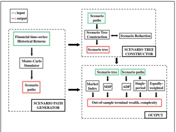
tree using scenario reduction and scenario tree construction methods. The gener-ated scenario tree serves in turn as an input for the multistage stochastic program-ming method. For each method we compute the out-of-sample terminal wealth (see output part in figure 1.1) which is our performance measure and all methods are compared in terms of performance and complexity.
: input : output
SCENARIO PATH GENERATOR Financial time-series:
Historical Returns Monte-Carlo
Simulator Scenario
paths
Scenario paths Scenario Tree
Construction Scenario Reduction Scenario tree SCENARIO TREE
CONSTRUCTOR
MSP ADP
Out-of-sample terminal wealth, complexity Scenario tree Scenario paths
Single- period Market
Index
[image:20.595.136.489.211.475.2]OUTPUT Equally- weighted
Figure 1.1: System Structure
1.1
Literature Review
In this section, we briefly describe the current state of the art in the era of portfolio optimization. More literature regarding the methods used in this study is provided in the respective chapters.
maxi-mum expected return for any given level of risk (variance). Following the work of Markowitz, Tobin showed in 1958 (see [78]) that including a risk-free asset in the portfolio of assets the efficient frontier changes from a hyperbola to a straight line, which led to the so called CAPM model (see [75]).
Despite its theoretical reputation, researchers very early identified that with the available mathematical tools back then the computational burden in solving the port-folio model of Markowitz increased substantially with the number of assets since constructing large-scale portfolios requires solving large-scale quadratic optimiza-tion problems (due to variance) with dense covariance matrices. Researchers at-tempted to alleviate this difficulty from the early years of the history of the modern portfolio theory by introducing factors that drive the stock prices (see for example the index models in [63] and [73]) or by introducing approximation schemes, where linear programming plays a central role (see for example [74] and [76]). The im-portance of linear programming in financial applications has grown further by the need to include binary variables that help us model other realistic features, such as transaction costs (see for example [39]). Interest in how transaction costs can af-fect investors’ decisions on portfolio composition goes back to Samuelson [71] and Constantinides [14].
Ever since Markowitz, there have been several attempts to formulate the single-period portfolio optimization problem as a linear program. All these attempts have focused on using risk measures, which for discrete approximations of the distri-butions of returns lead to Linear Programming computable models. Yitzhaki [84] used the Gini’s Mean Difference (GMD) as a measure of risk and proposed the so called GMD model. Konno and Yamazaki [47] used the Mean Absolute Deviation (MAD) as a measure of risk and proposed and analyzed the so called MAD model. Another group of risk measures includes the so called downside risk measures. The importance of downside risk measures lies in the behavior of rational investors, who are more interested in the underperformance than the overperformance of portfolios. Markowitz [55] recognized the importance of downside risk measures and proposed the use of semivariance as a measure of risk. For a more comprehensive review of the various risk measures and the single-period portfolio models that exist in the literature, we refer the reader to [53] and references therein.
possible losses. However, VaR has received a lot of criticism due to lacking sub-additivity, which means that the risk of a portfolio of assets may be greater than the sum of the individual risks of the assets. This makes VaR a non-coherent risk mea-sure in the Artzner et al. sense [3]. A modified version of VaR, called Conditional-Value-at-Risk (CVaR), was introduced in 2000 by Rockafellar and Uryasev (see [70]) and has recently become very popular in the era of financial optimization due to its properties (for applications see for example [2], [38] and [48]). CVaR is a coherent risk measure that accounts for losses which occur in the tails of the distri-butions of returns and for discrete approximations of the distridistri-butions of returns it can be approximated with a linear program, and thus can be easily incorporated in optimization procedures.
Despite the large body of literature in single-period portfolio models, the latter have received a lot of criticism mainly due to their inability to take advantage of (ex-pected) future information when rebalancing the portfolios. Also, they have been found to be inadequate in modeling correctly situations where long-term investors face liabilities and goals at specific dates in the future. To circumvent these ineffi-ciencies, several authors have attempted to model the portfolio selection problem in a multi-period setting. In general, for long term investors multi-period models will perform better than the single-period ones. For a discussion about the advantages of using multi-period models versus single-period ones see [58]. Due to multi-period models being more complex than the single-period ones, in the early years of the modern portfolio theory some authors proposed solving the large-scale multi-period portfolio selection problem as a sequence of single-period portfolio models (see for example [30], [42], [56] and [57]).
1.2
Thesis Outline
The thesis is structured as follows:
• Part I: Introduction to the Portfolio Selection Problem. In this part, we introduce the reader to the portfolio selection problem. Specifically, in chap-ter 2 we provide the notation used throughout this study, derive the rela-tionships between the variables in the portfolio selection problem, introduce Conditional-Value-at-Risk as a measure of risk and describe how the multi-variate process of random returns can be modeled using scenario generation methods.
• Part II: Dynamic Programming Methods for the Portfolio Selection Prob-lem. In this part, we formulate the portfolio selection problem as a dynamic program without a measure of risk in chapter 3 and, due to the curses of dimensionality, to solve it in chapter 4 we construct approximate dynamic programming algorithms where we include Conditional-Value-at-Risk as a measure of risk.
• Part III: Portfolio Selection Methods used as Benchmarks.In this part, we describe the portfolio selection methods that we use as benchmarks in order to compare with the approximate dynamic programming methods. Specifically, in chapter5we use stochastic programming methods to formulate and solve the single-period as well as the multi-period portfolio selection problems and we provide the linear programming formulation of the naive equally-weighted portfolio model.
• Part IV: Approximate Dynamic Programming Methods. In this part, we discuss approximate dynamic programming methods. Specifically, we first implement separable linear approximations for the unknown value functions in the dynamic programming formulation of the portfolio selection problem in chapter6and then we improve them by implementing a separable piecewise linear approximation in chapter7.
Introduction to the Portfolio
Selection Problem
Basic Concepts and Notation
In this chapter, we summarize the basic concepts in the portfolio selection problem and the notation adopted throughout this study. Specifically, in section 2.1 we define the variables in the portfolio selection problem and derive the relationships between them. Then, in section 2.2 we introduce Conditional-Value-at-Risk as a measure of risk and write it as an optimization problem. Next, in section 2.3 we discuss the utility function of a risk-averse investor and present our objective. Finally, we conclude this chapter with section 2.4, where we discuss how the uncertainty that is introduced by the random returns can be modeled using scenario generation meth-ods.
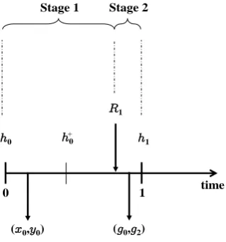
2.1
Timing of Events and Dynamics
Figure 2.1 shows how transactions evolve in time. Time is divided into equal length sub-periods called slots, such that period t corresponds to the time slot between timet−1and timet. We let thehorizonbe the set of all discrete points in time and we denote asT = {0,1, . . . , T}, whereT is theend of the time horizon. Suppose we have a portfolio that comprises ofN risky assets, such thatN is the set of risky assets, i.e. N ={1,2, . . . , N}, and a risk-free one. Without loss of generality, we assume that asset 0 is the risk-free asset and is simply a bank account that pays a known constant interest rate at the end of every time period. We denote the rate of return of the risk-free asset in periodtwithR0t. For simplicity, from this point on we will use termcashto refer to the risk-free asset.
Looking at Figure 2.1, in periodt+1events evolve in the following sequence: At timetthedecision maker, i.e. the investor, owns holdingsht= (h0t, h1t, . . . , hN t),
wherehit is the amount of wealth (in monetary units) in asset categoryiat timet, and takes actions(xt,yt), wherext= (x1t, x2t, . . . , xN t)andyt= (y1t, y2t, . . . , yN t) are respectively vectors of how much the investor buys and sells (in monetary units) from every risky asset at the beginning of periodt+1. Every buying/selling decision
xit/yit increases/decreases the amount of holdings in asset i at time t by the same amount. That is, every pair of decisions(xit, yit)change the amount of holdings in assetitoh+it =hit+xit−yit.
Buying and selling cause transaction costs, which in this study are assumed to be proportional to the trading amount, independent of the asset category and time, and are denoted with θ. Specifically, buying one unit of asset i requires (1 +θ)
units of cash, while selling one unit of asset i increases cash by (1 −θ) units. Therefore, decisions(xt,yt)change the amount of cash fromh0tat timettoh+0t =
h0t− (1 +θ)
PN
i=1xit + (1− θ)
PN
i=1yit. Note that due to transaction costs it is suboptimal to simultaneously buy and sell the same asset. We will see later on that we need not make this assumption as it is directly inferred by the optimization problems that we solve in every time period.
After taking decisions(xt,yt), which as explained above change the amount of holdings toh+t = h+0t, h+1t, . . . , h+N t, the random return vector Rt+1 gets realized, where Rt+1 = R1(t+1), R2(t+1), . . . , RN(t+1)
and Ri(t+1) is the rate of return of risky asset i at the end of period t+ 1. Due to the returns, holdings at time t + 1 become ht+1 = h0(t+1), h1(t+1), . . . , hN(t+1)
, where hi(t+1) = Rith+it. In the above modeling context, we assume that holdingsh0are known to the investor with certainty.
time
h0
…
h1 h2 hT−1 hT
(x0,y0)
R1 R2 RT
0 1 2 T−1 T
h0 +
h1 +
hT−1 +
period 1
…
period T period 2
(x1,y1) (xT−1,yT−1)
Figure 2.1: Timing of events for the portfolio selection problem
before decisions (xt,yt), are called the pre-decision holdings and, as we will see in chapter 3, these become our state variables in the optimal dynamic programming formulation of the portfolio selection problem. Variables h+t are sequenced right after decisions(xt,yt), are called thepost-decisionholdings and, as we will see in chapter 4, these become our new state variables in approximate dynamic program-ming. Further, variablesh+t are used in the two-stage stochastic programming for-mulation of the single-period portfolio selection problem, the multistage stochastic programming formulation of the multi-period portfolio selection problem and the equally-weighted portfolio model in chapter 5.
We are now ready to write the relationships between the variables in the portfolio selection problem.
Considering the above and looking at Figure 2.1, we obtain the relationships between the pre-decision variables:
hi(t+1) =Ri(t+1)(hit+xit−yit), i∈ N
h0(t+1) =R0(t+1)
"
h0t−(1 +θ) N
X
i=1
xit+ (1−θ) N
X
i=1
yit
#
(2.1)
where note that first decisions are taken and then returns are realized, and the post-decision variables:
h+i0 =hi0+xi0−yi0, i∈ N
h+00=h00−(1 +θ) N
X
i=1
xi0+ (1−θ) N
X
i=1
yi0
h+it =Rith+i(t−1)+xit−yit, i∈ N, t = 1, . . . , T −1
h+0t=R0th+0(t−1)−(1 +θ) N
X
i=1
xit+ (1−θ) N
X
i=1
yit, t= 1, . . . , T −1
(2.2)
where note that first returns are realized and then decisions are taken.
Further, the pre- and the post-decision variables have the following relationship:
have:
υT =
N
X
i=0
hiT = N
X
i=0
RiTh+i(T−1) (2.4)
In this study, we do not consider either shortselling of assets or borrowing of cash. Instead, we assume non-negativity of the pre- and post-decision variables, as well as of the amounts traded (either bought or sold) in every time period. Non-negativity can be expressed by the following set of inequalities:
hit ≥0, i∈ N ∪ {0}, t= 1, . . . , T
h+it ≥0, i∈ N ∪ {0}, t= 0, . . . , T −1
xit≥0, i∈ N, t= 0, . . . , T −1
yit ≥0, i∈ N, t= 0, . . . , T −1
(2.5)
where, as we will explain later on, due to transaction costsxitandyit are never both positive.
2.2
Conditional-Value-at-Risk as a Measure of Risk
One essential aspect in portfolio optimization is risk measurement. In this study, we useConditional-Value-at-Risk(CVaR), also known asmean excess lossormean shortfallortail-VaR, as a measure of risk. The reason why we selected in this study CVaR as the risk measure is because of the properties it exhibits. Specifically, CVaR is a coherent downside risk measure which accounts for possible extreme losses that occur in the tails of loss distributions. Moreover, for a discrete set of scenarios it can be approximated with a linear program, thus allowing us to incorporate it easily in optimization procedures. In the discussion that follows, we briefly state the definition of CVaR in line with [70], its properties and its representation as a linear program for a discrete approximation of the random input.
Definition
Letf(X, Y)be the loss associated with decision vectorX ∈ X and random vector
Ψ(X, g0) =
Z
f(X,Y)≤g0
p(Y)dY (2.6)
For a specified probability level β ∈ (0,1)and the losses associated with de-cision vectorX, the values of Value-at-Risk (VaRβ) and Conditional-Value-at-Risk (CVaRβ) are denoted respectively withφβ(X)andχβ(X). These are given by:
φβ(X) = min{g0 ∈R: Ψ(X, g0)≥β}, (2.7)
χβ(X) =
1
1−β
Z
f(X,Y)≥φβ(X)
f(X, Y)p(Y)dY (2.8)
The key to expressing CVaRβ as a linear minimization problem is the following function:
Fβ(X, g0) = g0+
1 1−β
Z
Y∈Y
[f(X, Y)−g0] +
p(Y)dY (2.9)
where[k]+ =k ifk >0and[k]+= 0ifk≤0.
In optimization problems, we are interested in minimizing CVaRβ over allX ∈ X. According to theorem2in [70], minimizingχβ(X)over allX ∈ X is equivalent to minimizingFβ(X, g0)over all(X, g0)∈ X ×R, i.e. we have:
min
X∈Xχβ(X) =(X,gmin0)∈X ×R
1-β
VaRβ max loss
loss
fr
equency
CVaRβ
Figure 2.2: An illustration of VaRβand CVaRβon a discrete loss distribution
Properties of CVaR
With respect to loss functionf(·), which is a random variable, CVaR satisfies the following properties:
1. CVaR istranslation-equivariant. That is,
CVaR(f +c) =CVaR(f) +c (2.11)
2. CVaR ispositively-homogeneous. That is,
CVaR(cf) = cCVaR(f), (2.12)
ifc > 0.
3. CVaR isconvex. That is, for two arbitrary random lossesf1 andf2 and0 <
λ <1we have:
CVaR(λf1 + (1−λ)f2)≤λCVaR(f1) + (1−λ)CVaR(f2) (2.13)
4. CVaR is monotone. That is, for any arbitrary random losses f1 and f2 if
f1 ≤f2, then we have:
For the proofs of the above properties, we refer the reader to [82]. In the Artzner, Delbaen, Eber and Heath sense [3], a risk measure that exhibits properties (2.11)-(2.14) is calledcoherent.
Polyhedral Representation of CVaR
We are now ready to derive thepolyhedralrepresentation of CVaR.
Suppose we sample Sscenarios from the distribution of random variable Y. If Sis the set containing all scenarios, i.e.S ={1,2, . . . , S}, andpsis the probability associated with scenarios, then the integral in (2.9) can be approximated by:
˜
Fβ(X, g0) =g0+
1
1−β
S
X
s=1
ps[f(X, Ys)−g0] +
(2.15)
If we replace in (2.15) every[f(X, Ys)−g0] +
with auxiliary variablegs2, we can approximate CVaR with the optimal value of the following linear program:
min (X,g0,g2s)∈
X ×R×R+
g0+
1 (1−β)
S
X
s=1
psgs2
s.t. g2s ≥ −g0+f(X, Ys), s∈ S
g0 free, gs2 ≥0, s∈ S
(2.16)
Using problem (2.16), later on in chapter4we define CVaR for the multi-period portfolio selection problem and we adapt it for each other method in the respective chapters.
2.3
Investor’s Objective
The goal of the investor is usually expressed as the expected utility of some function of terminal wealth:
maxE[U(υT)] (2.17)
An investor with a concave utility function is said to be risk-averse. For a more detailed discussion about utility theory and risk-aversion, we refer the reader to chapter 9 of [52].
U
υT
Figure 2.3: A concave utility function
In this study, we consider a mean-risk objective function, according to which the investor aims at co-optimizing a weighted average of the expected terminal wealth and CVaR:
maxγE
υT −(1−γ)CVaR(υT) (2.18) where parameterγ measures how important is risk in the objective, takes values in the range[0,1], and will be called therisk importance parameter. In problems with long horizons, in order to account for the time value of money, we usually see a discount factor outside the expectation of objective (2.18). However, in the portfolio selection problem the time value of money is accounted by the asset returns and thus we disregard it.
Note that objective (2.18) is a concave function ofυT due to CVaR being convex with respect toυT (this follows from property 2.13, where the loss function is now given by−υT plus a constant). To understand how the risk attitude of the investor is affected by the value of parameterγ, we can form ratio 1−γγ , which simply tells us how important CVaR is as compared to expected terminal wealth, takes values in the range[0,∞), and is usually called therisk aversion coefficient. If 1−γγ = 0, then the investor is infinitely risk-taking, while if 1−γγ → ∞then the investor is infinitely risk-averse.
effi-cient frontier of terminal wealth, every point of which represents the best possible expected terminal wealth for a given level of CVaR. The efficient frontier is a hy-perbola, reflecting the investor’s risk-averse attitude (he expects to earn less and less the more he is exposed to higher losses).
2.4
Modeling Uncertainty
The random returns of the risky assets in equations (2.1)-(2.4) introduce uncertainty that can be described by the multivariate stochastic process of random returns and is usually represented in stochastic optimization with probability spaces.
For the stochastic process of random returns we define probability space(Ω,F,P), where:
1. Ωis the continuous sample space consisting of all realizationsω, whereω = (R1,R2, . . . ,RT)is a particular instance of the complete set of returns and is usually referred to as ascenario.
2. F is theσ-algebra onΩ, i.e. a non-empty collection of subsets ofΩthat in-cludesΩ. In chapter 5, we will needFt, which is theσ-algebra on(R1,R2, . . .
,Rt), i.e.Ftis a collection of all events determined by information available up to timet. For setFt, we haveFt ⊂ Ft+1 and is called afiltration. When a policy depends on information available up to time t, then this policy is callednon-anticipativeand for the respective decisions we say that they are Ft-measurable.
3. P is a function that maps any subset ofΩinto the unit interval[0,1], such that P(Ω) = 1.
For a further discussion on probability spaces and measures see [9] and [72]. When formulating stochastic problems, probability space(Ω,F,P)is assumed to be known. In order to obtain a finite and discrete probability space that results in a tractable stochastic model, we need to generate a discrete approximation of the probability space using scenario generation methods. In the literature, most sce-nario generation methods have been developed for multistage stochastic program-ming and are based upon:
2. the construction of ascenario tree.
For a comprehensive survey of the different models that have been used in the literature to generate data trajectory paths and the different scenario tree generation methods see [24] (other examples can be found in [25] and [41]).
Among the different models that have been used to generate data trajectories, econometric models have gained particular attention and have been used extensively to model and forecast the conditional variance, else known as volatility. A typi-cal feature of financial time series isvolatility clustering, according to which large volatilities tend to be followed by large volatilities, while small volatilities tend to be followed by small volatilities. Any changes from large volatilities to small ones and vice versa occur randomly without exhibiting any systematic pattern. Further, plotting the sample autocorrelation function (ACF) of the squared returns, one no-tices that squared returns exhibit strong positive autocorrelation, which provides more evidence of volatility clustering. Observations of this type led to the intro-duction of the so-called Generalized Autoregressive Conditional Heteroskedasticity (GARCH) models (see [11] and [28]).
Univariate GARCH models have been extended to a multivariate setting in order to study the co-movements of the assets’ volatilities by modeling and forecasting a positive definite conditional covariance matrix. The proposed models are known as multivariate GARCH models (MGARCH) (see [4] for a comprehensive survey). However, direct generalizations of the univariate GARCH models lead to intractable models as the dimensionality of the stochastic process becomes larger and larger and this is due to the large number of parameters that need to be estimated (this is often referred to as thecurse of dimensionality). This is the reason why these models have not been used in multivariate time series of more than three or four dimensions.
To circumvent the curse of dimensionality and obtain tractable models, addi-tional structures are imposed in order to reduce the dimensionality of the stochastic processes. One, very popular for its simplicity, method suggests the generation of the covariance matrix through an orthogonal factorization of the assets using prin-cipal component analysis. This class of models are known as Orthogonal GARCH (OGARCH) models (see [1]) and in comparative studies against other MGARCH models they have exhibited exceptional forecasting ability (see for example [12] and [29]).
Dynamic Programming Methods for
the Portfolio Selection Problem
Dynamic Programming Formulation
for the Portfolio Selection Problem
In this chapter, we formulate the multi-period portfolio selection problem as a dy-namic program (DP) without using a risk measure. As we will explain later in the chapter, we cannot include a risk measure such as CVaR in the dynamic program-ming formulation because then the problem does not decompose in time. Later on, in chapter 4, we incorporate CVaR as a risk measure in our approximation algo-rithms.
This chapter is structured as follows: In section 3.1, we define the basic elements of the portfolio selection problem as a markov decision process (MDP), state the objective function and derive the optimality equations. Then, in section 3.2, we discuss the curses of dimensionality, where we explain why we cannot solve the dynamic program defined in section 3.1 with the available dynamic programming algorithms and as a result we resort toapproximate dynamic programming. Finally, we conclude with section 3.3 where we explain why we cannot include CVaR in the optimal dynamic programming formulation.
More details regarding dynamic programming methods can be found in [7] and [69].
3.1
Formulation
In line with [69], we begin with defining the five elements of a markov decision process, i.e. decision epochs, states, actions, transition probabilities and rewards, which are related as follows: At each decision epoch the system occupies a state.
The decision maker observes the current state of the system and selects an action from a set of allowable actions. As a result of choosing an action in the current state of the system, the decision maker receives some reward and the system transits to some other state determined by some probability distribution. Note that in some cases the reward might also depend on the probability distribution. Given that we currently occupy a certain state, any future state/decision/outcome is independent of how we reached the current state, which is known as themarkov property.
Decision Epochs and Periods
Adecision epochrefers to a discrete point in time. We let thehorizonbe the set of all the decision epochs and we denote it with T = {0,1, . . . , T}. We divide time intoperiods, such that periodtcorresponds to the time slot between decision epoch
t−1and decision epoch t. Theend of the time horizon refers to the last decision epoch, which we denote withT. Figure 3.1 shows decision epochs and periods for a MDP.
time Decision
Epoch 0
Decision Epoch
1
Decision Epoch
2
Decision Epoch
T-1
Decision Epoch
T
Period 1 Period 2 Period T
…
Figure 3.1: Decision Epochs and Periods for a MDP
The State of the System and the Stochastic Process
Suppose setsHiandRi are respectively subsets ofR+andR+\ {0}.We let the state of the systembe described by vector ht = (h0t, h1t, . . . , hN t), whereht∈ H=H0× H1× · · · HN, andhitis the amount of holdings (in monetary units) of asset categoryiat timetand takes values inHi.
An important aspect of our problem is the arrival of exogenous information, which, as explained in section 2.4, is described by the stochastic process of random returns. A realization of the stochastic process at time t is described by vector
of return of assetiat timetand takes values inRi. Recall that the returns of cash,
R0t, are assumed to be known with certainty for everyt.
Policies and Decision Rules
The decisions associated with the portfolio selection problem are to determine how much thedecision maker, i.e. the investor, buys and sells from every asset in every time period. Let xt = (x1t, x2t, . . . , xN t) and yt = (y1t, y2t, . . . , yN t) be respec-tively the buying and selling decision vectors, withxitandyitrepresenting respec-tively how much the investor buys and sells from risky assetiat timet. We assume that(xt,yt)∈ At, whereAtis the set of constraints that determine all the feasible decisions for all assets at timet.
We define a decision rule to be a function that takes as input the current state variables and returns a vector of feasible decisions:
Dt(ht) = (xt,yt) (3.1)
We define apolicyπ to be a set of decision rules over all periods:
π = D0π(h0), D1π(h1), . . . , DπT−1(hT−1)
, π∈Π, (3.2) whereΠis the set of all feasible policies.
If we combine the equations in (2.1) with the non-negativity inequalities in (2.5), we obtain action spaceAt for everyt = 0,1, . . . , T −1, which is the set of values
(xt,yt)that satisfy the following constraints:
−xit+yit ≤hit, i∈ N, (3.3)
(1 +θ)
N
X
i=1
xit−(1−θ) N
X
i=1
yit ≤h0t, (3.4)
xit, yit≥0, i∈ N, (3.5) where constraint (3.3) ensures non-negativity of the holdings of the risky assets, constraint (3.4) ensures non-negativity of cash and will be called the budget con-straint, and finally constraint (3.5) ensures non-negativity of the buying and selling decisions of the risky assets.
At={(xt,yt) : (3.3)−(3.5)hold}, t= 0,1, . . . , T −1 (3.6)
Information Process
Looking at Figure 3.2, we notice that in every time period the events of the multi-period portfolio selection problem are disclosed in the following order: state vari-ables (i.e. holdings) at the beginning of the period, decisions, random returns and state variables (i.e. holdings) at the end of the period.
time …
0 1 2 T-1 T
period 1
…
period T period 2
h0 h1 h2 hT−1 hT
(x0,y0)
R1 R2 RT
(x1,y1) (xT−1,yT−1)
Figure 3.2: Timing of events in the portfolio selection problem
Given the above modeling of the time horizon, for every period t we let the
history of the process, else known as the information process, consist of all the information known to the system up to and including period t. The decisions and the states of the system represent the endogenous information, while the random returns represent the exogenousinformation. The history of the process for some policyπ ∈Πup to timetcan then be described as follows:
Ht= h0, Dπ0(h0),R1,h1, . . . ,ht−1, Dt−1π (ht−1),Rt,ht
(3.7)
Transition Functions
Assuming that at timet−1the state of the system is ht−1 and we take decisions
xt−1,yt−1
hit =Rit
hi(t−1)+xi(t−1)−yi(t−1)
, i∈ N
h0t=R0t
"
h0(t−1)−(1 +θ) N
X
i=1
xi(t−1)+ (1−θ) N
X
i=1
yi(t−1)
#
(3.8)
The above equations show how we transit from a current state to the next feasible state and are called thetransition functions.
Rewards and Objective
The objective of the investor is to find the best policy that maximizes expected terminal wealth which from (2.4) is a function of state variableshiT and is given by
υT =PN
i=0hiT. We define the following function:
Ctπ = (
0, if t∈ T \ {0, T}
PN
i=0hπiT, if t=T
to be therewardachieved at timetgiven that we follow policyπ, wherehπ iT is the amount of terminal holdings in assetiwhen policyπis followed.
Given the above definition, the objective of the investor can now be expressed as follows:
max
π∈Π E
( T
X
t=1
Ctπ
)
(3.9)
Note that in optimization problem (3.9) we do not use a discount factor, since the opportunity cost of cash held into assets is directly calculated by the returns of the assets.
Optimality Equations
In most problems, optimization problem (3.9) is computationally intractable. To reduce complexity, we formulate it as a dynamic program using recursive equations. We introduce thevalue functionVt(ht), which represents the value of being in state
time
h0
…
h1 h2 hT−1 hT
(x0,y0)
R1 R2 RT
0 1 2 T−1 T
V0(h0) V1(h1) V2(h2) VT−1(hT−1) VT(hT)
(x1,y1) (xT−1,yT−1)
Figure 3.3: Modeling time horizon: states and value functions
The quantityVt(ht)gives us the total optimal reward from timetuntil the end of the time horizon, given that at timetwe are in stateht, and is given by:
Vt(ht) = max (xt,yt)∈At
ERt+1{Vt+1(ht+1)|ht}, t = 0,1, . . . , T −1
VT(hT) = N
X
i=0
hiT
(3.10)
The recursive equations in (3.10) give us the relationship between Vt(ht)and
Vt+1(ht+1) for t = 0,1, . . . , T − 1 and are known as the Bellman’s optimality
equations. Note that inside the expectation of the optimality equationshtis constant butht+1is a function ofRt+1which is a random variable.
Normally we would expect to see a reward function and a discount factor in the optimality equations of (3.10). However, as explained earlier, here all the one-period rewards are zero and the investor receives the total reward only once at the end. Further, the time value of money is accounted by the returns and we do not need to use a discount factor.
For a discrete approximation of the joint distribution of the random returns and a discrete approximation of the states, we can replace the expectation in (3.10) with transition probabilities and write the optimality equations as follows:
Vt(ht) = max (xt,yt)∈At
X
ht+1∈H
p(ht+1 |ht,xt,yt)Vt+1(ht+1), t= 0,1, . . . , T −1
VT(hT) = N
X
i=0
hiT
(3.11) where p ht|ht−1,xt−1,yt−1
to state ht given that we choose action xt−1,yt−1
when we are in state ht−1 at timet−1.
3.2
Dynamic Programming and the Curses of
Dimen-sionality
In classical dynamic programming, authors solvefinite horizon problems, such as the one under study, using backward dynamic programming (see [65] and [69]) which assumes that we have discrete action, outcome and state spaces. Solving a dynamic program with backward dynamic programming is straightforward: At the end of the time horizon, we compute for each terminal state the terminal value func-tion. Then, we recursively step back one time period computing the value function for all states using the optimality equations. In this manner, in the end we will have computed the value function at time0which is the optimal value of problem (3.9).
In our problem, however, we have continuous action/outcome/state spaces. Even if we discretize actions and states to the nearest pound and also discretize returns the problem is still hard to solve due to the threecurses of dimensionality(see [65]). The first one comes from the state space which in our problem grows intractably large because the state of the system is described by vectorhtwhich has dimension
N + 1. The second one comes from the outcome space which does not allow us to compute the expectation in the optimality equations of (3.10). This expectation is due to the random return vector Rt which has dimensionN. Finally, enumerating all decisions from the action space to solve the optimization problem in each time period would result in the third curse of dimensionality that comes from the action space which has dimension2N.
3.3
CVaR and Dynamic Programming
From section 2.2, CVaR is the optimal value of the following minimization problem:
min
X∈X
1 1−β
Z
f(X,Y)≥VaRβ(X)
f(X, Y)p(Y)dY,
which can also be written using conditional expectation as follows:
min
X∈X
1
1−βEY {f(X, Y)|f(X, Y)≥VaRβ(X)}, (3.12)
Thus, given decision vector X and random variable Y which result in losses
f(X, Y), CVaR is a minimization problem that contains a conditional expectation on lossesf(X, Y). The above occurs in a single-period setting.
In the multi-period portfolio selection problem, the losses are given by−PN
i=0hiT
+PN
i=0hi0, where
PN
i=0hi0 is a constant, and from transition equations (3.8) we notice that in order to compute terminal wealthPN
i=0hiT we need a mixture of deci-sions and realizations of returns for the entire horizon. This implies that in order to include CVaR in the optimal dynamic programming formulation we would need to take an expectation overPN
Approximate Dynamic Programming
In chapter 3, we formulated the portfolio selection problem as a dynamic program which becomes computationally intractable due to the curses of dimensionality. This is whereapproximate dynamic programming(ADP) arises, providing us with a powerful set of modeling and algorithmic strategies to solve large-scale dynamic programs. Specifically, to deal with the complexity that comes from the large state space, where we need to evaluate value functionVt(ht)for every stateht ∈ H, we fit value function approximations for the unknown value functions. To deal with the complexity that comes from the large outcome space, where we need to evaluate the expectation in (3.10), we use Monte-Carlo sampling. Finally, to deal with the complexity that comes from the large action space, we introduce fast algorithms that compute our decisions.
This chapter is structured as follows: In section 4.1, we introduce in the dynamic programming formulation the post-decision state variables and we write the new optimality equations with respect to the new state variables. Then, in section 4.2, we derive a formula that computes CVaR given a sample of losses. Next, in section 4.3, we construct an iterative algorithm which uses the new state variables and solves the portfolio selection problem by stepping forward through time in every iteration. Finally, in section 4.4, we concentrate on update issues of the value functions in every iteration of the proposed algorithm.
For a more detailed discussion about theory and applications of approximate dynamic programming methods we refer the reader to [65] and references therein.
4.1
Pre-decision and Post-decision State Variables
One of the biggest challenges in dynamic programming is computing the expecta-tion within the max operator of the optimality equaexpecta-tions of (3.10). In this secexpecta-tion, we consider an approximation of the value function using Monte-Carlo sampling. As we will explain later on, to develop and implement our approximation methods we need the concept of post-decision state variables, which allow us to compute the suboptimal decisions using past information.
Ifω = (R1,R2, . . . ,RT)is a sample realization of the stochastic process, then we propose the following approximation:
ˆ
Vt(ht(ω)) = max (xt,yt)∈At
ˆ
Vt+1(ht+1(ω)), (4.1) Recall from chapter 3 that equations (3.8) describe the transitions from one state to another . Looking at these equations, we notice that state vectorht+1is a function of return vectorRt+1. That is, in order to compute the suboptimal decisions(xt,yt) in the optimization problem of (4.1), we need to use future information from time
t+1. In order to correct this problem, we change the time at which state is measured so that state at time t is measured just before the arrival of informationRt+1 and right after decisions(xt,yt)are made.
Recall from section 3.1 that the information process up to timetis given by:
Ht= h0, Dπ0(h0),R1,h1, D1π(h1),R2,h2, . . . ,ht−1, Dπt−1(ht−1),Rt,ht
Measuring the state after decisions are made suggests the definition of new state variablesh+t (recall that these were defined in section 2.1 and were called the post-decision variables):
h+it =hit+xit−yit, i∈ N, t= 0,1, . . . , T −1
h+0t =h0t−(1 +θ) N
X
i=1
xit+ (1−θ) N
X
i=1
yit, t= 0,1, . . . , T −1
(4.2)
re-alization of vectorRt+1, the information process becomes:
Ht= h0, D0π(h0),h+0,R1,h1, . . . ,ht−1, Dπt−1(ht−1),h+t−1,Rt,ht
, (4.3)
where we can remove the old state variableshtand get:
Ht= h0, Dπ0(h0),h+0,R1, Dπ1(h + 0),h
+
1, . . . ,Rt−1, D π
t−1(h+t−2),h+t−1,Rt
(4.4) Therefore, our new state variables are: h0,h+0,h
+
1, . . . ,h +
T−1,hT, where states
h0 andhT are still used since they are essential to the portfolio selection problem. Similarly to variablesht, with every state vectorh+t we associate a value function, which we denote with Vt+. Figure 4.1 shows the timing of events with both types of variables.
time
h0
…
h1 h2 hT−1 hT
(x0,y0)
R1 R2 RT
0 1 2 T−1 T
V0(h0) V1(h1) V2(h2) VT−1(hT−1) VT(hT)
(x1,y1) (xT−1,yT−1)
h0 V0 (h+ 0)
+ h
T−1 VT−1(h+ T−1)
+
+ V
1 + (h+ 1)
h+ 1
+
Figure 4.1: Timing of events with pre- and post-decision state variables
From (2.2) and using hit =Rith+i(t−1) from (2.3), the relationships between the new state variables are given by:
h+i0 =hi0+xi0−yi0, i∈ N
h+00=h00−(1 +θ) N
X
i=1
xi0+ (1−θ) N
X
i=1
yi0
h+it =Rith+i(t−1)+xit−yit, i∈ N, t = 1, . . . , T −1
h+0t=R0th+0(t−1)−(1 +θ) N
X
i=1
xit+ (1−θ) N
X
i=1
yit, t= 1, . . . , T −1
hiT =RiTh+i(T−1), i∈ N
and are the new transition equations. For simplicity of notation, to describe the transitions in (4.5) we use functionsf0 :H × A0 7→ H,f :H × R × At 7→ Hand
fT :H × R 7→ H such that:
h+0 =f0(h0,x0,y0)
h+t =f h+t−1,Rt,xt,yt
, t= 1, . . . , T −1
hT =fT h+T−1,RT
(4.6)
We are now ready to write the action space for the new state variables. From (3.3)-(3.5), decisions(x0,y0)must satisfy the following constraints:
−xi0+yi0 ≤hi0, i∈ N, (4.7)
(1 +θ)
N
X
i=1
xi0−(1−θ) N
X
i=1
yi0 ≤h00, (4.8)
xi0, yi0 ≥0, i∈ N, (4.9) where (4.8) is the budget constraint, and action spaceA0 is given as before by:
A0 ={(x0,y0) : (4.7)−(4.9)hold}, (4.10) Substitutinghit=Rith+i(t−1)in (3.3)-(3.5), decisions(xt,yt)fort= 1,2, . . . , T−
1must satisfy the following constraints:
−xit+yit ≤Rith+i(t−1), i∈ N, (4.11)
(1 +θ)
N
X
i=1
xit−(1−θ) N
X
i=1
yit ≤R0th+0(t−1), (4.12)
xit, yit≥0, i∈ N, (4.13) where (4.12) is the new budget constraint fort= 1,2, . . . , T −1and the action spaceAtis given by:
What we are missing in order to complete the description of the dynamic pro-gramming formulation of the portfolio selection problem around the new state vari-ables are the new optimality equations. As explained above, every new state vector is associated with a value function. To derive the new optimality equations, we begin with defining functionVt+(h+t)as follows:
Vt−1+ (h+t−1) =ERt
Vt(Rt◦h+t−1)|h+t−1 , t= 1,2, . . . , T (4.15)
where Rt◦h+t−1 is the Hadamard product of vectorsRt and h+t−1 (i.e. the ith element of vectorRt◦h+t−1 isRith+i(t−1)).
Substitutinght =Rt◦h+t−1fort = 1,2, . . . , T in the old optimality equations of (3.10), we have:
Vt Rt◦h+t−1
= max
(xt,yt)∈At
ERt+1
Vt+1 Rt+1◦h+t
|Rt◦h+t−1 (4.16)
If we substituteRith+i(t−1)andR0th+0(t−1) respectively withRith+i(t−1)+xit−yit and R0th+0(t−1) − (1 +θ)
PN
i=1xit + (1−θ)
PN
i=1yit inside the max operator of (4.16), thenRt◦h+t−1 can be replaced byh
+
t in the right-hand side of (4.16) which becomes:
Vt Rt◦h+t−1
= max
(xt,yt)∈At E Rt+1
Vt+1 Rt+1◦h+t
|h+t , (4.17)
Substituting now the expectation in (4.17) withVt+(h+t )from (4.15), we have:
Vt Rt◦h+t−1
= max
(xt,yt)∈At
Vt+ h+t (4.18)
If we take now expectation on both sides of (4.18) with respect to Rt and con-ditional onh+t−1, (4.18) becomes:
ERt
Vt Rt◦h+t−1
|h+t−1 =ERt
max
(xt,yt)∈At
Vt+ h+t |h+t−1
(4.19)
Vt−1+ h+t−1=ERt
max
(xt,yt)∈At
Vt+ h+t |h+t−1
(4.20) Recursive equation (4.20) describes the relationship between the value functions around the new state variables.
Note that from (4.15) we can compute the value function at stateh+T−1 using the value function at statehT, while from (4.18) we can compute the value function at stateh0 using the value function at stateh+0.
Considering the above, the old optimality equations, which in chapter 3 were given by:
Vt(ht) = max (xt,yt)∈At E
Rt+1{Vt+1(ht+1)|ht}, t= 0,1, . . . , T −1
VT(hT) = N
X
i=0
hiT
are now replaced by:
V0(h0) = max (x0,y0)∈A0
V0+ h+0
Vt−1+ h+t−1=ERt
max
(xt,yt)∈At
Vt+ h+t|h+t−1
, t = 1,2, . . . , T −1
VT+−1(h+T−1) =ERT
VT(hT)|h+T−1
VT(hT) = N
X
i=0
hiT
(4.21)
The recursive equations of (4.21) are thenew optimality equations. To simplify notation, from this point on we will use in the thesisV0−(h0)instead ofV0(h0)and
Vt h+t
instead ofVt+ h+t
V0−(h0) = max (x0,y0)∈A0
V0 h+0
Vt−1 h+t−1
=ERt
max
(xt,yt)∈At
Vt h+t
|h+t−1
, t= 1,2, . . . , T −1
VT−1(h+T−1) =ERT
VT(hT)|h+T−1
VT(hT) = N X i=0 hiT (4.22)
Note that when we perform maximization in (4.22) we compute decisions(xt,yt) using past informationRt.
4.2
CVaR Estimation Given a Sample of Losses
We begin with reminding the reader of the polyhedral representation of CVaR from section 2.2. Recall that for decision vectorX and for a sample ofS realizations of random vectorY, where each realizationYs is associated with a probabilitypsand incurs a loss f(X, Ys) fors ∈ S, where S = {1,2, . . . , S}, CVaR is the optimal value of the following minimization problem:
min (X,g0,g2s)∈
X ×R×R+
g0+
1 (1−β)
S
X
s=1
psgs2
s.t. g2s ≥ −g0+f(X, Ys), s∈ S
g0 free, gs2 ≥0, s∈ S