www.hydrol-earth-syst-sci.net/20/4409/2016/ doi:10.5194/hess-20-4409-2016
© Author(s) 2016. CC Attribution 3.0 License.
Remote sensing algorithm for surface evapotranspiration
considering landscape and statistical effects on mixed pixels
Zhi Qing Peng1,2, Xiaozhou Xin1, Jin Jun Jiao1,2, Ti Zhou1,2, and Qinhuo Liu1,3
1State Key Laboratory of Remote Sensing Science, Institute of Remote Sensing and Digital Earth, Chinese Academy of Sciences, Beijing, 100101, China
2University of Chinese Academy of Sciences, Beijing, 100049, China 3Joint Center for Global Change Studies (JCGCS), Beijing, 100875, China Correspondence to:Xiaozhou Xin ([email protected])
Received: 12 November 2015 – Published in Hydrol. Earth Syst. Sci. Discuss.: 15 January 2016 Revised: 6 October 2016 – Accepted: 15 October 2016 – Published: 2 November 2016
Abstract.Evapotranspiration (ET) plays an important role in surface–atmosphere interactions and can be monitored using remote sensing data. However, surface heterogeneity, includ-ing the inhomogeneity of landscapes and surface variables, significantly affects the accuracy of ET estimated from satel-lite data. The objective of this study is to assess and reduce the uncertainties resulting from surface heterogeneity in re-motely sensed ET using Chinese HJ-1B satellite data, which is of 30 m spatial resolution in VIS/NIR bands and 300 m spatial resolution in the thermal-infrared (TIR) band. A temperature-sharpening and flux aggregation scheme (TSFA) was developed to obtain accurate heat fluxes from the HJ-1B satellite data. The IPUS (input parameter upscaling) and TRFA (temperature resampling and flux aggregation) meth-ods were used to compare with the TSFA in this study. The three methods represent three typical schemes used to handle mixed pixels from the simplest to the most complex. IPUS handles all surface variables at coarse resolution of 300 m in this study, TSFA handles them at 30 m resolution, and TRFA handles them at 30 and 300 m resolution, which depends on the actual spatial resolution. Analyzing and comparing the three methods can help us to get a better understand-ing of spatial-scale errors in remote sensunderstand-ing of surface heat fluxes. In situ data collected during HiWATER-MUSOEXE (Multi-Scale Observation Experiment on Evapotranspiration over heterogeneous land surfaces of the Heihe Watershed Al-lied Telemetry Experimental Research) were used to vali-date and analyze the methods. ET estimated by TSFA ex-hibited the best agreement with in situ observations, and the footprint validation results showed that the R2, MBE,
and RMSE values of the sensible heat flux (H) were 0.61, 0.90, and 50.99 W m−2, respectively, and those for the la-tent heat flux (LE) were 0.82, −20.54, and 71.24 W m−2, respectively. IPUS yielded the largest errors in ET estima-tion. The RMSE of LE between the TSFA and IPUS meth-ods was 51.30 W m−2, and the RMSE of LE between the TSFA and TRFA methods was 16.48 W m−2. Furthermore, additional analysis showed that the TSFA method can cap-ture the subpixel variations of land surface temperacap-ture and the influences of various landscapes within mixed pixels.
1 Introduction
Five types of methods have been developed to estimate evap-otranspiration (ET) or latent heat flux (LE) via remote sens-ing.
1. Surface energy balance models calculate LE as a residual term. According to the partitioning of the sources and sinks of the soil–plant–atmosphere con-tinuum (SPAC), surface energy balance models can be classified as one-source (Bastiaanssen et al., 1998; Su, 2002; Allen et al., 2007; Long and Singh, 2012a) or two-source models (Shuttleworth and Wallace, 1985; Norman et al., 1995; Xin and Liu, 2010; Zhu et al., 2013).
control the diffusion of evaporation from soil sur-faces and transpiration from plant canopies. These two-source Penman–Monteith models separate soil evapora-tion from plant transpiraevapora-tion (Cleugh et al., 2007; Mu et al., 2011; Leuning et al., 2008; Chen et al., 2013; Sun et al., 2013; Mallick et al., 2015).
3. Land surface temperature–vegetation index (LST-VI) space methods assign the dry and wet edges of the LST-VI feature space as minimum and maximum ET, respec-tively. These methods interpolate the media, and use the Penman–Monteith or Priestley–Taylor equation to cal-culate the LE (Jiang and Islam, 1999, 2001; Sun et al., 2011; Long and Singh, 2012b; Yang and Shang, 2013; Fan et al., 2015; Zhang et al., 2005).
4. Priestley–Taylor models expand the range of the Priestley–Taylor coefficient in the Priestley–Taylor equation (Jiang and Islam, 2003; Jin et al., 2011) or combine the physiological force factors with the energy component of ET (Fisher et al., 2008; Yao et al., 2013). 5. Additional methods include empirical/statistical meth-ods (Wang and Liang, 2008; Yebra et al., 2013) and the use of complementary-based models (Venturini et al., 2008) and land-process models with data assimilation schemes (Bateni and Liang, 2012; Xu et al., 2015). If the operational algorithm can be described as a linear com-bination of inputs, or if the surface variables and landscapes are homogeneous at the pixel scale, scale error does not ex-ist (Hu and Islam, 1997). However, it is difficult to develop linear operational models due to the complexity of mass and heat transfer processes between the atmosphere and land sur-face. ET estimation models have been generally developed for simple and homogeneous surface conditions. However, heterogeneity is a natural attribute of the surface of the Earth. Therefore, larger spatial-scale errors occur when these re-motely sensed models are applied to calculate the regional ET using satellite data.
In previous studies, researchers have coupled high- and low-resolution satellite data and statistically quantified the inhomogeneity of mixed pixels to correct the scale error in ET estimations using (1) temperature downscaling, which converts images from a lower (coarser) to higher (finer) spa-tial resolution using statistical-based models with regression or stochastic relationships among parameters (Kustas et al., 2003; Norman et al., 2003; Cammalleri et al., 2013; Ha et al., 2013); (2) the correction-factor method, which uses sub-pixel landscapes information to determine the correction fac-tor of scale bias (Maayar and Chen, 2006); and (3) the area-weighting method, which calculates roughness length and sensible heat flux based on subpixel landscapes (Xin et al., 2012). These correction methods mainly focus on two prob-lems: inhomogeneity of landscapes and inhomogeneity of surface variables.
Studies have shown that different landscapes (Blyth and Harding, 1995; Moran et al., 1997; Bonan et al., 2002; Mc-Cabe and Wood, 2006) and the subpixel variations of sur-face variables, such as stomatal conductance (Bin and Roni, 1994), or leaf area index (Bonan et al., 1993; Maayar and Chen, 2006), can cause errors in turbulent heat flux estima-tions. Surface variables’ inhomogeneity is rather difficult to evaluate, as the subpixel variation of surface variables can be large, even in the pure pixels. For example, generally, tem-peratures over land surfaces vary strongly in space and time, and it is common for the LST to vary by more than 10 K over just a few centimeters of distance or by more than 1 K in less than a minute over certain cover types (Z. L. Li et al., 2013). However, in case of mixed pixels, surface variables such as land surface temperature are commonly considered as a sin-gle value to represent the entire pixel area in ET estimation models, which results in large errors.
The focus of this study is on the effects of surface het-erogeneity when estimating ET. Based on the satellite prod-ucts that are currently available, three methods were used to analyze the uncertainties produced by surface heterogene-ity: (1) input parameter upscaling (IPUS) does not con-sider the surface heterogeneities at all. It was designed to simulate the satellites that have identical spatial resolutions in both the visible near-infrared (VNIR) and thermal in-frared (TIR) bands; (2) temperature resampling and flux aggregation (TRFA) does not consider the heterogeneity of LST; and (3) temperature sharpening and flux aggrega-tion (TSFA) considers all the surface heterogeneities. These methods were designed for use with the majority of satel-lite data or products that have inconsistent spatial resolutions between the VNIR and TIR bands, such as the Landsat and HJ-1B satellites.
Although the HJ-1B satellites provide CCD data with a high spatial resolution of 30 m, the spatial resolution of the TIR band is only 300 m. Thus, surface heterogeneity effects must be considered when estimating the heat flux.
2 Methodology
2.1 Temperature-sharpening method based on statistical relationships
Surface thermal dynamics affect ET. The spatial resolution of TIR images is usually not as high as the spatial resolution of visible near-infrared (VNIR) bands because the energy of VNIR photons is higher than the energy of thermal photons. Thus, the inhomogeneity of TIR images would be larger than the inhomogeneity of VNIR images. Since the land surface temperature is calculated from the TIR band, the uncertainty of the variables becomes unpredictable when the inhomo-geneity of TIR images is enhanced. Therefore, land surface temperature data should be derived with a high spatial reso-lution.
The land surface temperature can be reconstructed at the spatial resolution of the VNIR images by using a statisti-cal temperature-sharpening strategy proposed by Kustas et al. (2003). This method assumes that the negative correlation between the normalized difference vegetation index (NDVI) and LST is invariant. The NDVI reflects vegetation growth and coverage, and the LST reflects surface thermal dynam-ics. The LST decreases with increasing vegetation cover. The scatter plot between the LST and NDVI values forms a fea-ture space that is applicable at different scales when a suffi-cient number of pixels exist.
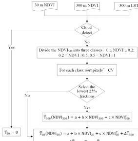
HJ-1B satellite images can provide vegetation and thermal information at spatial resolutions of 30 and 300 m, respec-tively. The 300 m resolution thermal data cannot sufficiently distinguish the surface temperatures of small targets within pixels. However, this issue can be addressed by tempera-ture sharpening based on the functional relationship between NDVI and LST. A flowchart of temperature sharpening is shown in Fig. 1, and LST at the NDVI pixel resolution can be derived based on the following steps (Kustas et al., 2003): 1. The NDVI30is aggregated to 300 m NDVI (NDVI300). Then, the NDVI300 is divided into three classes (0≤NDVI300<0.2, 0.2≤NDVI300<0.5, and 0.5≤ NDVI300).
2. A subset of pixels is selected from the scene where the NDVI is as homogeneous as possible at a pixel resolu-tion of 300 m based on the coefficient of variaresolu-tion (CV). The CVs are calculated using the original 30 m NDVI data (NDVI30) as follows:
CV= SD
mean, (1)
where SD and mean are the standard deviation and the average values of 10×10 pixels of NDVI30, respec-tively. The CVs are sorted from smallest to largest. Lower CVs correspond to more homogeneous land sur-face values, and a threshold should be determined to guarantee that a sufficient number of pixels is avail-able for least squares fitting between NDVI300andT300. Therefore, the fractions of 25 % of the lowest CVs are selected from each class.
3. A least squares expression is established between NDVI300andT300using the selected pixels.
ˆ
T300(NDVI300)=a+b×NDVI300+c×NDVI2300 (2) 4. For each 30 m pixel within a 300 m pixel,Tˆ30 can be
calculated according to Eq. (2) as follows:
ˆ
T30(NDVI30)=a+b×NDVI30+c×NDVI230+1Tˆ300, (3) where1Tˆ300=T300− ˆT300is the deviation between the regressed temperature and the temperature that was ob-served by the satellite at 300 m.
2.2 Area-weighting method based on landscape information
Coarse pixels are inhomogeneous because various types of land use may be included. Using a dominant type to represent such a large landscape is irrational. The spatial resolution of LST is significantly increased by temperature sharpening in Sect. 2.1. Consequently, all inputs of ET algorithms can be obtained at high spatial resolutions. Then, inhomogeneity is-sues can be greatly diminished by dividing the landscape into finer pixels.
Combined with a high-resolution classification map, subpixel-scale parameters can be used in the ET algorithm, which is more rational than using a dominant class type be-cause different landscapes may require different ET algo-rithms. The surface energy fluxes can be averaged linearly due to the conservation of energy (Kustas et al., 2003), and a simple average that calculates the arithmetic mean over sub-pixels is the best choice for flux upscaling (Ershadi et al., 2013). Thus, the aggregated flux at a low resolutionF (x,y)
is the arithmetic mean of all then×nsubpixel fluxes that constitute the contributing fluxF (xi,yj)at coordinate(xi,
yj):
F (x, y)= 1
n×n
n
X
i=1 n
X
j=1
F xi, yj
. (4)
Figure 1.Flowchart of temperature sharpening.
1. The VNIR and TIR input data sets are geometrically corrected and registered.
2. The area ratios of different land cover types within each pixel of a low-spatial-resolution classification image are counted.
3. According to the fine-classification data, different pa-rameterization schemes can be used in the ET algorithm to calculate the subpixel flux, such as the net radia-tion (Rn), soil heat flux (G), and sensible heat flux (H). 4. To calculate the regional flux, the flux of the large pixel is calculated by the area-weighting method as follows:
F =
n
X
i=1
wi·Fi, (5)
wherewi is the fractional area contributing fluxFi of class typeiandF is the aggregated flux at the coarse resolution. The LE is computed as a residual of the sur-face energy balance in the TSFA (see Sect. 2.3) process, in which a high-spatial-resolution image is used to re-duce the number of mixed pixels.
2.3 Pixel ET algorithm
The surface energy balance describes the energy between the land surface and atmosphere. The energy budget is com-monly expressed as follows:
Rn=LE+H+G, (6)
whereRnis the net radiation, Gis the soil heat flux,H is the sensible heat flux, and LE is the latent heat flux ab-sorbed by water vapor when it evaporates from the soil sur-face and transpires from plants through stomata. The widely used one-source energy balance model considers a homo-geneous SPAC medium and ignores the inhomogeneity and structure. In this case, LE can be expressed as follows: LE=ρcp
γ ·
es−ea ra+rs
, (7)
error introduced by the uncertainty of the surface resistance, LE is computed as a residual of the surface energy balance equation.
Rnis the difference between incoming and outgoing radi-ation and is calculated as follows:
Rn=Sd(1−α)+εsLd−εsσ Trad4 , (8)
whereSdis the downward shortwave radiation,αis the sur-face broadband albedo, εs is the emissivity of the land sur-face, Ld is the downward atmospheric longwave radiation, σ=5.67×10⁻⁸W m−2K−4 is the Stefan–Boltzmann con-stant, andTradis the surface radiation temperature.
Gis commonly estimated using the empirical relationship withRn. Because the canopy exerts a significant influence on G, the fractional canopy coverage FVC is used to determine the ratio ofGtoRnas follows:
G=Rn×[0c+(1−FVC)×(0s−0c)], (9)
where0sis 0.315 for bare soil and0cis 0.05 for a full vege-tation canopy (Su, 2002).H is the transfer of turbulent heat between the surface and atmosphere, which is driven by a temperature difference and controlled by resistances that de-pend on local atmospheric conditions and land cover prop-erties (Kalma et al., 2008). According to gradient diffusion theory, the equation forHis as follows:
H=ρcp
Taero−Ta ra
, (10)
whereρ is the density of the air;cpis the specific heat of the air at a constant pressure;Taero is the aerodynamic sur-face temperature obtained by extrapolating the logarithmic air temperature profile to the roughness length for heat trans-port;Tais the air temperature at a reference height; andrais the aerodynamic resistance, which influences the heat trans-fer between the source of the turbulent heat flux and the ref-erence height. Aerodynamic resistance was calculated based on the Monin–Obukhov similarity theory (MOST) using a stability correction function (Paulson, 1970; Ambast et al., 2002). The zero-plane displacement height,d, and roughness length,z0 m, were parameterized by the schemes proposed by Choudhury and Monteith (1988).
In this approach,H must be accurately estimated. How-ever, calculating H using Eq. (10) is difficult. Because re-mote sensing cannot obtainTaero, the value ofTaerois gen-erally replaced with the radiative surface temperature Trad, which is not always equal toTaero. The difference between these terms for homogeneous and full-coverage vegetation is approximately 1–2◦ (Choudhury et al., 1986), and it can reach 10◦ in sparsely vegetative areas (Kustas, 1990). The method that corrects for this discrepancy adds excess re-sistance rex to ra. We used the brief method proposed by Chen (1988) to calculaterex:rex=4/u∗.
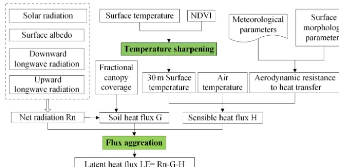
Figure 2 shows the flowchart for merging ET retrieval and temperature sharpening based on HJ-1B satellites.
The spatial-scale effect is generally revealed by a discrep-ancy between different upscaling methods. In one method, parameters are upscaled to a large scale before calculating the heat flux. In the other method, heat flux is calculated at a small scale, and the results are then upscaled. In this study, the resolution of the final output result is 300 m. To evaluate the heterogeneity-reducing effect of TSFA, two other upscal-ing methods, called IPUS and TRFA, were implemented (see Fig. 3). In the case of IPUS, the inputs of the energy balance model are first retrieved at 30 m resolution (see information of HJ-1B satellite data in Sect. 3.2.1) and then aggregated to 300 m resolution. Subsequently, these 300 m inputs are used in the one-source energy balance model to obtain the four energy balance components at 300 m resolution. In TRFA, the LST at 300 m is first resampled to 30 m using the nearest neighbor method and the 30 m resolution inputs are used for estimating ET. The outputs of the four energy-balance com-ponents of the TRFA are obtained using the area-weighting method shown in Sect. 2.2.
3 Study area and data set 3.1 Study area
Our study was conducted in the middle stream of the Heihe River basin (HRB), which is located near the city of Zhangye in the arid region of Gansu province in northwestern China (100.11–100.16◦E, 39.10–39.15◦N). The middle reach of the HRB is a typical desert–oasis agriculture ecosystem dom-inated by maize and wheat. Areas of the Gobi Desert and the alpine vegetation in the Qilian Mountains are located near the study area (see Fig. 4). The artificial oasis is highly het-erogeneous, which impacts the thermal dynamics and hy-draulic features. Consequently, the water use efficiency and ET are variable. The Heihe River basin has long served as a test bed for integrated watershed studies, as well as land surface and hydrological experiments. Comprehensive ex-periments, such as the Watershed Allied Telemetry Exper-imental Research (WATER) project (Li et al., 2009), and an international experiment – the Heihe Basin Field Exper-iment (HEIFE) as part of the World Climate Research Pro-gramme (WCRP), have been conducted in this basin. One major objective of HiWATER was to capture the strong land surface heterogeneities and associated uncertainties within a watershed (X. Li et al., 2013).
3.2 Data set
Figure 2.Flowchart of ET retrieval using the temperature-sharpening and flux aggregation method.
Figure 3.Flowchart of the three upscaling methods for retrieving evapotranspiration.
3.2.1 Remote sensing data HJ-1B satellite data
The specifications of HJ-1B are shown in Table 1. The satellite has quasi-sun-synchronous orbits at an altitude of 650 km, a swath width of 700 km and a revisit period of 4 days. Combined, the revisit period of the satellites is 48 h. Because HJ-1A/B CCDs lack an onboard calibration system, cross-calibration methods were proposed to calibrate the CCD instruments (Zhang et al., 2013; Zhong et al., 2014b). The image quality of the HJ-1A/B CCD is stable, the perfor-mances of each band are balanced (Zhang et al., 2013) and the radiometric performance of the HJ-1A/B CCD sensors is similar to the performances of the Landsat-5 TM, Observer-1 (EO-Observer-1) Advanced Land Imager, and Terra ASTER. The image quality of the HJ-1A/B CCD is very similar to the
image quality of Landsat-5 TM (Jiang et al., 2013). In ad-dition, the accuracy of the TIR band’s onboard calibration meets the land surface temperature retrieval requirements but not the sea surface temperature retrieval requirements (J. Li et al., 2011). The Center for Resources Satellite Data and Application (CRESDA) in China releases calibration co-efficients annually on its website (http://www.cresda.com). These data are freely available from the CRESDA website (http://218.247.138.121/DSSPlatform/index.html).
[image:6.612.154.441.271.466.2]Figure 4.Study area and distribution of EC towers in HiWATER-MUSOEXE.
Figure 5.Flowchart of land surface variable retrieval. The abbreviations are defined as follows: SZA: solar zenith angle; SAA: solar azimuth angle; VZA: view zenith angle; AOD: aerosol optical depth; ABT: at-nadir brightness temperature;Sd: downward shortwave radiation; USR: upward shortwave radiation; ULR: upward longwave radiation; andLd: downward longwave radiation.
Table 1.Specifications of the HJ-1B main payloads.
Sensor Band Spectral Spatial Swath Revisit range resolution width time (µm) (m) (km) (days)
CCD
1 0.43–0.52
30 4
2 0.52–0.60 360 (single) 3 0.63–0.69 700 (two) 4 0.76–0.90
IRS
5 0.75–1.10
720 4
6 1.55–1.75 150 7 3.50–3.90
8 10.5–12.5 300
The HJ-1B satellite data of the HRB were preprocessed, including geometric correction, radiometric calibration, and atmospheric correction. The following surface variables are needed in Eqs. (1) to (10): downward shortwave radiation,
downward longwave radiation, emissivity, albedo, fractional vegetation coverage (FVC), cloud mask data, meteorological data, LAI, and LST. Figure 5 illustrates a flowchart of the retrieval of these variables.
[image:7.612.49.284.521.648.2]2. The NDVI is the regression kernel of the temperature-sharpening procedure and is used to calculate the FVC. Atmospherically corrected surface reflectance values were used to calculate the NDVI as follows:
NDVI=ρnir−ρred ρnir+ρred
(11) and
FVC= NDVI−NDVIs
NDVIv+NDVIs
, (12)
where ρnir and ρred are the reflectances in the near-infrared and red band, respectively, and NDVIv and NDVIs are the fully vegetated and bare soil NDVI val-ues, respectively. As an important input for the parame-terization of surface roughness length and aerodynamic resistance, the LAI was determined using the following equation (Nilson, 1971):
P (θ )=e−G(θ )··LAI/cos(θ ) (13)
P (θ )=1−FVC, (14)
whereθis the zenith angle,P (θ )is the angular distribu-tion of the canopy gap fracdistribu-tion, G(θ )is the projection coefficient (0.5) andis the total foliage clumping in-dex, which can be obtained from the GLC global clump-ing index database accordclump-ing to the land use type (He et al., 2012).
3. Land surface emissivity (LSE) is needed to calculate the
Rn and is extremely important for retrieving LST. In this paper, LSE was calculated using the FVC as fol-lows (Valor and Caselles, 1996):
ε=εv·FVC+εg(1−FVC)+4< dε >
·FVC·(1−FVC) (15)
whereεis the LSE,< dε >is an effective value of the cavity effect of emissivity, the meandεof all vegetation species in this study is< dε >=0.015,εvandεg are the vegetation and ground emissivity, respectively. 4. Land surface temperature is a single-channel parametric
model for retrieving LST based on HJ-1B/IRS TIR data developed by H. Li et al. (2010) was employed to obtain the LST. This model was developed from a parametric model based on MODTRAN4 using NCEP atmospheric profile data.
5. Downward shortwave radiation was calculated in this study by applying the algorithm proposed by L. Li et al. (2010). MOD05, TOMS, aerosol and solar angle data were used to estimate the direct light flux and diffuse light flux using a lookup table that was generated via the 6S radiation transfer mode (Vermote et al., 2006). This method considered the influences of complex terrain, and a topographic correction was performed by using products of the ASTER digital elevation model (DEM).
6. Downward longwave radiation (Ld) was calculated by the algorithm proposed by Yu et al. (2013). The TOA brightness temperature of the HJ-1B thermal channel was used to substitute the atmospheric effective tem-perature. Effective atmospheric emissivity was param-eterized as an empirical function of the water vapor content. These values were substituted for atmospheric temperature and atmospheric emissivity to estimate the value ofLd. Because thisLdretrieval method was only valid for clear-sky conditions, cloud masking informa-tion was used to determine clear skies. When cloud con-tamination existed in the image, the brightness tempera-ture was relatively low, causing theLdto be lower than that in the cloudless images.
Ancillary data
Ancillary data were used because the bands of the satellite could not invert all of the variables needed to retrieve ET.
1. MODIS provides atmospheric water vapor data (MOD05), including a 1 km near-infrared product and a 5 km thermal-infrared product, every day. The 1 km near-infrared water vapor product was used to retrieveLdin this study.
2. For surface elevation data, we used the 30 m resolu-tion global digital elevaresolu-tion model (GDEM) based on ASTER, which covers 83◦N–83◦S, to deriveSd. 3. For atmosphere ozone data, a total ozone mapping
spectrometer (TOMS), which was carried on an Earth Probe (EP) satellite, was used to deriveSd. The TOMS-EP provided daily global atmospheric ozone data at a resolution of 1◦×1.25◦(L. Li et al., 2010).
4. For atmosphere profile data, global reanalysis data from the National Centers for Environmental Predic-tion (NCEP) were used to derive LST. These data were generated globally every 6 h (0:00, 06:00, 12:00, 18:00 UTC) for every 1◦of latitude and longitude (H. Li et al., 2010).
3.2.2 HiWATER experiment data set
The in situ HRB observation data were provided by Hi-WATER. From June to September 2012, HiWATER de-signed nested observation matrices over 30 km×30 km and 5.5 km×5.5 km within the middle stream oasis in Zhangye to focus on the heterogeneity of the scale effect in HiWATER-MUSOEXE.
Table 2.The in situ HiWATER-MUSOEXE station information.
Station Longitude Latitude Tower Altitude Land height (m) cover (m)
EC1 100.36◦E 38.89◦N 3.8 1552.75 vegetation EC2 100.35◦E 38.89◦N 3.7 1559.09 maize EC3 100.38◦E 38.89◦N 3.8 1543.05 maize EC4 100.36◦E 38.88◦N 4.2 1561.87 building EC5 100.35◦E 38.88◦N 3 1567.65 maize EC6 100.36◦E 38.87◦N 4.6 1562.97 maize EC7 100.37◦E 38.88◦N 3.8 1556.39 maize EC8 100.38◦E 38.87◦N 3.2 1550.06 maize EC9 100.39◦E 38.87◦N 3.9 1543.34 maize EC10 100.40◦E 38.88◦N 4.8 1534.73 maize EC11 100.34◦E 38.87◦N 3.5 1575.65 maize EC12 100.37◦E 38.87◦N 3.5 1559.25 maize EC13 100.38◦E 38.86◦N 5 1550.73 maize EC14 100.35◦E 38.86◦N 4.6 1570.23 maize EC15 100.37◦E 38.86◦N 4.5 1556.06 maize EC17 100.37◦E 38.85◦N 7 1559.63 orchard
GB 100.30◦E 38.91◦N 4.6 1562 uncultivated land – Gobi
SSW 100.49◦E 38.79◦N 4.6 1594 uncultivated land – desert SD 100.45◦E 38.98◦N 5.2 1460 swamp land
The station information is shown in Table 2, and the distri-bution of the stations is shown in Fig. 4. Within the artifi-cial oasis, an observation matrix composed of 17 EC tow-ers and ordinary AMSs exists where the suptow-erstation was lo-cated. The land surface was heterogeneous and dominated by maize, maize intercropped with spring wheat, vegetables, or-chards, and residential areas (X. Li et al., 2013). Because the EC16 and HHZ stations lackedRnandGobservation data, they were excluded from this study.
The ground observation data included theHand LE. Reli-able methods were used to ensure the quality of the turbulent heat flux data. Before the main campaign, an intercompar-ison of all instruments was conducted in the Gobi Desert (Xu et al., 2013). After basic processing, including spike removal and corrections for density fluctuations (WPL cor-rection), a four-step procedure was performed to control the quality of the EC data. In this procedure, data were rejected when (1) the sensor had been malfunctioning, (2) precipi-tation occurred within 1 h before or after collection, (3) the ratio of missing data was greater than 3 % in the 30 min raw record and, (4) the friction velocity was below 0.1 m s−1at night (for more details, see S. M. Liu et al., 2011; Xu et al., 2013; Liu et al., 2016). EC outputs are available every 30 min. G was measured by using three soil heat plates at a depth of 6 cm at each site, and the surface Gwas calcu-lated using the method proposed by Yang and Wang (2008) based on the soil temperature and moisture above the plates. Surface meteorological variables, such as wind speed, wind direction, relative humidity, and air pressure, were used to interpolate images using the inverse distance weighting.
Re-Table 3.The station validation results of land surface temperature.
Station R2 MBE RMSE Station R2 MBE RMSE
(K) (K) (K) (K)
EC1 0.82 0.18 1.74 EC11 0.42 1.59 2.98 EC2 0.82 0.59 1.54 EC12 0.87 0.62 1.51 EC3 0.69 0.38 1.90 EC13 0.83 0.44 1.48 EC4 0.83 −9.87 10.04 EC14 0.73 1.43 2.44 EC5 0.83 1.71 2.34 EC15 0.74 1.53 2.41 EC6 0.61 0.30 2.44 EC17 0.78 1.20 2.32
EC7 0.82 0.39 1.40 GB 0.69 0.12 2.33
EC8 0.83 0.45 1.55 SSW 0.59 1.38 3.82
EC9 0.63 2.31 3.15 SD 0.76 −3.83 4.84 EC10 0.68 1.32 2.45
searchers can obtain these data from the websites of the Cold and Arid Regions Science Data Center at Lanzhou (http://card.westgis.ac.cn/) or the Heihe Plan Data Manage-ment Center (http://www.heihedata.org/).
Energy imbalances are common in ground flux observa-tions. The conserving Bowen ratio (H/ LE) and residual clo-sure technique are often used to force the energy balance. Computing the LE as a residual variable may be a better method for energy balance closure under conditions with large LEs (small or negative Bowen ratios due to strong advection) (Kustas et al., 2012). Thus, the residual closure method was applied because the oasis effect was distinctly observed in the desert–oasis system on clear days during the summer (S. M. Liu et al., 2011).
4 Results and analysis
4.1 Evaluation of surface variables
To control model inputs and analyze error sources, the coarse-resolution land surface temperature, downward short-wave radiation, downward longshort-wave radiation, Rn, and G were evaluated using in situ data.
The ground-based land surface temperature,Ts, was cal-culated using the Stefan–Boltzmann law from the AMS mea-surements of the longwave radiation fluxes (Li et al., 2014) as follows:
Ts=
L↑−(1−ε s)·L↓ εs·σ
14
, (16)
in whichL↑andL↓are in situ surface upwelling and atmo-spheric downwelling longwave radiation, respectively, and
[image:9.612.308.545.86.212.2]Table 4.The station validation results of downward shortwave radiation.
Station R2 MBE RMSE Station R2 MBE RMSE
(W m−2) (W m−2) (W m−2) (W m−2)
EC1 0.97 25.23 27.73 EC11 0.90 30.11 33.76
EC2 0.84 28.29 33.57 EC12 0.96 24.35 26.43
EC3 0.97 17.56 19.25 EC13 0.93 12.41 17.92
EC4 0.98 6.07 9.34 EC14 0.98 32.40 33.49
EC5 0.98 10.60 12.29 EC15 0.94 26.71 29.71
EC6 0.93 27.68 30.71 EC17 0.94 −20.25 24.54
EC7 0.89 −17.69 27.59 GB 0.89 25.34 30.63
EC8 0.83 15.63 25.50 SSW 0.63 18.51 34.93
EC9 0.96 −2.27 9.96 SD 0.98 5.70 13.82
EC10 0.94 −3.50 11.97
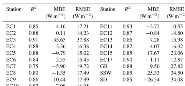
Table 5.The station validation results of downward longwave radiation.
Station R2 MBE RMSE Station R2 MBE RMSE
(W m−2) (W m−2) (W m−2) (W m−2)
EC1 0.85 4.16 17.21 EC11 0.93 −2.72 10.55
EC2 0.88 0.11 14.23 EC12 0.87 −0.84 14.80
EC3 0.91 −35.65 37.88 EC13 0.86 −7.28 15.98
EC4 0.88 3.36 16.38 EC14 0.82 4.07 16.42
EC5 0.88 −0.79 15.02 EC15 0.85 17.67 23.06
EC6 0.84 2.55 15.43 EC17 0.90 −1.11 12.87
EC7 0.75 −5.90 19.72 GB 0.88 9.50 27.82
EC8 0.80 −1.35 17.49 SSW 0.85 25.33 34.50
EC9 0.86 10.44 17.99 SD 0.85 −26.54 34.08
EC10 0.87 7.98 16.05
(2) the EC4 foundation is non-uniform and is not suitable for validation. After removing the EC4 data, theR2, MBE, and RMSE values of the LSTs were 0.83, 0.69 K, and 2.51 K, re-spectively. The LST errors of SSW and SD were large due to large errors on particular days. For example, although it was briefly cloudy above station SSW on 27 July, this area was not identified as cloudy in the cloud detection process.
The R2, MBE, and RMSE values of Sd were 0.81, 13.80 W m−2, and 25.35 W m−2, respectively. The station validation results are shown in Table 4. The accuracy of SSW is low. Because cloudy conditions occurred briefly on 27 July, few ground observations were obtained, andSd was significantly overestimated. After removing these data, the R2, MBE, and RMSE values ofSd at SSW were 0.87, 10.90 W m−2, and 21.13 W m−2, respectively.
The R2, MBE, and RMSE values of the HRB Ld were 0.73, 0.28 W m−2, and 21.24 W m−2, respectively. As seen in Table 5, the accuracies at EC3, SD, and SSW were low. The low accuracies at EC3 and SD potentially resulted from (1) high humidity, which resulted in low at-nadir bright-ness temperatures and low retrieved Ld, or (2) instrument error, which occurred because the EC3 ground observations were always greater than those of the other stations during the same period. Although SSW was located in a desert,
the ground–air temperature difference was large. TheLd re-trieval may have a large error because the models use sur-face temperature when estimatingLdto approximate or sub-stitute the near-surface temperature (Yu et al., 2013). The corrected error of ourLdretrieving algorithm resulted from the ground–air temperature difference in non-vegetated ar-eas. The inaccuracy of the SSW LST may influence theLd results.
[image:10.612.142.456.267.413.2]Table 6.The station net radiation validation results.
Station R2 MBE RMSE Station R2 MBE RMSE
(W m−2) (W m−2) (W m−2) (W m−2)
EC1 0.76 −2.55 30.61 EC11 0.86 −15.13 28.05
EC2 0.79 2.52 25.24 EC12 0.90 −8.46 19.38
EC3 0.86 −35.84 42.97 EC13 0.88 −25.73 32.34
EC4 0.84 76.64 80.25 EC14 0.90 4.23 18.18
EC5 0.85 −24.41 32.34 EC15 0.84 8.33 23.01
EC6 0.82 4.35 23.44 EC17 0.89 −62.62 68.11
EC7 0.61 −58.66 67.83 GB 0.77 −10.40 38.86
EC8 0.83 −20.62 32.45 SSW 0.44 23.05 62.93
EC9 0.87 −29.60 36.27 SD 0.75 19.98 35.24
[image:11.612.141.454.264.411.2]EC10 0.83 −24.35 33.51
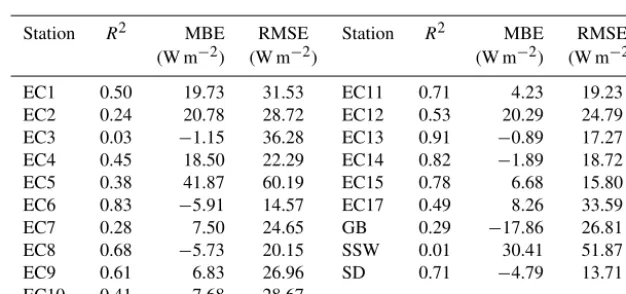
Table 7.The station validation results of the soil heat flux.
Station R2 MBE RMSE Station R2 MBE RMSE
(W m−2) (W m−2) (W m−2) (W m−2)
EC1 0.50 19.73 31.53 EC11 0.71 4.23 19.23
EC2 0.24 20.78 28.72 EC12 0.53 20.29 24.79
EC3 0.03 −1.15 36.28 EC13 0.91 −0.89 17.27
EC4 0.45 18.50 22.29 EC14 0.82 −1.89 18.72
EC5 0.38 41.87 60.19 EC15 0.78 6.68 15.80
EC6 0.83 −5.91 14.57 EC17 0.49 8.26 33.59
EC7 0.28 7.50 24.65 GB 0.29 −17.86 26.81
EC8 0.68 −5.73 20.15 SSW 0.01 30.41 51.87
EC9 0.61 6.83 26.96 SD 0.71 −4.79 13.71
EC10 0.41 7.68 28.67
by the complex vertical structure of the orchard ecosystem. The information of substrate plants may be ignored, lead-ing to albedo retrieval errors. An albedo bias of 0.03 can lead to an Rn error of approximately 20 W m−2 when the solar incoming radiation is large. As previously discussed, it was briefly cloudy on 27 July, and after removing those data, theR2, MBE, and RMSE values of theRnobtained at station SSW were 0.72, 8.20 W m−2, and 37.60 W m−2, re-spectively.
The R2, MBE, and RMSE values of theG in the HRB were 0.57, 8.51 W m−2, and 29.73 W m−2, respectively. The station-validated G results are shown in Table 7. At EC5, the soil temperature and moisture were the same at different depths after 19 July, which resulted in a surfaceGthat was equal to theGat a depth of 6 cm.Gbelow the surface was usually less than the Gat the soil surface; thus, the valida-tion results ofGat EC5 indicate thatGwas overestimated. At SSW, the brief cloudy period decreased the observed soil surface temperature, which decreased the calculated surface
G. However, the remotely sensedGdid not reflect this situ-ation. In this case, theGwas overestimated because theRn was overestimated. After removing the data on 27 July, the
R2, MBE, and RMSE values of theG at SSW were 0.17, 19.34 W m−2, and 33.30 W m−2, respectively.
4.2 Validation of heat fluxes by TSFA
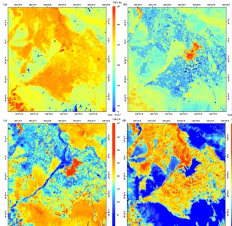
Figure 6 provides the turbulent heat flux results calculated by TSFA on 13 September 2012. The spatial distribution of the turbulent heat flux is obvious. TheH values of buildings and uncultivated land, including land patches in the Gobi re-gion, barren areas, and desert areas, were high, in addition to the LEs of water and agricultural areas in the oasis. The southern areas of the images show uncultivated barren land bordering the Qilian Mountains that resulted from snowmelt and the downward movement of water. In these areas, the groundwater levels are high and the soil moisture content is approximately 30 % based on in situ measurements at a depth of 2 cm. Therefore, the LE values of barren areas in the south are higher than the LE values of desert areas in the southeast, although both areas were classified as uncultivated land.
Figure 6.Maps of the four energy components,(a)Rn,(b)G,(c)H, and(d)LE, calculated by TSFA on 13 September 2012.
function was dispersed based on the relative weights of the pixels in which the source area was located.
The footprint validation results of the TSFA turbulent heat fluxes are shown in Fig. 7 and Table 8. TheR2, MBE, and RMSE ofH were 0.61, 0.90 W m−2, and 50.99 W m−2, re-spectively, and those of LE were 0.82,−20.54 W m−2, and 71.24 W m−2, respectively. Because LE was calculated as a residual term, it was impacted byRn, surfaceG, andH. The errors of all inputs may contribute to the LE, which compli-cates the error sources of the LE. These errors are discussed in detail in Sect. 4.3.2 and 4.4.
As shown in Fig. 7, the majority of theHvalues are small because June, July, August, and September constitute the growing season when ET greatly cools the air. The temper-ature difference between the land surface and air is small, leading to a lowH. The points with largeH values are in-fluenced by uncultivated land. In our study area, the Gobi region, barren area and desert area comprise the unculti-vated land. The points in the scatter plot with largeHvalues represent desert, where the H values reach approximately 300 W m−2. Some points in theH scatter plot are less than zero due to inversion from the oasis effect or irrigation. For example, the HiWATER soil moisture data show that
irri-gation occurred on 22 August 2012. Irriirri-gation is the main source of water within the oasis and cools the land surface to temperatures below the air temperature. In addition, irriga-tion leads to errors in LST retrieval because it increases the atmospheric water vapor content, as discussed in Sect. 4.1. The model error is further analyzed in Sect. 4.4.
Figure 7.Scatter plot of the TSFA turbulent heat flux results.
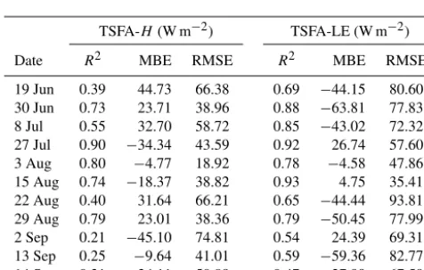
Table 8.In situ validation results of heat flux using the TSFA.
TSFA-H(W m−2) TSFA-LE (W m−2) Date R2 MBE RMSE R2 MBE RMSE 19 Jun 0.39 44.73 66.38 0.69 −44.15 80.60 30 Jun 0.73 23.71 38.96 0.88 −63.81 77.83 8 Jul 0.55 32.70 58.72 0.85 −43.02 72.32 27 Jul 0.90 −34.34 43.59 0.92 26.74 57.60 3 Aug 0.80 −4.77 18.92 0.78 −4.58 47.86 15 Aug 0.74 −18.37 38.82 0.93 4.75 35.41 22 Aug 0.40 31.64 66.21 0.65 −44.44 93.81 29 Aug 0.79 23.01 38.36 0.79 −50.45 77.99 2 Sep 0.21 −45.10 74.81 0.54 24.39 69.31 13 Sep 0.25 −9.64 41.01 0.59 −59.36 82.77 14 Sep 0.31 −34.11 50.88 0.47 27.99 67.50
4.3.1 Validation of the TRFA and IPUS heat fluxes Table 9 provides the in situ validation results of H and LE calculated using the IPUS and TRFA methods. Compared to validation results of TSFA in Table 8, the TSFA produced a better retrieval accuracy than the TRFA, and the TRFA was better than the IPUS on all days and the MBE and RMSE values of TSFA decreased and theR2of TSFA increased on most days. Table 9 shows that the improvements in accuracy between TRFA and IPUS were relatively larger than those between TSFA and TRFA. Compared to the IPUS results, the TRFA results were similar to the TSFA results because subpixel landscapes and subpixel variations of most vari-ables were considered. Thus, TRFA effectively decreased the scale error that resulted from heterogeneity because the 30 m VNIR data were fully used. However, the performance of the TRFA method is unstable. For example, on 3 and 29 August, the TRFA results were slightly worse than the IPUS results. This situation occurred because the different subpixel land-scape temperatures were considered as equal to the values estimated at the 300 m resolution. Thus, when values of LST at 300 m scale have large retrieval errors, the turbulent heat flux retrieval error may be amplified by the subpixel land-scapes.
Variations in landscape characteristics systematically trig-ger variations in surface variables. Landscape inhomogene-ity can be classified using two conditions: nonlinear vege-tation density variations between subpixels (e.g., different types of vegetation mixed with each other or with bare soil) and coarse pixels containing different landscapes (e.g., vege-tation or bare soil mixed with buildings or water). To evaluate the effects of TSFA, stations with a typical severe heteroge-neous surface at EC4, a weak heterogeheteroge-neous surface at EC11, a typical pixel (called “TP” hereafter) at the boundary of the oasis and bare soil (sample 62, line 102 in the image of study area), and a uniform surface at EC15, were selected to ana-lyze the temperature-sharpening results.
EC4 is used as an example because its land cover and sub-pixel variations of temperature were complicated. Table 10 compares the turbulent heat fluxes calculated using the IPUS, TRFA, and TSFA methods. Significant differences were ob-served between the TSFA and IPUS results and between the TRFA and IPUS results due to the heterogeneity of the sur-face. The LE calculated using the TSFA method was more consistent with in situ measurements than the LE calculated using the IPUS method because the MBE and RMSE de-creased considerably, theR2increased, and the accuracy was improved by approximately 40 W m−2. However, the LE cal-culated by the TRFA was more accurate than the LE calcu-lated by the TSFA, as discussed below.
TheH calculated by using the TSFA method was more accurate than theHcalculated by using the TRFA and IPUS methods. The RMSE of the results from the TRFA method was relatively close to the RMSE of the results from the TSFA method because the TRFA method also considers the effects of the heterogeneity of landscapes. In addition, the
Table 9.In situ validation results of the turbulent heat fluxes of IPUS and TRFA.
IPUS-H(W m−2) IPUS-LE (W m−2) TRFA-H(W m−2) TRFA-LE (W m−2)
Date R2 MBE RMSE R2 MBE RMSE R2 MBE RMSE R2 MBE RMSE
19 Jun 0.32 48.53 71.70 0.66 −47.68 86.02 0.39 52.28 70.98 0.65 −46.71 85.93
30 Jun 0.50 41.45 67.30 0.80 −81.75 102.33 0.69 42.64 60.85 0.86 −78.50 93.98
8 Jul 0.34 44.17 77.45 0.63 −66.75 118.63 0.44 54.20 76.00 0.82 −63.82 89.11
27 Jul 0.81 −33.14 50.01 0.83 25.61 74.26 0.84 −23.53 41.76 0.86 14.82 65.21
3 Aug 0.84 −5.23 33.50 0.74 −3.98 60.49 0.80 7.76 37.51 0.76 −18.23 62.71
15 Aug 0.64 −23.28 47.89 0.85 10.32 54.98 0.70 −14.77 39.99 0.89 0.59 45.22
22 Aug 0.31 41.50 74.81 0.61 −53.60 102.12 0.40 40.63 69.94 0.65 −54.17 98.97
29 Aug 0.72 27.15 44.16 0.76 −54.76 83.20 0.75 30.79 44.97 0.77 −59.43 86.22
2 Sep 0.28 −52.44 83.25 0.51 32.89 76.48 0.21 −45.77 75.84 0.52 24.37 71.69
13 Sep 0.08 −11.45 57.50 0.61 −57.38 81.83 0.06 −11.89 49.63 0.54 −57.78 84.58
14 Sep 0.12 −36.52 67.38 0.28 19.46 89.30 0.03 −34.34 64.85 0.38 25.41 75.96
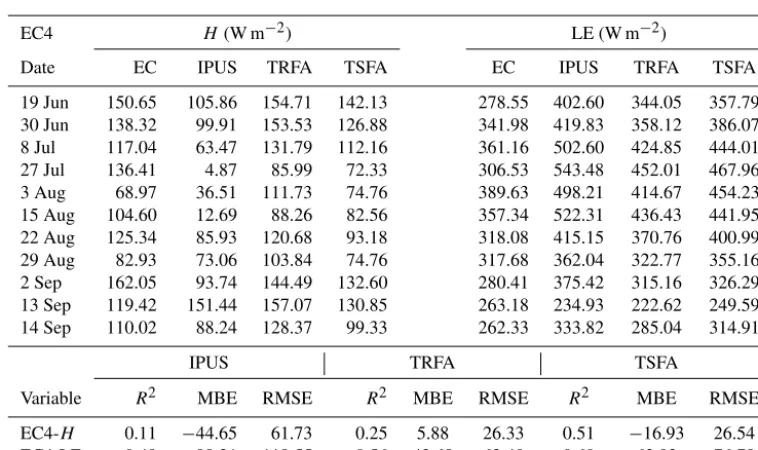
Table 10.Comparison of the turbulent heat flux results at EC4.
EC4 H(W m−2) LE (W m−2)
Date EC IPUS TRFA TSFA EC IPUS TRFA TSFA
19 Jun 150.65 105.86 154.71 142.13 278.55 402.60 344.05 357.79 30 Jun 138.32 99.91 153.53 126.88 341.98 419.83 358.12 386.07
8 Jul 117.04 63.47 131.79 112.16 361.16 502.60 424.85 444.01
27 Jul 136.41 4.87 85.99 72.33 306.53 543.48 452.01 467.96
3 Aug 68.97 36.51 111.73 74.76 389.63 498.21 414.67 454.23
15 Aug 104.60 12.69 88.26 82.56 357.34 522.31 436.43 441.95
22 Aug 125.34 85.93 120.68 93.18 318.08 415.15 370.76 400.99
29 Aug 82.93 73.06 103.84 74.76 317.68 362.04 322.77 355.16
2 Sep 162.05 93.74 144.49 132.60 280.41 375.42 315.16 326.29
13 Sep 119.42 151.44 157.07 130.85 263.18 234.93 222.62 249.59
14 Sep 110.02 88.24 128.37 99.33 262.33 333.82 285.04 314.91
IPUS TRFA TSFA
Variable R2 MBE RMSE R2 MBE RMSE R2 MBE RMSE
EC4-H 0.11 −44.65 61.73 0.25 5.88 26.33 0.51 −16.93 26.54
EC4-LE 0.49 99.21 119.55 0.56 42.69 62.40 0.60 63.92 76.78
pixels contain buildings and result in a larger 300 m reso-lution LST, and (2) the LSTs were underestimated at EC4 (as shown in Table 3), which would underestimate the value of 1Tˆ300in Eq. (3) and, consequently, the sharpening tem-perature at 30 m andH. Because the LE was calculated as a residual item in the energy balance equation, the errors of the other three energy balance components accumulate in the LE term. At EC4, the Rnwas overestimated by approximately 80 W m−2, as discussed in Sect. 4.1, but the scale effect of
Rnwas not obvious (see Sect. 4.3.2), and theGwas overesti-mated by approximately 20 W m−2. These results decreased the accuracy of the available energy and overestimated the error by 60 W m−2. Because the TRFA overestimatesH, the underestimation of H in the TSFA would result in larger overestimation of LE than that estimated by the TRFA.
Con-sequently, the LE calculated by using the TSFA method is less accurate than the LE calculated by the TRFA method.
Figure 8 shows that the classes and temperatures of 10×10 subpixels at 30 m correspond to the pixels with a resolution of 300 m at the EC tower. In the IPUS upscal-ing scheme, the 300 m pixels included buildupscal-ings, maize, and vegetable crops at the 30 m resolution and were identified as maize. The canopy height gap between maize and vegetables was large during our study period, resulting in the overesti-mation of the canopy height. For additional details, see the error analysis in Sect. 4.4. However, because buildings cor-responded with H=0.6Rn in this study, ignoring the con-tributions of buildings would result in the underestimation of
[image:14.612.111.490.283.508.2]Figure 8.Distribution of classes and temperatures over(a)EC4,(b)EC15,(c)EC11, and(d)TP on 29 August 2012.
of 313.24 K, the temperature was underestimated at a resolu-tion of 300 m. Even when substituting the in situ temperature into the ET model, the value ofHreached 399.60 W m−2and the LE became 0 W m−2. When substituting the in situ tem-perature into the TRFA method, H was 396.49 W m−2and LE was 18.7 W m−2, indicating that the LE was
based on the classification map and high-resolution inputs and correspond to more accurate sensible heat flux estimates. The land surface of EC15 was uniform and consisted of pure pixels covering maize fields. Consequently, the tem-perature distribution at 30 m resolution was very homoge-neous, and the surface temperature variations were com-prised within a range of 1.6 K. Table 11 shows the in situ validation results at EC15, for which the overall accuracy is not high due to the low LST retrieval accuracy on 8 July, which is discussed in Sect. 4.4.1. For homogeneous surfaces, the gaps between IPUS, TRFA, and TSFA were not large (within 10 W m−2), and the accuracy did not improve (MBE and RMSE did not exhibit obvious variations). Statistically sharpening the temperature may increase the uncertainty of the model results for homogeneous surfaces; however, this influence could be omitted.
The weak heterogeneous land surface at EC11 contained barley, maize, and vegetables in a 300 m pixel resolution with a fractional area of 58 : 41 : 1 and was classified as barley at the 300 m resolution. The distributions of the classes and temperatures are shown in Fig. 8c. The pixel belongs to the first conditions of heterogeneity (nonlinear vegetation den-sity variation between subpixels). Table 12 shows the in situ validation results of EC11. The improvements in the accura-cies ofH and LE by temperature resampling or sharpening were not as obvious as the improvements at EC4, which con-tained totally different landscapes (the other inhomogeneous condition).
Theoretically, the LE from the TSFA and TRFA at EC11 should be smaller than the IPUS LE values in the energy bal-ance system. The height of maize (ranges from 0.3 to 2 m) was generally higher than the height of barley (ranges from 0.9 to 1.1 m) in the study area from June to August. Taller vegetation resulted in larger surface roughness and smaller aerodynamic resistance, which led to larger H values and smaller LE values, and vice versa (e.g., vegetables with a canopy height of 0.2 m). When using the TSFA and TRFA methods, patch landscapes consisting of different crops, such as maize and vegetables, were considered. Thus, the LE was smaller than the IPUS LE. On 19 June, the canopy height of maize was 0.74 m, which was lower than the canopy height of barley (1 m) and indicated that theH values that resulted from the TRFA and TSFA methods were less thanHthat re-sulted from the IPUS method. Because our validation method considered the influence of source area, the in situ turbulent heat flux validation results included the effects of neighbor-ing pixels (i.e., on 3 August, the turbulent heat flux values of the pixel corresponding to the location of EC11 was only assigned a weight of 37 % in the source area).
The differences between the TSFA and TRFA methods were small and resulted from the LST differences between the 30 m resolution temperature-sharpening results and the LST retrieved at the 300 m resolution, but these differences were not evident at EC11. For example, on 29 August, the temperature range was 1.4 K, as shown in Fig. 8c. This
tem-perature was even less than the temtem-perature range at EC15 because the observation system at EC15 was a superstation with a 40 m tall tower that may cause large shadow effects and result in a relatively large temperature range. Hence, the temperature-sharpening effect is not obvious after aggre-gating the flux at the 300 m resolution under dense vegeta-tion canopies. However, temperature sharpening can still de-crease the heterogeneity that resulted from thermal dynam-ics.
The excess errors at EC11 was caused by the relatively low LST accuracy, withR2, MBE, and RMSE values of 0.42, 1.59 K, and 2.98 K, respectively. On August 29, the temper-ature retrieved at 300 m scale was 301.6 K, and the observed ground temperature was 300.20 K. The LST at the 300 m res-olution was slightly overestimated. When the in situ tempera-ture was substituted into the IPUS algorithm, the value ofH
decreased to 16.06 W m−2 and LE became 467.43 W m−2. When the in situ temperature was substituted into the TRFA scheme, the value ofH was 22.43 W m−2 and the LE was 461.58 W m−2, which were similar to the ground observa-tions.
Another typical pixel located at the boundary of the bare soil and the oasis with no flux measurements was used to evaluate the correction effects of landscapes and temperature sharpening. The land surface of the TP contained maize, veg-etables, and bare soil at a fraction of 35 : 31 : 34. Table 13 shows that when neither the heterogeneity of the landscape nor the LST are considered, the relative error of LE reached 180 W m−2. In addition, if only the LST heterogeneity is not considered, the LE relative error reached 48 W m−2. This result also reveals that the influences of landscape inhomo-geneity are greater than the influences of inhomoinhomo-geneity on the LST in mixed pixels.
4.3.2 Comparison of the TRFA and IPUS methods Using data of 13 September as an example, the spatial distri-butions of the four components of the energy balance calcu-lated by the IPUS and TRFA methods are shown in Figs. 9 and 10, respectively. TSFA minus IPUS and TSFA minus TRFA, which display the spatial distributions of the scale ef-fect, are shown in Fig. 11. Scatterplots of TSFA vs. IPUS and TRFA are shown in Fig. 12.
Table 11.Comparison of the turbulent heat fluxes results at EC15.
EC15 H(W m−2) LE (W m−2)
Date EC IPUS TRFA TSFA EC IPUS TRFA TSFA
19 Jun 92.55 106.60 109.25 99.81 419.47 427.19 419.99 429.98
30 Jun 42.37 43.99 45.51 44.67 551.73 527.12 525.17 526.09
8 Jul 18.34 217.53 235.48 209.90 620.95 425.71 397.49 424.86
27 Jul 27.68 21.22 31.11 24.30 597.76 589.58 579.43 586.47
3 Aug 2.33 33.32 −0.07 0.01 592.37 565.20 601.33 601.33
15 Aug 48.81 32.31 46.28 44.62 553.74 561.92 547.48 549.11
22 Aug 54.59 154.34 151.77 158.60 473.68 408.37 410.80 405.07
29 Aug 9.80 94.97 95.01 90.91 473.54 399.25 398.52 402.93
13 Sep 176.96 265.62 209.65 257.81 307.72 165.40 221.68 173.58
14 Sep 188.34 198.15 197.04 196.60 274.98 275.07 276.05 276.56
IPUS TRFA TSFA
Variable R2 MBE RMSE R2 MBE RMSE R2 MBE RMSE
EC15-H 0.40 40.64 74.64 0.33 45.93 80.81 0.40 40.36 72.88
EC15-LE 0.74 −52.11 83.48 0.71 −48.80 82.51 0.74 −49.00 81.94
Table 12.Comparison of the turbulent heat flux results at EC11.
EC11 H(W m−2) LE (W m−2)
Date EC IPUS TRFA TSFA EC IPUS TRFA TSFA
19 Jun 33.94 173.69 158.12 158.18 531.46 391.60 407.42 407.40
30 Jun 25.03 3.29 23.12 21.37 635.22 586.37 566.48 568.28
8 Jul 32.29 68.17 97.16 96.13 601.98 567.73 538.77 539.81
27 Jul 21.42 −1.17 −1.58 −3.77 587.70 618.80 619.19 621.46
3 Aug 7.01 24.85 20.34 19.52 614.28 575.03 585.29 586.16
15 Aug 38.94 12.51 15.52 16.02 567.07 584.31 581.31 580.82
22 Aug 69.25 73.45 83.11 84.38 516.07 483.23 473.60 472.40
29 Aug 29.77 48.21 60.9 60.81 473.22 427.92 415.32 415.45
2 Sep 193.97 154.58 197.01 197.49 306.62 361.96 319.54 319.03
13 Sep 288.37 168.42 176.4 177.71 160.29 216.53 208.49 207.19
14 Sep 240.33 268.91 256.29 256.40 199.52 156.00 168.63 168.55
IPUS TRFA TSFA
Variable R2 MBE RMSE R2 MBE RMSE R2 MBE RMSE
EC11-H 0.61 −1.07 61.31 0.57 −0.36 63.24 0.67 −0.21 55.50
EC11-LE 0.88 −19.83 63.16 0.89 −18.12 60.02 0.90 −21.29 58.11
heat flux by approximately 50 W m−2. Since the TSFA can integrate the effects of these land areas and reveals the rela-tive actual surface conditions, the heat flux results of TSFA vary less dramatically than those of IPUS, as shown in the figures. The results are similar in the oasis area.
Based on Figs. 6 and 10, the TRFA and TSFA methods are similar. Because the TRFA method considers the sub-pixel landscapes that could be a significant source of error in the ET models, the difference between the TSFA and TRFA methods mainly resulted from the differences between the sharpened LST and retrieved, resampled LST of subpixels at
the 30 m resolution. In addition, the bias between the TSFA and TRFA is not as obvious as the bias between the TSFA and IPUS methods, as shown in Fig. 11c–f. Furthermore, Fig. 11f shows that the LEs calculated by using the TSFA method in most oasis areas were slightly greater than the LEs calculated by using the TRFA method, which yielded values of approx-imately 20 W m−2.
[image:17.612.104.491.334.560.2]mal-Table 13.Comparison of the turbulent heat flux results at TP.
H (W m−2) LE (W m−2)
Date IPUS TRFA TSFA IPUS TRFA TSFA
19 Jun 186.31 149.73 143.98 321.04 358.22 364.79 30 Jun 383.65 191.59 158.79 67.03 259.36 292.89
8 Jul 498.36 240.20 204.18 0.29 259.25 293.41
27 Jul 276.79 136.06 84.01 206.52 347.64 402.23
3 Aug 214.14 75.45 53.72 252.37 392.08 416.41
15 Aug 214.14 98.24 72.05 252.37 368.64 393.68
22 Aug 436.48 369.28 276.70 0.00 67.79 162.80
29 Aug 235.29 117.16 67.21 183.62 302.41 356.75
2 Sep 423.61 212.15 180.92 0.00 211.77 241.36
13 Sep 338.00 285.04 216.26 0.00 53.62 122.58
14 Sep 270.44 148.20 100.19 115.19 238.43 286.51
IPUS TRFA
Variable R2 MBE RMSE R2 MBE RMSE
TP-H 0.62 174.47 185.49 0.95 42.28 48.01
TP-LE 0.71 −175.91 186.63 0.97 −43.11 49.04
[image:18.612.130.466.93.665.2]Figure 10.Maps of the four energy components,(a)Rn,(b)G,(c)Hand(d)LE, calculated using the TRFA method on 13 September 2012.
function gap. In Fig. 11, the differences of the four energy components of the pure pixels between these three meth-ods are within 5 W m−2, and the mixed pixels have different ranges.
Figure 12 shows the scatter plots between the results of the TSFA method and the other two methods for all four energy balance components. Figure 12a and e show that Rn does not vary much between the three methods and the scatter is centralized around the 1 : 1 line. However, regarding the spatial-scale effect, the differences in G,H, and LE calcu-lated by using the IPUS and TSFA methods are obvious. The scatter plots disperse at the mixed pixels, and the differences between the TRFA and TSFA results are relatively smaller. When using the TSFA method, the temperature-sharpening results can be divided into results that are higher and lower than the LST retrieved at 300 m. Compared to the LST re-trieved at 300 m when using the TRFA method, a higher LST is counterbalanced by a lower LST when calculatingH us-ing the TSFA. Thus, the effect of temperature heterogeneity is neutralized in this case. This observation is potentially re-sulted from the temperature-sharpening algorithms because they tend to overestimate the subpixel LST for cooler
land-scapes and underestimate the subpixel LST for warmer areas in the image (Kustas et al., 2003).
However, LE is calculated as a residual; thus, the differ-ence of LE is resulted fromGandH. When the 300 m mixed pixels contained various types of landscapes, they were cat-egorized as one type of landscape in the IPUS method and a single temperature value was used to evaluate the thermal dynamic effects when using the TRFA method. Pixels with highly differentG,H, and LE values are mainly distributed near the mixed pixels, as shown in Fig. 11. An explanation for these deviations is provided below.
The parameterization ofG andH are based on the land cover type. For example, for buildings,G=0.4Rn(Kato and Yamaguchi, 2005) (which is usually greater than theG of vegetation and bare soil deduced from Eq. 9) andH=0.6Rn, and for water,G=0.226Rnand LE=Rn−G. From the land cover map shown in Fig. 4, four major classes exist in the study area: buildings with a highH, uncultivated land with a relatively highH, cropland with a relatively lowH, and water withH=0.
Figure 11.Maps of the bias of the energy balance components calculated using the TSFA method minus the IPUS method:(a)Rn,(b)G, (c)H,(d)LE; and TSFA minus TRFA:(e)H and(f)LE.
are underestimated and LE is overestimated. In addi-tion, after considering the landscapes using the TRFA method, the LE is underestimated and H is overesti-mated because the pixels contain buildings that are still reflected indistinctly by LST at 300 m as the detailed temperature heterogeneity cannot be represented by the TRFA method. These points are shown in green in Fig. 12. However, if the pixel is categorized as buildup,
the building area within a pixel is exaggerated, which causesGandH to be overestimated and LE to be un-derestimated when using the IPUS method. This situa-tion is similar to that illustrated by the green points as-sociated with the TRFA results and is shown by the red points in Fig. 12.
over-Figure 12.Scatter plots between the TSFA and IPUS results:(a)Rn,(b)G,(c)H, and(d)LE; and TSFA and TRFA results:(e)Rn,(f)G, (g)H, and(h) LE. MBD and RMSD are the mean bias deviation and root mean square deviation between the TSFA and IPUS results, respectively.
estimated, G and H are underestimated in the IPUS method, and vice versa. LE is also overestimated in the pixels containing water and other types of land cover (generally bare soil in our study area). These pixels are categorized as water and are shown as blue points in Fig. 12. Some of the blue LE points calculated by using the TSFA method are slightly smaller than those calcu-lated using the TRFA method for pixels containing veg-etation. At noon, the temperature of vegetation in those pixels is lower than that of water bodies.
3. In mixed pixels that contain various crops, such as maize and vegetables, LE is underestimated if the area of maize within the pixel is overestimated because the
canopy height of the maize is taller than that of vegeta-bles. This relationship results in the overestimation of
[image:21.612.157.439.65.490.2]65.66 W m−2, and the bias between the TSFA and TRFA methods varied from 4.41 to 22.53 W m−2. More class types in mixed pixels correspond to larger biases. Table 15 shows the bias of the mixed pixels that contain buildings and bare soil between the three methods. In mixed pixels with build-ings, the IPUS and TRFA methods generally underestimated LE and had large bias values compared to those of the TSFA method. In mixed pixels without buildings and bare soil, the bias between TRFA (or IPUS) and TSFA was relatively small, which indicates that the landscape and temperature in-homogeneity were accounted for by the TSFA method. The aforementioned analyses demonstrate that the TSFA method can consider the heterogeneous effects of mixed pixels.
Considering the landscapes and inhomogeneous distribu-tion of LST, the TSFA method ensures that none of the end members (30 m pixels) are ignored or exaggerated. Thus, the distribution of LE calculated using the TSFA method is smoother and more rational than the distributions of LE cal-culated using the other methods. At the regional scale, the TSFA method describes the heterogeneity of the land surface more precisely. The degree of achievable estimation accuracy is discussed hereafter.
4.4 Error analysis
Since LE is calculated as a residual term in the energy bal-ance equations, the sensitivity ofH was analyzed first. Land surface variables (including LST, LAI, canopy height, and FVC) and meteorological variables including wind speed, air temperature, air pressure, and relative humidity are the major factors forH sensitive analysis. Figure 13 presents a case of sensitivity analysis results forH. In this case, LST is 303.9 K, and it ranges from 298.4–309.4 K with a step size of 0.5 K, LAI is set to 1.4 and it ranges from 0.14–2.66 with a step size of 0.14. Canopy height is 1 m and it ranges from 0.1–1.9 m with a step size of 0.1 m. Additionally, FVC=0.5, wind speedu=2.48 m s−1, air temperatureTa=297.9 K, air pressure=97.2 kPa, and RH=40.29 %. In addition, the land cover is maize, and the referenceH is 230.2 W m−2.
The air pressure is stable over a short period and has lit-tle effect on the ET results. Although excess resistance was calculated from the friction velocity, the meteorological data were provided by ground observations; thus, the meteorolog-ical data are relatively accurate. As shown in Fig. 13, LAI, canopy height, and LST are sensitive variables.
The parameterization of the momentum roughness length indicates that H is sensitive to LAI, with decreasing sen-sitivity when the LAI is greater than 1. When the LAI is less than 1, the momentum roughness length increases as the LAI increases, and turbulent exchange is enhanced. How-ever, when the LAI is greater than 1, the plant canopy is re-garded as a continuum that is not a sensitive variable. Be-cause our study area is dominated by agriculture and the study period extended from July to September, the crops in the HRB middle stream grew quickly, thus, the LAI was
usu-ally greater than 1. Thus, LST and canopy height are the main sources of error.
4.4.1 Errors in LST
As shown in Fig. 13, 1 K LST bias would result in 21 % error ofH whileH is 230.2 W m−2. However, the sensitivity of the LST is unstable and depends on the strength of the turbu-lence. The strength of the turbulence determines the mass and energy transport and the resistance of heat transfer, which in-fluences the sensitivity to the LST. A weaker turbulence cor-responds to a weaker LST sensitivity, and vice versa.
A sensitivity analysis of LE induced by LST was also per-formed. In order to exclude the influence of other factors, stations were chosen with homogeneous landscapes within coarse pixels. These results are shown in Table 16. The LE results obtained from the observed LST are consistent with the in situ observations and have less bias. LE was overes-timated when the LST was underesoveres-timated, and vice versa. Because the magnitude of LE was greater than that of H, the relative error of LE was less than the relative error ofH. However, 1 K of LST bias resulted in an average LE error of 30 W m−2, which is consistent with the sensitivity anal-ysis of H shown in Fig. 13. Specifically, 1 K of LST bias would result in an LE biases of 8.7 W m−2(in desert, SSW) to 84.4 W m−2(in oasis, EC8), which indicates that the sen-sitivity of LST is unstable.
4.4.2 Errors in canopy height
In this paper, canopy height was obtained from a phenophase and classification map. Thus, the accuracy of the canopy height was mainly dependent on the classification accuracy and plant growth state. Even within the same region, the canopy height of a crop can differ due to differences in seed-ing times and soil attributes, such as soil moisture and fertil-ization.
The land use type was orchard at EC17. However, in our land classification map, the land use at EC17 was other crops, which includes vegetables and orchards. Thus, it was diffi-cult to set the canopy height. In our study area, most of the other crops were vegetables (canopy height of 0.2 m), and the height of the orchard was approximately 4 m; thus, a value of 0.2 m would overestimate the LE. The LE estimations with incorrect canopy heights and correct orchard canopy height at EC17 are shown in Table 17. The days of large LST bias were removed, and the bias between the model and ground observations decreased. The excess errors were caused by er-rors in the LST and land use, such as buildings and maize in the mixed pixels.
Except for the error source discussed previously, the fol-lowing sources of error were unavoidable:
Table 14.Comparison of the latent heat flux in pixels containing different numbers of class types.
Number IPUS (W m−2) TRFA (W m−2) Pixel
of class R2 MBD RMSD R2 MBD RMSD number
types in pixels
1 1.00 0.21 0.21 1.00 0.05 0.61 11 398
2 0.85 −7.18 35.36 1.00 −0.35 4.41 8212
3 0.66 −2.32 52.55 0.98 −7.33 12.56 4762
4 0.49 1.88 65.66 0.96 −11.56 16.55 2824
5 0.98 −30.92 62.69 0.96 −16.90 22.53 4
[image:23.612.103.497.272.491.2]Notes: the number of class types in mixed pixels represents the number of classification types that were contained in the pixels. For example, 1 represents the pure pixels and 2 represents mixed pixels containing two land use types. MBD and RMSD are the mean bias deviation and root mean square deviation, respectively, between the TSFA results and the TRFA and IPUS results.
Table 15.Comparison of the latent heat fluxes of typical mixed pixels.
Types of mixed pixels IPUS (W m−2) TRFA (W m−2) Pixel
R2 MBD RMSD R2 MBD RMSD number
Mixed pixels containing buildings 0.58 −1.02 61.94 0.97 −9.64 14.66 4918 Mixed pixels not containing buildings 0.81 −5.49 39.21 0.99 −2.12 7.60 10 884 Mixed pixels containing bare soil 0.73 −1.52 49.04 0.98 −5.96 11.86 9049 Mixed pixels not containing bare soil 0.65 −7.55 45.28 0.98 −2.46 7.83 6753
Figure 13.Sensitivity analysis of the surface variables for sensible heat flux.
2. The calibration coefficients of the HJ-1B satellite’s CCD and IRS drifts because of instruments aging. 3. Geometric correction causes half-pixel bias equal to or
less than the deviation of the artificially subjective inter-pretation.
A one-source model and simplified parameterization schemes were used in this paper to determine surface rough-ness lengths and heat transfer coefficients. The one-source model combines soil evaporation and plant transpiration and assumes that SPAC is a one-source continuum. This assump-tion is reasonable when the surface is densely covered by vegetation but relies on the accuracy of the difference be-tween the LST and air temperature, as previously mentioned. When a one-source model is applied to an area covered by
sparse vegetation, such as semiarid or arid areas, this assump-tion is irraassump-tional.
5 Discussions