Positive Impact Program Evaluation

ScholarWorks @ Georgia State University

ScholarWorks @ Georgia State University

Geosciences Theses Department of Geosciences

Fall 12-20-2012

Urban Stream Channel Geomorphology: Investigating the

Urban Stream Channel Geomorphology: Investigating the

Short-Term Channel Stability and Bed-Material Transportation within a

Term Channel Stability and Bed-Material Transportation within a

Rehabilitated Urban Stream Reach in DeKalb County, Georgia

Rehabilitated Urban Stream Reach in DeKalb County, Georgia

Andreas Shoredits Georgia State University

Follow this and additional works at: https://scholarworks.gsu.edu/geosciences_theses

Recommended Citation Recommended Citation

Shoredits, Andreas, "Urban Stream Channel Geomorphology: Investigating the Short-Term Channel Stability and Bed-Material Transportation within a Rehabilitated Urban Stream Reach in DeKalb County, Georgia." Thesis, Georgia State University, 2012.

https://scholarworks.gsu.edu/geosciences_theses/55

AND BED-MATERIAL TRANSPORTATION WITHIN A REHABILITATED URBAN STREAM REACH IN DEKALB

COUNTY, GEORGIA

by

ANDREAS S. SHOREDITS

Under the Direction of Jordan A. Clayton

ABSTRACT

Rivers and streams are sensitive to alterations in their watersheds and one of the greatest

disturbances is from urban development. An urban stream channel in the Atlanta metropolitan area in

the Georgia Piedmont was studied to establish the nature of adjustment the channel form was

experiencing. This study compared a degraded channel with a channel influenced by stabilization efforts

in the same stream reach, in order to investigate the behavior of channel adjustments towards a greater

stability. Measurements of the short-term changes in channel cross-sectional area and bed-material

volume, following a series of threshold flow events, were taken in the reach and the variation in bed

sediment texture was also investigated. Results showed that channel banks were stable compared to

more mobile beds and that urban effects continued to dictate sedimentation. Rehabilitation measures

were aggrading channels in their reaches and were likely perpetuating the instability of upstream

channels.

AND BED-MATERIAL TRANSPORTATION WITHIN A REHABILITATED URBAN STREAM REACH IN DEKALB

COUNTY, GEORGIA

by

ANDREAS S. SHOREDITS

A Thesis Submitted in Partial Fulfillment of the Requirements for the Degree of

Master of Science

in the College of Arts and Sciences

Georgia State University

Copyright by Andreas Stefan Shoredits

AND BED-MATERIAL TRANSPORTATION WITHIN A REHABILITATED URBAN STREAM REACH IN DEKALB

COUNTY, GEORGIA

by

ANDREAS S. SHOREDITS

Committee Chair: Seth E. Rose

Committee: Jordan A. Clayton

Daniel M. Deocampo

Leslie A. Edwards

Electronic Version Approved:

Office of Graduate Studies

College of Arts and Sciences

Georgia State University

ACKNOWLEDGEMENTS

I must extend a great thank you to my advisor, Dr. Jordan Clayton, for his valued support during

my study, his guidance in the field, and especially his continued communication with me over the past

year from Salt Lake City, UT. Without the help of Barrett Fisher my field data collection would have been

less successful and certainly less adventurous. I commend his eagerness towards the field work and his

tireless efforts out there with me. Mr. Ed Segraves has contributed to the success of this study by

making his property available to me and through his promotion of research on this mitigation banking

site. His property was made accessible to me at my convenience and I thank him for this. Dr. Seth Rose

has provided me with continued guidance throughout my graduate career including, but not limited to,

teaching advice and industry preparedness. His wise counseling has always been appreciated. My

committee has continuously provided me with valuable feedback during the progression of my thesis

work and for this they have my gratitude. A further thank you is extended to my department, the

Department of Geosciences, for providing the necessary equipment and funding for me to have

effectively conducted my field work and for who’s members helped me advance through this M.S.

program. Lastly, my brother Stefan has provided me with ongoing support and I appreciate this

TABLE OF CONTENTS

ACKNOWLEDGEMENTS ... iv

LIST OF TABLES ... vii

LIST OF FIGURES ... viii

1 INTRODUCTION ...1

1.1 Purpose of the Study and Thesis Question ...2

1.2 Background on Urban Streams and Stream Rehabilitation ...4

1.3 Site Selection and Description ...5

1.4 Literature Review ... 11

2 METHODS ... 13

2.1 Channel Cross-Section Analysis ... 13

2.2 Sediment Volume ... 16

2.3 Grain-size Distribution ... 16

2.4 Stream Stage and Water Surface Slope ... 18

2.5 Effective Stream Discharge ... 20

2.6 Rapid Geomorphic Assessment ... 21

3 RESULTS ... 23

3.1 Channel Cross-section Analysis ... 23

3.2 Sediment Volume ... 38

3.3 Grain-size Analysis ... 40

3.3.1 Bed-material Subsurface ... 40

3.4 Rapid Geomorphic Assessment ... 44

4 DISCUSSION... 47

5 CONCLUSION ... 52

REFERENCES ... 54

APPENDICES ... 58

Appendix A ... 58

Appendix B ... 60

LIST OF TABLES

Table 1 – Results from the cross-sectional resurvey analysis ... 33

Table 2 - Channel sediment volume densities ... 39

Table 3 - Rapid Geomorphic Assessment (RGA) results for the Snapfinger Creek Mitigation Bank ... 46

Table B1 – Pre-flood sample analysis ... 60

Table B2 – Post-flood sample analysis... 61

Table B3 – Pre-flood pebble count analysis ... 62

Table B4 – Post-flood pebble count analysis ... 63

Table C1 - Statistical analysis of cross-section resurvey results ... 64

LIST OF FIGURES

Figure 1.1 – Study location in the state of Georgia ...7

Figure 1.2 – Map of the study reach ...8

Figure 3.1 – Control Site cross-sectional analysis ... 26

Figure 3.2 – Control Site sketch... 26

Figure 3.3 – North Experimental Site cross-sectional analysis ... 29

Figure 3.4 – North Experimental Site sketch ... 29

Figure 3.5 – South Experimental Site cross-sectional analysis ... 32

Figure 3.6 – South Experimental Site sketch ... 32

Figure 3.7 – Plot of channel area alterations ... 34

Figure 3.8 – Plot of volumetric channel changes per cross-sectional segment ... 35

Figure 3.9 – Grain-size distribution plots ... 43

Figure 3.10 – Channel bed surface gravel analysis ... 44

1 INTRODUCTION

As rural populations dwindle at the expense of increasingly urbanizing populations it is expected

that by 2025 85% of the U.S. population will be considered urban (United Nations, 2012). Between 2000

and 2008 the southern U.S. experienced the largest regional population increase in the nation

(11.5 million) according to the 2009 U.S. census (O'Driscoll et al., 2009). Typically the urbanization of

watersheds is associated with a multitude of alterations in the hydraulic regime of stream channels and

associated channel instabilities which will affect the maintenance of aquatic habitats (Wolman, 1967;

Rose and Peters, 2001; Leopold et al., 2005; Chin, 2006). The term ‘stability’, in terms of stream

channels, implies that a channel form is essentially constant or temporarily balanced under current

conditions (Henshaw and Booth, 2000; Niezgoda and Johnson, 2005). Rivers and streams that have been

modified by human intervention will undergo progressive channel modifications towards greater

stability over a much shorter time-span compared to modifications related to more natural

disturbances. This makes urban streams ideal settings for studying the balance between channel

sediments changes and channel morphology alterations as these stream channels develop into more

stable forms (Simon, 1989).

The normal adjustment of degraded urban streams are frequently cut short by additional human

intervention in the form of channel stabilization or stream restoration measures to limit property

damage, control unpredictable flows or rehabilitate lost ecological settings (Niezgoda and Johnson,

2005; Bernhardt and Palmer, 2007). Practices such as stream restoration have notoriously been linked to

a dearth of sufficient monitoring data needed to assess the degree of post-project effectiveness, and

thus restoration efforts can conceivably also contribute towards further channel degradation. A

common approach in understanding the propensity towards channel stability, particularly in urban

flow and sediment imbalances (Henshaw and Booth, 2000). Reach instability can include incision of the

channel bed, bank erosion or failure, and an increased sediment transportation competency. Many of

these cases of instability are communicated by comparisons of temporal and spatial channel

cross-sectional change and others by channel bed-material sediment investigations. Grain size changes are

important for many reasons including the inhibition of a channel equilibrium geometry, influences on

sediment transport capacity, implications for biological communities, and because changes in grain size

distributions represent a degree of freedom in channel responses to channel disturbance (Doyle and

Shields, 2000). The fundamental cause for bed material change, other than just increased high flows,

would be the sediment supply derived from watershed development contributions.

This purpose of this study was to evaluate the dominant processes taking place in a stream

channel affected by watershed urbanization, and to assess the current stability of the reach through

inspection of changes in channel areas and the movement trends of bed sediments. In addition this

research explores whether reach-scale stream restoration practices are likely having a positive or

negative feedback on an existing degraded stream system.

1.1 Purpose of the Study and Thesis Question

The current research investigates whether the short-term adjustments in stream channel

volume in conjunction with bed sediment transportation could, after a series of threshold flow events,

be utilized to assess the stability of a restored reach in an urbanizing watershed. This premise is based

on comparing a channel reach in a degraded stream, where watershed-scale anthropogenic

disturbances continue to exert their indirect control, to a channel reach in the same stream that has

been influenced by reach-scale anthropogenic stabilization efforts such as stream restoration.

Quantification of channel capacity modifications (by cross sectional comparison) and an analysis of

stabilization efforts on the stream channel or that the same channel is still largely adjusting to

watershed urbanization.

A ‘stable’ morphology would imply that the channel form no longer undergoes progressive

adjustments, such as with bed and bank erosion, and it is essentially in a state of dynamic equilibrium

(Wolman, 1967; Schumm, 1977; Henshaw and Booth, 2000; Rakovan and Renwick, 2011). Stream

channels which have, for example, historically been destabilized as a result of increased impervious

surface cover following watershed urbanization, will over a period of some years have adjusted their

channel form to a state where there is neither a propensity towards aggradation nor degradation

(Church, 2006). It may take decades for urban rivers and streams to restabilize (Ruhlman and Nutter,

1999; Chin, 2006), and unless there is sufficient prior knowledge of pre-disturbance channel conditions,

predicting required time-periods for increased stability becomes improbable. Reaches adjusting to

variable external controls will attain what is known as a quasi-equilibrium state in their channel

geometry and hydraulic processes (Knighton, 1998; Leopold et al., 2005; Annable et al., 2012). In many

cases it has been possible to frame these newly equilibrated channel hydraulic geometries and bedload

characteristics in terms of stages in a channel evolution model (CEM) for incised channels developed by

Schumm et al. (1984) and modified by Simon (1989, 1994) (Simon, 1989; Doyle and Shields, 2000;

Mukundan et al., 2011). Given enough time and space to adjust (Niezgoda and Johnson, 2005),

degraded urban channels can be analyzed based on stage classification thus permitting certain

predictions on the long-term responses associated with channel sediment and discharge dynamics.

Work by Annable et al. (2012) postulates that even with the profuse and rapid urbanization of

watersheds currently taking place, there are still too few studies that expand on our knowledge of urban

channel stability in terms of a quasi-equilibrium condition. Bledsoe and Watson (2001) admitted that

measured data of urban influences on stream channel form are lacking, which means that our

upon. The current study on a restored reach in Snapfinger Creek in DeKalb County, Georgia, aims to

identify the current state of stability at a reach-scale and to apply these findings as a prediction relating

to a larger spatial- and temporal scale for this urban stream. It should be noted that this study is not

intended as an unequivocal evaluation of the success and failures of restoration efforts at Snapfinger

Creek, but is rather a study of the nature of channel topography adjustments in a unique setting where

both urban and restoration dynamics are at play.

1.2 Background on Urban Streams and Stream Rehabilitation

Urban stream channels differ from streams flowing through less impacted landscapes because

they are affected by a unique set of watershed impacts and both physical and cultural constraints.

Stream channels found in cities drain low-permeability watersheds that in turn produce flashy

hydrographs and reduced baseflow conditions (Rose and Peters, 2001; O’Driscoll et al., 2010).

Impervious surface coverage regularly accompanies watershed development and transmits the larger

volumes of runoff even during ordinary precipitation events. The receiving stream channels become

greatly enlarged as their ecosystems become increasingly degraded by diminished water quality

conditions and the removal of riparian vegetation (Wolman, 1967; Leopold et al., 2005; Violin et al.,

2011).

The impacts of urbanization on streams typically follow an evolution of alteration phases or

stages in characteristic channel morphologies (Simon, 1989; Doyle and Shields, 2000). Initial

construction and urban expansion produces sedimentation of drainages with large quantities of sand

and associated stream channelization. With completion of construction, sediment sources are decreased

as the amount and efficiency of runoff is increased as channel beds and banks begin to degrade as

streams become incised (Wolman, 1967). Over time the material contributed by channel enlargement

flows tend to selectively remove finer grains from a generally increasingly coarse channel bed and,

because of a reduction in stream power aided by coarse sediments, the reach approaches a

quasi-equilibrium condition as a more dynamic form of channel stability (Simon, 1989; Chin, 2006; Annable et

al., 2012). As each developing watershed is unique pertaining to the degree and rate at which urbanizing

is taking place (in addition to many other factors), urban stream channel responses will vary both

spatially and temporally in achieving a more stable form.

1.3 Site Selection and Description

Snapfinger Creek has its watershed in the headwaters of the Upper Ocmulgee river basin

located in north central Georgia (Figure 1.1). This 4th order stream (Eco-South Inc., 2007) feeds into the

Ocmulgee River basin which ultimately forms the Altamaha River towards the Atlantic coastline to the

southeast. The total watershed area covers approximately 100 km2 (U.S.EPA, 2010) and it is underlain by

Southern Piedmont-Blue Ridge province geologies of the late Proterozoic and early Paleozoic Atlanta

Group including the Clairmont, Wahoo Creek, and Clarkston Formations, together consisting largely of

gneisses, schists and amphibolites (McConnell and Abrams, 1984). The watershed drained by Snapfinger

Creek and its two main tributaries (Indian Creek and Barbashela Creek) lies entirely within DeKalb

County and comprises approximately 38% urban land use (Trawick, 2009) with largely sub-urban

residential and light industrial developments. According to the U.S. EPA 2010 watershed assessment

report for the Upper Ocmulgee, Snapfinger Creek was listed as ‘impaired’ due to high pathogen and low

stream biota counts and in 2000 it was listed as having high counts of heavy metals (U.S.EPA, 2010). The

urban nature of this stream is further demonstrated by its flashy flow response to rainfall events.

In August 2009, the Snapfinger Creek Mitigation Bank (SCMB) was completed on a reach in the

lower third of the Snapfinger Creek watershed. The roughly 62.7 hectare restoration site is located

of the metropolitan perimeter (Figure 1.2). The property is bordered to the south by the I-20 overpass at

which point the interpolated drainage area of Snapfinger Creek is 81.8 km2 (Carter et al., 1986).

Mitigation efforts sought to restore lost forested, bottomland hardwood wetlands habitats and

impacted stream functions to this former golf course (Eco-South Inc., 2007; U.S.FWS, 2012). Primary

objectives in restoring the Snapfinger Creek reach were to stabilize the largely eroding banks along the

reach by implementation of around 630 linear meters of both traditional and bio-engineering features

which included rock vanes, root-wads, geotextiles and log-revetments (Eco-South Inc., 2007). Many of

the bank-engineering functions, such as the establishment of riparian vegetation and the prevention of

excessive bank erosion, were compromised by the occurrence of a large flood event in September of

Figure 1.1 – Study location in the state of Georgia

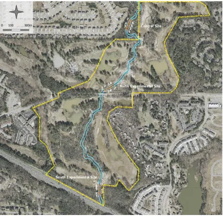
Figure 1.2 – Map of the study reach

Satellite image of the study reach and the three channel sites. The yellow boundary demarks the mitigation bank property and the numbered orange lines denote the approximate cross-section setup for each site (2010 orthoimagery courtesy of U.S. Geological Survey).

Snapfinger Creek comprises largely sandy channel material with very apparent ripple bed-forms

covering the channel bed. Sand dominated bed-material regularly becomes fully mobilized over a broad

range of flows as it moves in the form of sand sheets and suspended material. Channels characterized by

bed sediment which moves as mixed loads are known as transitional channels. An abundant supply of

sand tends promote bed instabilities by increasing bed–material mobility and the accompanied

migration of bed-forms (Church, 2002, 2006).

Three channel locations were investigated to study the sediment transportation potential in this

restored reach. The study design incorporated a comparison of restored with non-restored portions of

the same urban stream. It should be noted that the term ‘restored’, in this study, is used to refer to

reaches on which mitigation intervention has been practiced and does not indicate the absolute stability

of those sections of Snapfinger Creek. Two experimental sites known as the North Experimental Site

(NES) and the South Experimental Site (SES) would examine the channel adjustments taking place near

the middle and lower reaches in the mitigation bank respectively. Upstream of the restoration site,

reaches were unaffected by direct stabilization efforts and were therefore suited as a control for

alterations due to intervention downstream. The Control Site (CS) was located ±120 m upstream of the

property boundary where the predominant influence on channel dynamics would be from urbanization

rather than from restoration efforts (Figure 1.2).

Two criteria were used for selecting study sites and these were based on the field observations

conducted before the study commencement. The first requirement was that sites had a relatively

straight channel section in order to limit the influence of geomorphic effects which may have

complicated the interpretation of perceived stability observations (O’Driscoll et al., 2009). Any

geomorphic flow hydrology controls would also have obscured the effects of urban-induced processes

with more natural processes of channel alteration (Henshaw and Booth, 2000). The second requirement

excessive bank-protection engineering. By meeting these requirements each survey channel would likely

not conform to the conventional reach study length of 20-50 channel widths and a cross-sectional

spacing of two to five channel widths as used by other field investigators (Kondolf and Micheli, 1995).

Actual sites for this study amounted to shorter reach lengths and cross-section spacing for field

measurements (Figure 1.2).

The Control Site (CS) reach was chosen based on (i) its proximity to the mitigation site but and

(ii) that it exhibited the typical channel morphology of a degraded urban stream. This channel exhibited

deeply incised channel depths (±2.51 m), fairly narrow channel widths (±12.9 m), and significant tilted

and fallen trees. The eastern banks were well vegetated and primarily composed of sand deposits that

were likely derived from historic meander alluvium. In contrast, the western banks were taller and

composed of cohesive, red ultisols with steep bank failures. Along these banks it was common to find

severely undercut tree roots with large trees essentially suspended above the outer channel. This site

typified an urban stream channel that was not yet adjusted to frequent high flows and had experienced

significant vertical incision with bank failures. Bed sediments were mostly fine to coarse sands and silts

and characteristic features in this reach included sand/silt bed-forms which seemed to aggrade down

channel.

The North Experimental Site (NES) was situated near the midpoint of the stream mitigation

property (Figure 1.2) and it represented a reach that was directly downstream of the majority of bank

engineering practices in the reach. The channel was fairly shallow (±1.86 m) and broad (±14.9 m)

compared to the CS dimensions, and bank material consisted mainly of non-cohesive sands with well

vegetated banks. This site had some notable features which included: (i) a coir-fiber log protecting

almost the entire length of the left bank toe, (ii) that it was immediately downstream of a channel step

in the form of rock weir, (iii) an in-stream tree as a result of prior bank collapse, and (iv) two large

At approximately 85 m north of the I-20 overpass towards the southern end of the mitigation

property, the SES constituted the most downstream culmination of possible mitigation effects on

channel dimensions and bed composition. This channel reach was shallower (±1.8 m) and broader

(±16.1 m) than both upstream sites and some bank stabilization features such as log revetments,

remnant bank rip-rap and a few geotextile bank coverings were present. Relatively few flow obstacles

existed in this channel compared to the other study sites and riparian vegetation was generally well

established except for a clearing along the upper-most part of the reach. All the study sites had beds

with clearly developed ripples comprising the largely sandy bed-material surface and rip rapped portions

of the banks in all three sites were unavoidable. Bed surface compositions also maintained shifting

gravel clusters (surface material >4.0 mm) which were particularly apparent in both experimental sites.

1.4 Literature Review

Doyle and Shields (2000) produced a study to develop a modified version of the Channel

Evolution Model (CEM) based on the inclusion of qualitative predictions of bed textural changes which

incising rural channels experience as they progress through the geomorphic evolution as described by

Schumm et al. (1984) and later revised by Simon (1989, 1994). In their study three reaches in eastern

Mississippi were chosen for the sake of comparison with a study done on the same reaches a decade

before and the current study attempted to replicate these previous study procedures. It was found that

the prediction of longitudinal grain size distribution did not follow the conventional down-stream fining

trends observed by others, and the dominant factor in in the development of grain size distributions was

rather attributed to the sediment sizes, quantities, and their source locations within the watershed.

Although grain size plays a larger role than previously appreciated in the evaluation of incised channels,

Numerous contemporary papers are centered around evaluating the effectiveness of stream

rehabilitation projects, often supplementing for the general lack of existing post-project monitoring

data (Bernhardt et al., 2005). One such study by Buchanan et al. (2012) investigates a suite of

geomorphic parameters in order to identify the success of project objectives in central New York State,

two years after rehabilitation efforts. It was found that the restored reach experienced excessive overall

degradation, especially in the upper reach, and aggradation at the bottom of the reach likely resulting

from local scour higher up. Low bed and bank stability throughout the reach may have been attributed

to ‘hard’ engineering structures such as cross- and bank vanes, which promoted accelerated incision of

scour pools and inadvertently deflected high flows onto banks. The resulting short-term channel

instability did not, however, undermine the outlook for long-term success but rather emphasized the

importance of accounting for sediment transport and watershed-scale stressors.

A study by Miller and Kochel (2010) evaluates 26 stream mitigation sites in North Carolina, many

of which have suffered from large post-project adjustments in channel capacity over a timespan of one

to six years since project completion. By examining channel dimension changes through time, the

authors investigated the short-term stability and the long-term likelihood of equilibrated channel

conditions. In many of the examined reaches there was a re-organization of channel form, configuration,

and slope in the form of localized amounts of scour and fill. Changes in channel capacities were

particularly related to increases in slope, bed grain size and project age and in this study the time

required for channels to reach equilibrium exceeded the monitoring period. The recovery of highly

dynamic channels was deemed near impossible to instigate save for properly addressing three

influential parameters, namely excess shear stress (e.g. flashy urban channels and high gradient

streams), sediment supply (e.g. historic land-use changes upstream), and bank erodibility (the degree of

2 METHODS

2.1 Channel Cross-Section Analysis

Cross-sectional measurements were used to determine the changes that were occurring in

channel areas and were taken using auto-level surveys at seven transects with a spacing of 10 m

(permitting there were no major obstacles) along the length of three 60 m reaches. The transect spacing

was determined from an initial inspection of the NES reach channel width, which helped establish that

cross-sectional spacing should be at least 8 m apart which would equal approximately one-half of the

channel width. To measure each transect, a stake was set on either side of the channel which was

spanned by a surveying tape across the entire width of the channel starting from the left bank side. An

auto-level was positioned on either bank to clearly sight both stakes on opposing banks of the transect.

The entire length of the measuring tape, spanning each transect, needed to be visible without

obstruction. To maintain a consistency in measurements, each completed cross-section was calibrated

by checking the instrument’s elevation against a site benchmark location (BM). Benchmarks were

commonly chosen to be the tops of adjacent stakes or other more permanent features such as trees or

signage postings. A stadia rod was used to measure the changes in elevation across the cross-section

and elevation readings are compared to a predetermined datum (the top of the left bank stake in this

case). Two persons were responsible for conducting these measurements, with one at the surveying

station and the other walking each cross-section with the stadia rod taking depth measurements. The

person walking along the channel transect decided at what intervals and thus at what resolution

readings were taken at various locations in the channel. To ensure that transect monuments could

withstand overbank flows so that future measurements could be taken, staked locations were

reinforced with rebar rods. GPS coordinates were collected for all auto-level surveying sites so that the

Any potential changes in channel area would depend on the threshold for entrainment of bed-

and bank-material imposed by stream channel flow. Consequently, this study was constructed around a

period of flow events that were effective in moving channel sediments to a measurable degree (this is

described in greater detail below). The terminology used in the study describes ‘pre-flood’ and

‘post-flood’ measurements in association with initial channel conditions and those conditions representing a

period of effective flow events, respectively. To calculate the amount of change in cross-sectional areas

for each transect, an area calculation was performed in a spreadsheet whereby the channel depth was

set to bank scour lines representing some high flow stand in the NES channel. The use of a scour line to

represent the cross-section area was considered more representative than using a determined bankfull

flow as it is well known that bankfull stages are difficult to estimate based on specific return intervals in

urban environments (Annable et al., 2012). The flashy hydrology of urban streams makes determining a

bankfull-flow recurrence interval for these channels less reliable than for channels with less variable

flows (Shields Jr et al., 2003). The scour lines in the NES measured 1.92 m in channel depth and the

wetted channel perimeter at this stage was thought to be representative of pertinent changes in

channel form, as bank vegetation above this line appeared more established. The water surface height

at this stage was used as the datum for calculating cross-sectional area changes. As no major tributaries

entered the study reach, a continuity of steady, uniform flow through the reach was assumed with a

discharge (Q) that was relatively constant for each site. Appropriate bank heights for the remaining

reach cross-sections were estimated using the continuity equation in Equation 1, where these heights

were approximated from resulting areas (A) using the calculated velocity (v) and a uniform discharge

value (Q). The calculations utilized to establish cross-sectional areas were:

Q = vA (1)

where Q = flow discharge (m3/s), v = flow velocity (m/s), A = the channel area of the wetted perimeter

(m2), k = 1 m1/3/s (for SI), R = hydraulic radius, S = channel slope, and n = Manning’s roughness value.

Initial calculations required determining the flow velocity (v) for the NES using the Manning equation

(Equation 2) and this value was established by: (i) using the measured channel slope (S = ±0.001), (ii)

calculating the hydraulic radius (R) relating to the bank scour height where A = 26.1 m2 (R = 1.4 m), and

(iii) evaluating an appropriate Manning’s roughness value (n) for this channel based on known

roughness coefficients (from various sources) for typical sand-bed, Piedmont channels. As bed-material

was primarily sand in all channels, the value for n was 0.039, 0.035 and 0.04 for the NES, SES and CS

respectively and variations in roughness were attributed mainly to the amount of channel debris and

flow obstacles. Bed-forms and bank roughness were however not considered in this study. The resulting

flow velocity of 1.0 m/s, together with the known channel area (A) for the NES, was used in Equation 1

to give a discharge of ±26.0 m3/s.

The flow velocities in the SES and CS could not be calculated using Equation 2 as for the NES,

because R remained unknown, and hereby their velocities required approximation in reference to

1.0 m/s (velocity for NES). These approximations utilized known channels slopes (SES = 4.0 × 10-4;

CS = ±0.001) and appropriate roughness values (see above). Resulting velocities were 1.1 m/s for the SES

and 0.9 m/s for the CS and by rearrangement of Equation 1 and the use of a uniform discharge (Q), their

areas equated 23.6 m2 and 28.8 m2 respectively. The final step included designating the representative

bank heights by fitting the calculated area values to the channel cross-section geometry plots. Average

bank heights in the NES, SES and CS (i.e. heights representative of the scour line) were approximately

2.2 Sediment Volume

Alterations in individual cross-sectional areas ultimately related to degradation and aggradation

of channel beds and banks, therefore the quantity of bed sediment which was mobilized could be

approximated by calculating the volumetric mass balance (Buchanan et al., 2012). The difference in

channel cross-sectional area was multiplied by half the distance to both adjacent upstream and

downstream transect pins to calculate a volume in cubic meters of bed material sediment moving

through or stored within each reach (Terrio et al., 1997; Martin and Church, 2006; Fraley et al., 2009). In

this study the sediment transport by suspension was not considered as important as bedload

transportation. The major interest was in monitoring adjustments channel form, and bedload is

attributed to bed and bank changes (Church, 2006). Bedload transport estimates for the duration of the

study period would be extended to predict an annual sediment budget for the reach. These volumetric

results were also compared to estimates for bed-material transportation for similar watershed sizes in

the physiographic region.

2.3 Grain-size Distribution

Sediment samples were taken from selected bed locations within each reach to determine any

changes in bed textures which may have accompanied alterations in channel topography after a series

of effective discharge events. For each of the reaches (two experimental and one control), a set of bed

sediment samples were taken comprising of two sand samples and two gravel samples which were

representative of the subsurface and the bed surface/ pavement sediments respectively. Both samples

types had been collected from locations within the stream channel that were characteristic of the

specific type of grain size sample based on field observations (e.g. channel bar or thalweg) and these

sample locations were marked for future comparative sample collection. This meant that both sand and

cross-sectional transect lines. Pebble counts (surface gravels) and volumetric (subsurface) samples were

considered separately, because one was more descriptive of the flow competency whereas the other is

more telling of the proportion of grain sizes and changes in bed texture.

Bed-material composition samples, with a grain size generally ≤ 2 mm, were collected using a

cylinder-type sampler to extract a volume of subsurface sediments to a shallow depth of 5 cm. This

depth was assumed to represent the ‘active’ bed-material layer and would not include significant

historic sediments. Sampling was conducted using a 7.62 cm aluminium pipe which was worked into the

channel bed. To retrieve the sample, the top of the open pipe was sealed with a mechanical pipe plug

and the sediment was extracted by holding the base of the pipe closed using a small shovel inserted into

the bed underneath the pipe. Whether samples were collected within a stream flow or on an exposed

bar, this technique prevented significant sample losses upon extraction. The samples were transferred

into labeled, quart-sized bags and returned to Georgia State University for laboratory grain-size analysis.

Samples were dry-sieved using a Rotap sieve shaker at standard half-phi (½ φ) interval mesh sizes and

the grain-size percentiles of D16, D50 and D84 as well as the grain-size distributions were determined for

all three study sites.

Gravel- or pavement samples with a diameter ≥ 2 mm were examined on site using a modified

Wolman (1954) and Edwards & Glyson (1999) method. This method involved a random sampling

technique within a predetermined channel bed area. A pebble count of 50-100 samples was taken

within a fixed 1.2 m2 (60 cm × 60 cm) grid plot whereby each sample was assessed for size in the field

using a ½ φ unit class gravelometer.

The chosen locations for gravel and sand sample pairs were intended to best present the

variation in grain-size and sediment texture within the reach. The representative grain size distribution

of gravel (pavement) and sand (subsurface) for each reach was taken to be the average of each sample

mixed) and their size distributions were measured separately in order to fully interpret bed texture

dynamics. A statistical analysis of the resulting bed-material size distributions (a) between sites and (b)

between survey dates for the same sites was conducted to scrutinize between sampling results. The

significance in the difference in averaged grain sizes was assessed using both parametric and

non-parametric tests because of the asymmetry in some bed sample distributions. Both the two-tailed t-test

for unequal variances and the Mann-Whitney U Test were utilized for this purpose.

2.4 Stream Stage and Water Surface Slope

The closest operational stream gage to the study reach was ±8 km upstream from the NES

(USGS 02203950 near Redan Rd.). For stream stage predictions further downstream a custom measuring

staff was permanently installed in the upper part of NES within the channel and was monitored by

taking readings over the duration of the study period. A rudimentary stream stage correlation between

the USGS gage and the stage within the NES needed to be ascertained to provide continuous stage data

for remotely monitoring flow stages. The base of this staff was set to the current water surface level (the

datum) at the time of installation when the stage at USGS gauging station read 0.75 m. This stage

approximated near base-level flow in Snapfinger Creek for that time of year.

Eight points were initially used to set up the correlation curve between the study reach and the

active stream gauge upstream (reach-gauge correlation) and the highest flow measured 0.98 m at the

USGS station. Only using these low flows would not have sufficed for this study, particularly due to the

interest in sediment transportation at higher stages. To account for larger flows occurring in the study

reach, an additional correlation was set up using the above USGS gauge and a second operational gauge

(USGS 02203560) which was located ±3 km downstream of the study site (between-gauge correlation).

Because there were no major tributaries entering between the study reach and this southern gauge site,

curve onto the gauge-reach data plot. This new curve (Figure 1.3) provided a means of extrapolating

higher flows within certain reservations but at a suitable accuracy (r2 = 0.97).

Because the study was interested in examining the movement of bed-material through

respective reaches, the critical threshold for entrainment of a largely sand-sized bed needed to be

established. This meant that the range of flows capable of fully mobilizing grain sizes of medium to

coarse sands (0.2 - 2.0 mm) through the reach needed to be calculated. Diagrams by Kuhnle (1993) and

Frings (2008) were used to empirically support the necessary critical shear stress (τcr) for Snapfinger

Creek as calculated here by the Shields equation:

τcr= τ* × (ρs - ρ)gD50 (3)

y = 0.5932x0.8478

R² = 0.9715

0.0 0.5 1.0 1.5 2.0 2.5

0.0 0.5 1.0 1.5 2.0 2.5 3.0 3.5 4.0 4.5 5.0

R

e

ac

h

H

e

ig

h

t

(m

)

USGS Gage Height (m)

NES Reach Stream Stage Correlation

Figure 1.3 – Reach flow stage determination

where ρs = density of the solid (2,650 kg/m3 for quartz predominance), ρ = density of water (1,000

kg/m3), g = gravity (9.81 m/s2), D50 = median subsurface grain size, and τ* = Shields dimensionless shear

stress (a value of 0.04 was used). A critical shear stress value greater than 0.5 N/m2 was required to

overcome the boundary shear stress of bed-material with D50 of 0.7 mm (median grain size based on

pre-flood grain-size distribution measurements). This estimation was in agreement, although slightly

greater than those supported by the above authors (0.3 - 0.4 N/m2 for similar D50). One possible

explanation is that uniform bed sediments, as in this study, are entrained more selectively and at higher

critical values than are sediment mixtures for a similar D50 (Church, 2006).

A conservative boundary shear stress (τ0) needed to be established for an effective flow stage

that would initiate the mobilization of bed-material load. The boundary shear stress was calculated for

the channel dimensions of the reach using the following equation:

τ0 = ρgRS (4)

where ρ = density of the fluid (1,000 kg/m3), R = hydraulic radius, and S = water surface slope.

Measurements of the water surface slope were conducted at low flow and subsequent to

cross-sectional field measurements of the pre-flood channel topography. A total station instrument was used

to establish the slope along the middle of the channel across the approximate length of each reach (i.e.

±60 m). Such measurements gave a general idea of the channel grade in each site.

2.5 Effective Stream Discharge

Effective flow events were those flows that measured between 0.3 m and 1.92 m at the NES

during the study period from September 2011 to January 2012. Because of the flashy nature of this

stream and the short duration of the rising and falling limb during precipitation events, only stages

above a selected discharge of 3.1 m3/s (or a 0.7 m stage in NES) were considered threshold or effective

present in the active layer of the bed-material load. At this discharge the sandy subsurface material in all

three sites would be mobilized based on above threshold shear stress calculations for the three sites (τcr

for D50 subsurface was 0.3 - 0.5 N/m2). Most of the surface gravels, however, would have required flows

at higher threshold stages that where only possible at stages nearer 25.2 m3/s (τcr for D50 gravel surface

material of 14.0 mm was approximated at 10.0 N/m2 using Equation 3). Continuity of flow was again

assumed for the reach because no major tributaries enter between individual study sites and thus the

effective discharge was roughly equal in all sites. The inundated channel area at this stage was

translated to individual sites using the continuity equation (Equation 1). By the time the cross-sectional

resurvey was taken in January 2012, there had been a total of 11 effective flow events through the

reach. It should be noted that the SES had experienced one less effective flow event than the other two

sites due to discontinuity in successive field data collection.

2.6 Rapid Geomorphic Assessment

Since the practice of restoration may itself be considered a disturbance (Chin, 2006; Unghire et

al., 2011; Violin et al., 2011) the contribution of watershed based sediments has the potential to be

more localized in this site. A rapid geomorphic assessment protocol was used to evaluate the potential

sediment contribution by existing in-stream structures in the mitigation bank reaches. This assessment

was performed by a coordinated rating of each structure’s effectiveness in performing its intended task

in the reach (Miller and Kochel, 2010; Buchanan et al., 2012). A subjective field-based survey was

conducted of the most significant bank engineering practices along the entire restored reach (±585 m)

to account for likely locations of degradation and aggradation exclusive to the experimental sites. The

assessment protocol that was used was based on one used by Brown (2000) in his study on urban

stream restoration practices, which itself is a protocol similar to the USEPA Rapid Bioassessment

structural restoration practices, (ii) the enhancement of aquatic habitat and (iii) the health of riparian

vegetation along the stream banks. For the current study, however, only the ‘structural integrity’ and

the ‘effectiveness/ functionality’ of bank installations were assessed for the Snapfinger Creek mitigation

site because the potential contributions of bank material from restored reaches and their associated

tributaries were of particular interest.

The survey sheet was based on a pre-determined set of criteria used to assess the following: (a)

the percentage of engineering feature intactness; (b) the amount of dislocation of practice materials; (c)

the degree of unintended erosion and deposition caused by the practice; (d) whether or not the practice

was serving its intended purpose; (e) the likelihood of the practice acting as a source of sediments to the

downstream channel. In an attempt to reduce the subjectivity of this assessment, a two-person team

was utilized to base the scoring criteria on their best judgment. The assessment had been conducted

3 RESULTS

3.1 Channel Cross-section Analysis

Channel cross-section changes over time were based on the increase or decrease in total area,

which for this study meant that degradation received positive values (due to channel expansion) and

aggradation received negative values (due to channel contraction). To calculate the change in channel

area, the same datum line used for the pre-flood was also used for post-flood measurements (Figure

3.1, Figure 3.3, and Figure 3.5). This method diverged from the conventional use of the top of the pin as

a datum, and the results were for the most part in good agreement with the study method used. Both

the absolute (│scour + fill│) and the net change in channel area were calculated to identify the degree of

alteration and the dominant transportation processes of bed sediments respectively taking place in each

cross-section (Schoonover et al., 2007; Miller and Kochel, 2010; Buchanan et al., 2012). Pre-and

post-flood cross sectional comparisons showed that each reach exhibited a dissimilar total amount of change,

which meant that different processes were predominant in each reach (Table 1 and Figure 3.7). The

largest amount of change experienced at any cross-section was 5.1 % (1.4 m2) and the smallest amount

of change was usually due to a balance of erosion and deposition and thus zero. Total changes (i.e. the

amount of scour and fill) exhibited in all cross-sections for each site were significantly different between

the control and the experimental sites (Table C). Changes between both experimental sites were

however not statistically significant.

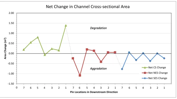
The average of the net changes experienced in all transects revealed that the two experimental

reaches displayed a largely aggradational trend in channel modification (NES = -0.7 % or -0.2 m2,

SES = -1.0 % or -0.2 m2) compared to the CS which had greater degradational channel characteristics

(+1.7 % or +0.5 m2) (Table 1). A definite pattern of upstream degradation becoming progressively more

aggradational downstream was visible when looking at the average changes from CS through SES in

100 150 200 250 300 350 400 450 500 550 600 650

0 5 10 15 20

El e vation (c m )

Distance from Left Bank Pin (m)

Control - Section 3

Pre Flood Post Flood

100 150 200 250 300 350 400 450 500 550 600 650

0 5 10 15 20

El e vation (c m )

Distance from Left Bank Pin (m)

Control - Section 1

100 150 200 250 300 350 400 450 500 550 600 650

0 5 10 15 20

El e vation (c m )

100 150 200 250 300 350 400 450 500 550 600 650

0 5 10 15 20

El e vation (c m )

Distance from Left Bank Pin (m)

Control - Section 6

Pre Flood Post Flood

100 150 200 250 300 350 400 450 500 550 600 650

0 5 10 15 20

El e vation (c m )

Distance from Left Bank Pin (m)

Control - Section 4

100 150 200 250 300 350 400 450 500 550 600 650

0 5 10 15 20

El e vation (c m )

Figure 3.1 – Control Site cross-sectional analysis

Cross-sectional plots of pre- and post-flood channels in the CS. The red, dashed line denotes the high flow mark used for the area calculation.

100 150 200 250 300 350 400 450 500 550 600 650

0 5 10 15 20

El

e

vation

(c

m

)

Distance from Left Bank Pin (m)

Control - Section 7

Pre Flood Post Flood

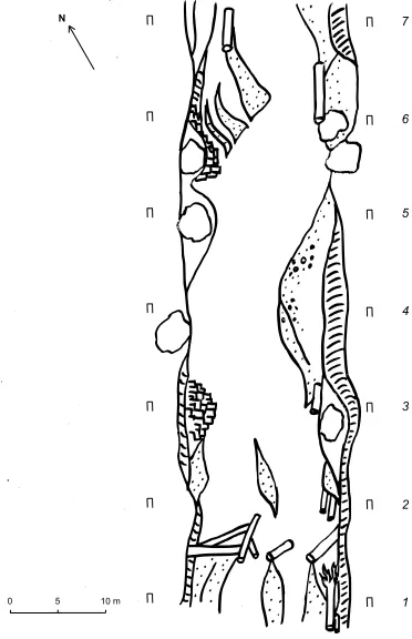
Figure 3.2 – Control Site sketch

50 100 150 200 250 300 350 400 450

0 5 10 15 20

El e vation (c m )

Distance from Left Bank Pin (m)

N Experimental - Section 3

Pre Flood Post Flood

50 100 150 200 250 300 350 400 450

0 5 10 15 20

El e vation (c m )

Distance from Left Bank Pin (m)

N Experimental - Section 1

50 100 150 200 250 300 350 400 450

0 5 10 15 20

El e vation (c m )

50 100 150 200 250 300 350 400 450

0 5 10 15 20

El e vation (c m )

Distance from Left Bank Pin (m)

N Experimental - Section 4

50 100 150 200 250 300 350 400 450

0 5 10 15 20

El e vation (c m )

Distance from Left Bank Pin (m)

N Experimental - Section 5

50 100 150 200 250 300 350 400 450

0 5 10 15 20

El e vation (c m )

Distance from Left Bank Pin (m)

N Experimental - Section 6

Figure 3.3 – North Experimental Site cross-sectional analysis

Cross-sectional plots of pre- and post-flood channels in the NES. The red, dashed line denotes the high flow mark used for the area calculation.

50 100 150 200 250 300 350 400 450

0 5 10 15 20

El

e

vation

(c

m

)

Distance from Left Bank Pin (m)

N Experimental - Section 7

Pre Flood Post Flood

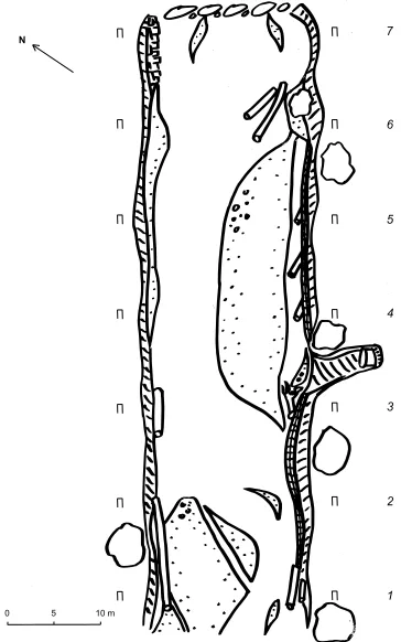
Figure 3.4 – North Experimental Site sketch

50 100 150 200 250 300 350 400 450

0 5 10 15 20

El e vation (c m )

Distance from Left Bank Pin (m)

S Experimental - Section 1

50 100 150 200 250 300 350 400 450

0 5 10 15 20

El e vation (c m )

Distance from Left Bank Pin (m)

S Experimental - Section 2

50 100 150 200 250 300 350 400 450

0 5 10 15 20

El e vation (c m )

Distance from Left Bank Pin (m)

S Experimental - Section 3

50 100 150 200 250 300 350 400 450

0 5 10 15 20

El e vation (c m )

Distance from Left Bank Pin (m)

S Experimental - Section 4

50 100 150 200 250 300 350 400 450

0 5 10 15 20

El e vation (c m )

Distance from Left Bank Pin (m)

S Experimental - Section 5

50 100 150 200 250 300 350 400 450

0 5 10 15 20

El e vation (c m )

Distance from Left Bank Pin (m)

S Experimental - Section 6

Figure 3.5 – South Experimental Site cross-sectional analysis

Cross-sectional plots of pre- and post-flood channels in the SES. The red, dashed line denotes the high flow mark used for the area calculation.

50 100 150 200 250 300 350 400 450

0 5 10 15 20

El

e

vation

(c

m

)

Distance from Left Bank Pin (m)

S Experimental - Section 7

Pre Flood Post Flood

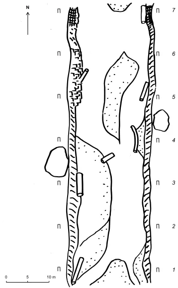
Figure 3.6 – South Experimental Site sketch

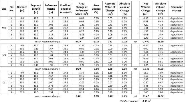
Table 1 – Results from the cross-sectional resurvey analysis

Changes in channel cross-sectional area and channel volume for the study reach representing the total amount of scour and fill per cross-section as positive and negative values respectively. The post-flood channel dimension for each transect was used as the baseline for area change calculations. For channel volumes each cross-section represents a segment of the channel length. Positive and negative values represent the total amount of sediment eroded and deposited respectively.

Site Pin

No. Distance (m) Segment Length (m) Reference Height (m) Pre-flood Channel Area (m2₎

Area Change at Reference Stage (m2)

Area Change (%) Absolute Value of Change

(m2)

Absolute Value of Change (%) Net Volume Change (m3)

Absolute Volume Change (m3)

Dominant Process

NES

1 0.0 10.0 2.18 26.0 0.05 0.2% 0.05 0.2% 0.55 0.55 degradation 2 10.0 9.20 2.16 26.2 0.05 0.2% 0.05 0.2% 0.48 0.48 degradation 3 18.3 10.0 2.01 25.6 -0.41 -1.6% 0.41 1.6% -4.12 4.12 aggradation 4 30.0 10.9 1.89 26.2 0.13 0.5% 0.13 0.5% 1.44 1.44 degradation 5 40.0 10.0 1.60 25.9 0.20 0.8% 0.20 0.8% 1.98 1.98 degradation 6 50.0 10.0 2.14 26.7 -1.09 -4.1% 1.09 4.1% -10.9 10.9 aggradation 7 60.0 10.0 2.20 25.1 -0.24 -1.0% 0.24 1.0% -2.41 2.41 aggradation

reach mean net change -0.19 -0.7% 0.31 1.2% net -13.00 21.90

SES

1 0.0 10.0 1.67 23.9 -0.24 -1.0% 0.24 1.0% -2.43 2.43 aggradation

2 10.0 9.10 1.67 23.6 0.00 0.0% 0.00 0.0% 0.00 0.00 -

3 18.2 10.0 1.76 24.1 -0.38 -1.6% 0.38 1.6% -3.76 3.76 aggradation

4 30.0 10.9 1.84 23.7 0.01 0.0% 0.01 0.0% 0.12 0.12 -

5 40.0 10.0 2.03 23.2 -0.33 -1.4% 0.33 1.4% -3.29 3.29 aggradation 6 50.0 9.40 2.09 23.8 0.05 0.2% 0.05 0.2% 0.51 0.51 degradation 7 58.7 9.40 1.95 22.9 -0.77 -3.4% 0.77 3.4% -7.25 7.25 aggradation

reach mean net change -0.24 -1.0% 0.26 1.1% net -16.10 17.36

CS

1 0.0 10.0 2.43 27.3 1.39 5.1% 1.39 5.1% 13.9 13.9 degradation 2 10.0 10.0 2.57 28.8 0.16 0.5% 0.16 0.5% 1.55 1.55 degradation 3 20.0 10.0 2.55 27.6 0.23 0.8% 0.23 0.8% 2.33 2.33 degradation 4 30.0 10.0 2.60 27.6 -0.07 -0.2% 0.07 0.2% -0.67 0.67 aggradation 5 40.0 10.5 2.73 27.4 0.80 2.9% 0.80 2.9% 8.41 8.41 degradation 6 51.0 11.0 2.47 28.8 0.54 1.9% 0.54 1.9% 5.99 5.99 degradation 7 62.0 10.5 2.54 27.6 0.19 0.7% 0.19 0.7% 2.00 2.00 degradation

reach mean net change 0.46 1.7% 0.48 1.7% net 33.47 34.82

-1.50 -1.00 -0.50 0.00 0.50 1.00 1.50 2.00

0 5 10 15 20

A

re

a C

h

an

ge

(

m

2)

Pin Locations in Downstream Direction

Net Change in Channel Cross-sectional Area

Net CS Change

Net NES Change

Net SES Change

7 6 5 4 3 2 1 7 6 5 4 3 2 1 7 6 5 4 3 2 1

Degradation

Aggradation

Figure 3.7 – Plot of channel area alterations

-15.00 -10.00 -5.00 0.00 5.00 10.00 15.00 20.00

1 2 3 4 5 6 7

N

e

t

Vo

lu

m

e

tr

ic

Ch

an

ge

(

m

3)

Site Pin Number

Net Change in Cross-sectional Segment Volumes

CS Net Volume

SES Net Volume

NES Net Volume

Scour

Fill

Figure 3.8 – Plot of volumetric channel changes per cross-sectional segment

Aggradation in the SES was largely exhibited by lateral channel bar development in the upper

reaches (pin 5-7) and to some degree in the lower reach (pin 1). An interesting feature in this site was

the development of point bar along the right bank through transects of pin 3 to pin 4 (Figure 3.5 and

Figure 3.6), as sediment from the mid-channel was generally eroded. In the NES aggradation was

dominant mainly because of deposition in the upper reaches (pin 6 and 7) and occurrence of a log in mid

reach (pin 3). The overall net change indicated channel narrowing, but excluding these above mentioned

features would have made this channel degradational (Table 1). The pin 7 transect was essentially taken

across a scour pool, where an influx of sand developed left and right bank point bars. The rock weir

above this site was redirecting the flow towards the left bank, which although not measured in this

study, had been severely undercut and eroded in the past. A probable legacy of this was that a

prominent lower bank aggradation was taking place on the right banks along the pin 6 transect (Figure

3.6). In the remainder of the site there was a degree of thalweg migration as the channel meandered

filling in previous thalweg locations and redistributing channel bar sediments (pin 2-6).

For the most part the CS experienced predominant channel erosion over the duration of the

study period. As with the NES, there was a migration of the thalweg channel as meandering tended to

scour new low-flow channels and degrade exiting channel bars (Figure 3.1). The resurvey of these

channel banks along precisely the same transect line was complicated by the presence of tree roots,

overhanging banks, and persistent vegetation cover. The comparative measurements of changes in bank

dimension were therefore adjusted in the spreadsheet calculations to compensate for any anomalous

bank adjustments. Bank aggradation did however take place along the left bank above a log in the

channel along the pin 6 transect of and on the right bank along the pin 2 transect. The largest erosion

took place below a channel debris constriction upstream of the pin 1 transect causing the removal of

The sum of the absolute changes for all transects in each reach, demonstrated that the total

amount of both scour and fill relating to the alteration in each reach was different (Table 1). Statistical

results from comparing these changes between individual sites were not considered significant (p > 0.05

for α = 0.05 using Mann-Whitney test and two-tailed t-test) (Table C). When all three reaches were

compared, the CS represented the largest amount of absolute change (1.7 % see Table 1), the NES

experienced a moderate amount of change (1.2 %) and the SES exhibited the least amount of change

(1.1 %). Average changes in the CS almost culminated to as much as the average changes of both

experimental sites together (Table 1), but this does not directly indicate the CS as the sediment source.

As demonstrated by the NES and SES channels, the measure of absolute change lends a greater

understanding of the true amount of actual bed movement through each site and although the SES

demonstrated the greatest degree of aggradation, the NES experienced considerably more bed mobility.

These changes may also be translated into the relative amount of instability which exists in this channel

(see Schoonover et al. (2007)).

Channel shape also warranted inspection following resurveying of channel sections, and in many

cases these shapes could be attributed to possible stages according to the channel evolution model

(CEM) for incising rivers (Simon, 1994). In this model, the channel morphology of a degraded stream

progresses through six stages as it adjusts to imposed disturbances such as urbanization (Simon, 1989;

Doyle and Shields, 2000; Niezgoda and Johnson, 2005). Stage I includes the premodified, unaltered

channel form and as construction commences, the watershed becomes a significant sediment source as

stream channels become channelized during Stage II. As the watershed becomes developed and

impervious surface cover causes increased runoff during precipitation events, stream channels become

incised (Stage III) and consequent bank failures cause channels to widen (Stage IV). The channel bed

begins to aggrade with continued widening in Stage V, and channels ultimately reach a quasi-equilibrium

Not enough time had accumulated for any of the channel dimensions to change significantly,

especially since bed erosion and deposition was more prevalent than bank involvement and so channels

were thought to represent their current stage in evolution. The CS had an entrenched, trapezoidal shape

confined by its steeply incised banks and resembled a Stage III or IV. Riparian vegetation was set very

high relative to the flow line and the upper right banks were frequently vertical in this channel. The NES

also appeared trapezoidal in shape but bank angles were gentler compared to the CS banks with fallen

riparian vegetation becoming established on the lower bank line (Figure 3.3 and Figure 3.4). This site

was subjected predominantly to degradation of the channel bed but the magnitude of deposition

concurrently occurring classified this site as aggradational and therefore qualifying it as a Stage V

channel. The lower and characteristically aggradational SES had low bank heights, had more rounded

channel dimensions with a pronounced convex bank shape particularly for the right banks. The SES,

according to the CEM, would likely represent a late Stage V channel.

3.2 Sediment Volume

The total volume of sediment moving through each reach was estimated using the cumulative or

net change in channel area as discussed above. Between the three sites there was a visible

aggradational development in the downstream direction culminating in the SES channel (Figure 3.8). The

total change in volume for the study was 4.4 m3 of bed-material, which was representative of a net

degradation (Table 1). While the SES had experienced one less effective flow event, the results albeit

indicated that more loss of bed-material could be accounted for in the CS than could be balanced as

influx into both study sites together. However, a sediment budget approach cannot be considered

absolute in this instance because the surveyed reaches are not directly connected and the fate of

sediments can only be loosely inferred. This implies that sediments are additionally stored in reaches

balance of scour and fill in all three reaches. Cumulative volumes of 13.0 m3 and 16.1 m3 were being

deposited in the NES and SES channels respectively and the CS experienced a net removal of 33.5 m3 of

bed-material from its channel. This also makes the latter site with the most net change as would be

expected from the section results. Because the segment volumes were calculated using the

cross-section areas, the patterns observed in the area change plots are repeated for the volumetric trends

(Figure 3.7 and Figure 3.8). The NES showed variations between degradation and aggradation, and

although it experienced a lower amount of aggradation than the SES, it generally shows a larger

absolute change in volume compared to that site (NES = 21.9 m3 versus SES = 17.4 m3).

Table 2 - Channel sediment volume densities

Bulk density estimates calculated using channel segment volumetric changes (method based on densities used by Fraley et al. (2009)).

grain size density

(g/cm3) kg/m

3 average sample

representation

clay/silt 1.3 1330 0.1%

fine sand 1.5 1460 6.6%

med/coarse sand 1.7 1720 86.4%

fine gravel 2.3 2250 6.8%

medium gravel 2.4 2400 0.2%

CS NES SES

sediment volume (m3) 33.5 -13.0 -16.1

sediment mass (t) 58.3 -22.6 -28.0

3.3 Grain-size Analysis

3.3.1 Bed-material Subsurface

The grain size distribution of bed-material samples for all three sites were generally uni-modal,

moderately well to poorly sorted compositions of medium to coarse sand and fine gravel with typical D50

values ranging from 0.43 mm to 1.03 mm. Overall the resulting changes in grain size distributions within

and between sites during the study period were not deemed statistically significant by Mann-Whitney

tests or two-tailed t-tests (p > 0.05 for α = 0.05) (Table C). For this study it was expected that bed

sediments would be significantly different in the mitigation site compared to upstream locations due to

observed bank erosion caused by bank engineering. The similarity between pre- and post-flood sample

distributions points towards a common sediment source further upstream. Channel processes at work in

the upper Snapfinger Creek watershed are still providing large sources of sand-sized bed load material,

which is moving for the most part downstream as pulses with each high-flow event in the form of

bed-forms (Knighton, 1998). The high proportion of sand in the channel bed implies that this material is likely

frequently mobilized (Schoonover et al., 2007). Another expected result was that the sites in the lower

reaches would experience a bed fining as upstream channels became more coarse grained. The results

show no indication of this because the channel morphology controls in this reach are largely affected by

bed processes such as the reworking of sand in the form of scour and fill.

All three channels had median grain sizes which did not shift significantly from that of coarse

sand, but minor trends in distributions were noticeable. Pre- and post-flood grain-size distributions for

the NES remained largely identical even though the latter was a larger sample quantity (Figure 3.9 and

Figure1A) with median D50 grain sizes not changing from around 0.7 mm (0.5 ɸ). The bed-material of the

SES was not as univariant as it generally coarsened from a D50 of 0.5 mm to 0.7 mm. The reverse could

be said for the CS, whose bed generally became less coarse as D50 went from 0.7 mm to 0.5 mm. It is