www.hydrol-earth-syst-sci.net/17/341/2013/ doi:10.5194/hess-17-341-2013
© Author(s) 2013. CC Attribution 3.0 License.
Earth System
Sciences
Parameterizing sub-surface drainage with geology to improve
modeling streamflow responses to climate in data limited
environments
C. L. Tague1, J. S. Choate1, and G. Grant2 1University of California, Santa Barbara, USA
2USDA Forest Service, Pacific Northwest Research Station, Corvallis, Oregon, USA
Correspondence to: C. L. Tague ([email protected])
Received: 7 June 2012 – Published in Hydrol. Earth Syst. Sci. Discuss.: 18 July 2012 Revised: 30 November 2012 – Accepted: 12 December 2012 – Published: 29 January 2013
Abstract. Hydrologic models are one of the core tools used to project how water resources may change under a warming climate. These models are typically applied over a range of scales, from headwater streams to higher order rivers, and for a variety of purposes, such as evaluating changes to aquatic habitat or reservoir operation. Most hydrologic models re-quire streamflow data to calibrate subsurface drainage pa-rameters. In many cases, long-term gage records may not be available for calibration, particularly when assessments are focused on low-order stream reaches. Consequently, hydro-logic modeling of climate change impacts is often performed in the absence of sufficient data to fully parameterize these hydrologic models. In this paper, we assess a geologic-based strategy for assigning drainage parameters. We examine the performance of this modeling strategy for the McKenzie River watershed in the US Oregon Cascades, a region where previous work has demonstrated sharp contrasts in hydrology based primarily on geological differences between the High and Western Cascades. Based on calibration and verification using existing streamflow data, we demonstrate that: (1) a set of streams ranging from 1st to 3rd order within the West-ern Cascade geologic region can share the same drainage pa-rameter set, while (2) streams from the High Cascade ge-ologic region require a different parameter set. Further, we show that a watershed comprised of a mixture of High and Western Cascade geologies can be modeled without addi-tional calibration by transferring parameters from these dis-tinctive High and Western Cascade end-member parameter sets. More generally, we show that by defining a set of end-member parameters that reflect different geologic classes, we
can more efficiently apply a hydrologic model over a geo-logically complex landscape and resolve geo-climatic differ-ences in how different watersheds are likely to respond to simple warming scenarios.
1 Introduction
studies often assume that parameters used for a larger gaged watershed can be consistently applied to smaller sub-watersheds, or that parameters from neighboring watersheds can be used. Calibration based on gauges from a larger or-der watershed however, does not necessarily apply to the di-versity of lower order streams within that watershed. Simi-larly, parameter transfer from neighboring watersheds may not be appropriate. In this paper we present a relatively sim-ple strategy for parameter transfer based on geologic similar-ity. We hypothesize that for regions with sharp geologic con-trasts, we can develop end-members parameter sets based on geologic classification that can be used to parameterize hy-drologic models across a range of scales without additional calibration.
Parameter transfer schemes, where parameters are as-signed based on some readily measured watershed charac-teristics, offer one approach for assigning drainage param-eters when estimates of streamflow across a range of wa-tersheds are needed. In fact, when drainage parameters are assigned based on calibration of a larger watershed, stream-flow estimates for nested subcatchments implicitly transfer parameters and assume similarity of those parameters across the larger watershed. Studies on parameter transfer have used watershed size, elevation, and vegetation as a basis for trans-ferring parameters between watersheds with varying degrees of success (e.g., van der Linden and Woo, 2003; Wagener and Wheater, 2006). These studies focus on overall model performance using different parameter schemes, but do not explicitly address implications for estimating climate change impacts. Evaluation of parameter transfer schemes, calibra-tion approaches, and model performance in general should ultimately reflect the context in which the model is being used. How good is good enough depends on the modeling goal.
Drawing on an example from the snow-dominated moun-tains of the Cascades in Western Oregon, here we evaluate parameter transfer approaches in the context of assessing cli-mate change impacts on streamflow. Our broader focus is on the analysis of drainage parameter transfer within the frame-work of snowmelt-dominated watersheds in the mountainous Western US, and the use of hydrologic models to estimate how streamflow seasonality in these watersheds will respond to a warming climate. The hydrology of mountain regions throughout the globe is expected to be highly vulnerable to a warming climate (Barnett et al., 2005). In snow-dominated regions, warmer temperatures can reduce the amount of pre-cipitation falling as snow and lead to earlier snowmelt, partic-ularly at elevations where the majority of precipitation falls near 0◦C (Nolin and Daly, 2006). These changes in snow dynamics shift the timing of seasonal hydrographs, result-ing in increased flow in winter and reductions durresult-ing sprresult-ing and summer (Knowles and Cyan, 2002; Barnett et al., 2005; Stewart et al., 2005). Process-based hydrologic models are one of the core tools used to project how water resources in
these systems are likely to respond to climate variability and change.
In this study, we investigate drainage parameter variation and its implication for hydrologic model-based estimates of seasonal streamflow responses to climate warming within the McKenzie River watershed in Western Oregon. Our ap-proach applies a process-based hydro-ecological model, the Regional Hydro-Ecologic Simulation System (RHESSys), and focuses on the estimation of seasonal streamflow re-sponse to climate change at multiple spatial scales. We pro-pose an end-member mixing approach to parameter trans-fer, where end-member sub-watersheds are defined based on geologic classification and used to estimate spatial pat-terns of drainage parameters. We then examine the utility of this parameter transfer strategy within the context of pre-dicting inter-annual variation in seasonal streamflow patterns and streamflow response to climate warming in the snow-dominated watersheds of the Oregon Cascades.
2 Background
spatial patterns of snow accumulation and melt change, and (2) how those changes in input translate into changes in streamflow behavior (Fig. 1). The latter is primarily con-trolled by subsurface drainage characteristics. Changes in evapotranspiration fluxes are a 3rd factor and can become increasingly important when climate change substantially al-ters vegetation structure through disturbances. A significant research focus in the Western US has been on improving models of snow accumulation and melt, as well as spatially explicit estimates of climate forcing functions (Daly et al., 1994). Translating these effects into streamflow change how-ever, also requires adequate estimates of subsurface drainage characteristics. Our previous work has demonstrated that within the McKenzie, geologically mediated spatial differ-ences in subsurface drainage characteristics can be a 1st or-der control on spatial patterns of streamflow response to warming (Tague and Grant, 2009). Subsurface drainage char-acteristics reflect both topography, which is relatively easy to parameterize given the widespread availability of DEMs, and effective subsurface conductivity of watersheds, where con-ductivity is a complex product of matric- and macropore flow rates and their distribution (Troch et al., 2009). In most hy-drologic modeling studies, parameters associated with effec-tive conductivity, such as hydraulic conductivity and macro-pore distributions, are calibrated or assumed to be spatially uniform. Given that subsurface drainage properties evolve through landscape evolutionary processes, one might expect that these parameters would vary across geological classi-fication (Jefferson et al., 2006, 2010). Empirical studies and models based on streamflow patterns in the Oregon Cascades support this assertion (Tague and Grant, 2004, 2009).
[image:3.595.326.525.59.304.2]Within the McKenzie River watershed, sharp geologic contrasts exist between two largely contiguous geologic provinces: (1) the Plio-Pleistocene High Cascades (HC) to the east, and (2) the primarily Miocene Western Cascades (WC) to the west (Sherrod and Smith, 2000). Elevations range from 400 to 1800 m in the WC and from 1500 m to over 3400 m at the summits of the large stratovolcanoes in the HC. Although the HC region has the highest elevations, much of the landscape is a broad constructional platform with rela-tively low relief; the WC is much steeper and more dissected. Young basaltic lava flows dominate the HC province while older lava flows and volcaniclastic rocks dominate the WC province. These distinctions drive hydrologic flowpath dif-ferences and residence times (Jefferson et al., 2006). The young lava flows in the HC have exceptionally high perme-ability with high vertical hydraulic conductivity, resulting in a greater portion of deep groundwater flow and large vol-ume spring discharges. The high vertical conductivity allows recharge to quickly drain through the shallow and undevel-oped soils and intersect large deep aquifers, where residence times can be on the scale of years or decades (Jefferson et al., 2006). In the WC, greater drainage efficiencies due to steep lateral hydraulic gradients, shallow bedrock, and clay aquitards confine recharge to the shallow subsurface region,
Fig. 1. Landscape responses to precipitation inputs – as a series of filters (Tague and Grant, 2009).
producing quicker transfer of recharge to streamflow (Tague and Grant, 2004). These differences in flowpaths, and there-fore subsurface residence times, lead to distinctively differ-ent hydrologic regimes, characterized by higher baseflows, slower recessions, and muted flood peaks in HC watersheds (Tague and Grant, 2009). During winter storm and early spring snowmelt peaks, recharge in WC regions quickly en-ters streams, contributing a greater portion to flow than in HC regions. During summer periods, months after the last sub-stantial precipitation has fallen, the groundwater storage in WC systems is largely depleted (Jefferson et al., 2006), and the pattern reverses as the majority of flow in the McKenzie originates from slow-draining HC aquifers (Tague and Grant, 2004).
warming impacts on streamflow seasonality respond to these strategies for assigning drainage parameters.
3 Methods
RHESSys (Tague and Band, 2004) is a physically based, spa-tially distributed, hierarchical daily time-step model that cou-ples watershed hydrology, vegetation growth, and soil bio-geochemical cycling processes. It models both vertical and lateral hydrologic processes. As a spatial model, RHESSys discretizes the landscape into a hierarchy of spatial objects including: watersheds; hillslopes, which drain to either side of a stream reach; zones, which are areas of similar meteoro-logical forcing within hillslopes; and finally patches, which are typically 30 to 90 m scale modeling units. Most verti-cal processing of hydrologic and carbon cycling processes is done at the patch scale; while shallow subsurface moisture redistribution occurs between patches at the hillslope scale, and a deeper groundwater store is also modeled at the hill-slope scale. The shallow subsurface flow model considers four layers: (1) a surface detention store, (2) rooting zone, (3) unsaturated store, and 4) saturated zone store, and routes this surface and shallow subsurface water laterally between model units (30–120 m patches) based on topography and soil drainage parameters. Transpiration of infiltrated water, as well as evaporation of water from interception, litter, and soil is estimated using the Penman-Monteith approach. Deeper groundwater flow of water that bypasses the shallow sub-surface flow system is modeled at a coarser hillslope scale (unit draining either side of a stream reach) using a linear storage-discharge relationship. RHESSys has been applied in a number of mountain catchments in the Western US (Baron et al., 2000; Tague and Grant, 2009), as well as mountain-ous catchments in Europe (Zierl et al., 2006), and evaluated against respective catchment observed streamflow, snow, car-bon and moisture flux data. The model’s physical treatment of rain and snow partitioning, snow melt, shallow and deep groundwater flow, and evapotranspiration make it a suitable tool for studying the impacts of global change on mountain hydrology. Details of RHESSys process representation are summarized in Tague and Band (2004).
RHESSys model inputs consist of meteorological time se-ries data and GIS-based inputs of topography, soils, land use, and land cover. For simplicity, we use data from a single me-teorologic station as input. While this paper focuses on the role of subsurface drainage uncertainty, another key chal-lenge in estimating streamflow in mountain environments is distributing meteorological and, in particular, precipita-tion data. For this study, we account for spatial variaprecipita-tion in precipitation using a single meteorological station com-bined with widely available PRISM mean annual precipita-tion grids (Day et al., 1994) to derive spatially variable esti-mates for daily precipitation data. For temperature, we also use the same meteorological station and adjust temperature
input data based on standard elevational lapse rates. While additional meteorological stations are located within the wa-tershed, long-term records at multiple meteorological sta-tions are often unavailable. In contrast, approaches for inter-polating climate data such as PRISM are available for wide geographic areas. Here we test how well streamflow char-acteristics can be predicted for different watersheds using commonly available data sets. Other GIS data sets, such as soils, land cover, and elevation, are obtained from the Ore-gon Geospatial Data Clearinghouse.
There are six hydrologic parameters that can be calibrated in RHESSys. Two parameters control soil transmissivity:K
(m day−1), the saturated hydraulic conductivity at the sur-face; andm(meters), the exponential decay of saturated con-ductivity with depth; such that:
K(z)=exp(−zρ/m). (1) Herezis depth (m) below the surface andρis porosity. Two parameters control soil moisture holding capacity: po – pore size index; and pa (meters of water), soil water potential at air entry; and two parameters control deeper ground-water drainage: gw1, the percentage of subsurface water that enters a deep groundwater storage, bypassing shallow subsurface flowpaths and rooting zone storage; and gw2 (% day−1), the rate of drainage from the deep groundwater storage. The last two parameters are only included in parameterization if this deeper ground-water store is needed, i.e., for watersheds with HC geology (Tague and Grant, 2004). Where deep ground-water is not present, a simpler representation of subsurface drainage is obtained by setting gw1 to 0, thus using only a shallow subsurface flow representation in the watershed.
The gw1 and gw2 parameters are used to characterize the deeper ground water systems that are well below the biolog-ical active soil and rooting zone. The other four parameters (po, pa,m,K) reflect soil characteristics and shallow sub-surface flowpaths. We hypothesize that the younger, deeper groundwater dominated HC region will lead to higher values of gw1. We also note, however, that soil water-holding capac-ity (parameters po and pa) and shallow subsurface drainage (mandK) are also likely to depend on the time taken for soil development. Western Cascade soils are derived from bedrock that has weathered in place for up to 30 million years, over which time a wide range of clay species have de-veloped forming impervious layers and aquacludes. Infiltra-tion rates are high with abundant residual stones and clasts (Dyrness, 1969), and soils are shallow due to mass wasting and creep. In contrast, HC soils are much younger (less than seven million years) and typically lack abundant clays and corresponding impermeable layers. They also occupy much lower gradient portions of the landscape, meaning that hy-draulic gradients are gentler.
Table 1. Watershed characteristics.
Watershed Abbreviation Drainage Elevation Geology
(WS) (km2) (m)
Budworm Creek BUD 7.77 (54.5) 619–1626 WC
Lookout Creek HJA 62.4 428–1620 WC
Mack Creek MACK 5.8 758–1610 WC
Watershed 2 W2 0.60 548–1070 WC
Watershed 8 W8 0.22 993–1170 WC
Clearlake CLR 239.3 924–2019 HC
Horse Creek HORSE 387.5 439–3152 HC
Southfork SF 538.7 530–2044 36 % WC;
64 % HC
(CLR) and Horse Creek near McKenzie Bridge (HORSE). The five WC watersheds are Budworm Creek near Belknap Springs (BUD) and Lookout Creek (HJA), along with three sub-watersheds within the Lookout Creek drainage (MACK Creek, W2, and W8). The number of HC watersheds con-sidered was limited by the small number of gaged sheds draining predominately HC geology. All seven water-sheds were calibrated for two water years, following a sin-gle year of spin-up. All watersheds were run across the same 1500 randomly generated parameter sets by sampling from a uniform random distribution within realistic ranges for each of the six parameters. For 300 of the 1500 parameter sets, we set gw1 equal to 0 in order to run a simpler (and more parsimonious) model. Realistic ranges for each parameter were established based on RHESSys parameter libraries. We used two performance metrics, the Nash–Sutcliffe Efficiency (NSE) and the NSE of log-transformed flow (NSElog), to evaluate the parameter sets. The Nash–Sutcliffe Efficiency is a commonly used metric for evaluating streamflow pre-dictions from hydrologic models. Because streamflow in this region has a high dynamic range (high winter peaks and low summer flows), we add the NSE of log-transformed flows to test whether the model can capture recession and summer flow behavior as well as storm flows.
[image:5.595.50.287.81.195.2]For each watershed, we compared the number of accept-able parameter sets as well as sensitivity of model perfor-mance to each parameter. We examine how acceptable pa-rameter values differ between HC watersheds and WC wa-tersheds relative to comparisons of acceptable parameter sets within WC watersheds alone. The parameter sets are con-sidered acceptable if the NSElog value>0.5; we also con-sider a more stringent criterion >0.8. We then define our generalized HC parameter sets as those that are acceptable for both of the two HC watersheds and our generalized WC parameter sets as those that are acceptable for all five WC watersheds. To test model performance, we selected four cal-ibrated parameter sets from the generally acceptable data set and ran RHESSys for all years for which streamflow is avail-able (>25 water years for most watersheds). Parameter sets were selected to cross a range of different parameter values,
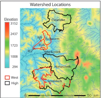
Fig. 2. Map showing study watersheds (listed in Table 1) and geo-logic classification.
but all gave model results within the acceptable performance criteria.
To assess the use of geologic classification as a method for assigning hydrologic parameters, we apply RHESSys to the South Fork McKenzie (SF) watershed (comprised of both HC and WC geology; Table 1, Fig. 2). We use an end-member mixing approach, where drainage parameters within SF are assigned based on drainage parameters for “pure” WC and HC watersheds. In other words, parameters are varied spatially according to HC/WC geologic classification within the SF watershed. The pure “WC” and “HC” parameters are the generally acceptable drainage parameters from the calibrations of HC and WC described above. Thus, for the portion of SF with HC geology (approximately 64 % of the drainage area), we use parameter sets that had acceptable per-formance from the CLR and HORSE calibrations. For the WC portion (36 %), we use parameter sets that had accept-able performance across all five WC watersheds.
0.1 0.2 0.5 1.0 2.0 5.0 10.0
0.0
0.2
0.4
0.6
0.8
1.0
m
Cum
ulativ
e NSElog
HORSE CLR BUD HJA MACK W2 W8 All Pars
0 50 100 150 200 250 300
0.0
0.2
0.4
0.6
0.8
1.0
K
0.5 1.0 1.5 2.0
0.0
0.2
0.4
0.6
0.8
1.0
Air entry Pressure
Cum
ulativ
e NSElog
0.5 1.0 1.5 2.0
0.0
0.2
0.4
0.6
0.8
1.0
Pore Size Index
Cum
ulativ
e NSElog
0.0 0.1 0.2 0.3 0.4
0.0
0.2
0.4
0.6
0.8
1.0
Ground Water 1
Cum
ulativ
e NSElog
0.0 0.2 0.4 0.6 0.8 1.0
0.0
0.2
0.4
0.6
0.8
1.0
Ground Water 2
Cum
ulativ
e NSElog
Cum
ulativ
e NSE log Cum
ulativ
[image:6.595.129.467.64.302.2]e NSE log
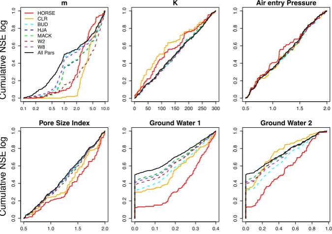
Fig. 3. Cumulative distribution of performance across parameter sets. The y-axis gives the cumulative probability of the performance measure (or parameter distribution). The x-axis gives the value of the parameter. Solid black line shows the original parameter distribution; colored lines show distribution of performance by parameter value for each watershed. Departures from the black line show preference for particular parameter values.
simulate the response of SF and other watersheds to both 2 and 4◦C warming scenarios (using one of the best
perform-ing parameter sets), and assess whether predicted changes are small or large relative to error in predicting historic stream-flow response to inter-annual climate variability. We apply a uniform temperature increase to historic meteorologic forc-ing data to generate the warmforc-ing scenarios. Predicted future warming scenarios in the PNW range between one and eight degrees (Mote and Salathe Jr., 2010). We acknowledge that a uniform warming scenario is simplistic and actual climate warming will be more temporally complex; we use it here, however, to assess the sensitivity of modeled streamflow to changes in temperature, given different assumptions about drainage parameters.
4 Results
Figure 3 illustrates the cumulative performance across pa-rameter values for each of our six calibration papa-rameters within each of the seven calibration watersheds. Following Thorndahl et al. (2008), we examine model sensitivity to spe-cific parameters by comparing this cumulative performance distribution with the cumulative distribution of parameter values. Calibration preference (or improved performance) for particular parameter values is demonstrated by a shift of the cumulative distribution of NSE or NSElog for that parame-ter relative to its cumulative distribution within the calibra-tion set (shown in Fig. 3 as a solid black line – this can be
interpreted as the reference distribution). Generally, depar-tures above the reference distribution indicate preference for parameter values in that range and vice-versa. Results were similar using the NSE performance metric so only NSElog results are shown. The greatest difference in acceptable pa-rameter distributions occurs between HC and WC sites; this difference is present for all parameters. Relative to the WC watersheds, the HC watershed CLR shows improved per-formance for higher values of gw1, lower values of gw2, higher values ofm, and lower values of K. This set of pa-rameters for a HC watershed reflect a slower draining system with greater proportions of infiltrated water connecting to a deeper groundwater reservoir. The HC watersheds also show a slightly different responses to air entry pressure (pa) and pore size index (po). All sites show a strong sensitivity tom
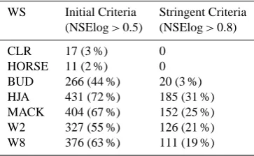
Table 2. Number of acceptable parameters sets for each watershed.
WS Initial Criteria Stringent Criteria (NSElog>0.5) (NSElog>0.8)
CLR 17 (3 %) 0
HORSE 11 (2 %) 0
BUD 266 (44 %) 20 (3 %)
HJA 431 (72 %) 185 (31 %)
MACK 404 (67 %) 152 (25 %)
W2 327 (55 %) 126 (21 %)
W8 376 (63 %) 111 (19 %)
et al., 2005). Improved performance for WC watersheds oc-curred with lower values of mrelative to HC watersheds. Lower values ofmdenote a steeper decline in hydraulic con-ductivity with depth, and are consistent with shallower hy-drologically active soils. This result is consistent with the more well-developed clay and bedrock confining layers as-sociated with the older WC geology.
Table 2 summarizes the number of acceptable parame-ter sets for each waparame-tershed. The waparame-tersheds differ in parame-terms of the percentage of parameter sets that achieved an ac-ceptable level of performance, where acac-ceptable was de-fined as NSElog>0.5. HJA had the highest (72 %) number of parameters that achieved acceptable performance, while HORSE had the lowest (2 %). There were 173 parameter sets that were acceptable for all WC sites (10 % of parameters, based on NSElog>0.5 criteria). None of the parameter sets that achieved acceptable performance for the WC sites also achieved acceptable performance for the HC sites. In other words, the set of acceptable parameters for the WC sites were mutually exclusive from those for the HC sites. Within the WC sites, however, there was substantial, although not com-plete, overlap of acceptable parameter sets.
There was some variation in overall performance in the calibration period between different sites. In general, sites with a larger number of acceptable parameters had higher overall performance. To try to further constrain parameter values, we consider a more stringent criteria, defined as NSElog >0.8 (Table 2). Using these more stringent crite-ria, there remain 17 parameter sets that are acceptable across BUD, HJA, MACK, and W8 sites. However, W2 parameter sets do not overlap with the other sites if these more strin-gent criteria are used. This difference in W2 performance re-flects its differing sensitivity to themparameter as discussed above.
[image:7.595.311.547.93.206.2]There are parameter sets that have gw1 set to 0 within those that are acceptable for BUD, HJA, MACK, and W8 using these more stringent criteria. We consider these sets to be preferable, given that they result in a simpler (more parsi-monious) model because the deeper groundwater store is not used. It is worth noting that none of the acceptable parameter
Table 3. Example of an acceptable parameter set across common geologic watersheds.
WS M K pa po gw2 gw2
(m) (m day−1) (m) (dim) (0–1) (0–1)
CLR 5.1 34 0.9 1.6 0.3 0.6
HORSE 5.1 34 0.9 1.6 0.3 0.6
BUD 0.8 58 1.8 1.1 0 0
HJA 0.8 58 1.8 1.1 0 0
MACK 0.8 58 1.8 1.1 0 0
W8 0.8 58 1.8 1.1 0 0
W2 1.8 249 1.8 1.3 0.2 0.6
sets for the HC watershed have gw1 set to 0. Thus, for the HC watersheds, a deeper groundwater store must be included.
For validation, we randomly selected four parameter sets from those that were considered acceptable for the WC sites and then for the HC sites, respectively, using the more strin-gent selection criteria. We argue that any of these parameter sets could be selected as the “best” parameter set in a calibra-tion process, depending on the criteria used or the calibracalibra-tion period. We examine results from four parameters within the acceptable set to ensure that our results are not overly de-pendent on which “acceptable” parameter set is chosen. For BUD, HJA, MACK, and W8, we use parameter sets that met the more stringent criteria for all sites, and two that did not in-clude a deeper groundwater store (gw1 was set to 0). We con-sider these parameters to be examples of WC end-member parameter sets. We exclude W2 calibrations from developing the end-member WC parameter set because of their deviation from other WC watersheds and the evidence of observation error as the cause of this difference as noted above. For W2 simulations itself, however, we use parameters that met the more stringent criteria for W2 and the initial criteria for all WC sites. For HORSE and CLR, we randomly selected four parameter sets that met the more stringent criteria for both of those sites, and consider these parameters to be examples of HC end-member parameters. Table 3 summarizes one of the parameter sets selected.
Table 4. Model performance across four chosen parameters.
WS Calibration Evaluation Evaluation
(WY 1999–2000) (longest period) (WY 1980–1986)
NSElog NSE NSElog NSE Eval. period NSElog NSE
CLR .51–.67 .30–.68 .61–.68 .55–.56 WY 70–06 .54–.62 .50–.53
HORSE .50–.62 .46–.65 .52–.59 .40–.48 WY 62–69 NA NA
BUD .80–.83 .62–.68 .68–.75 .40–.45 WY 79–86 .67–.74 .40–.44
HJA .82–.91 .72–.82 .68–.82 .47–.60 WY 58–05 .70–.80 .49–.62
MACK .85–.91 .60–.70 .68–.76 .41–.49 WY 80–06 .56–.69 .40–.53
W2 .83–.91 .51–.61 .69–.75 .36–.44 WY 58–06 .66–.74 .31–.43
W8 .88–.89 .60–.66 .74–.75 .35–.37 WY 64–05 .69–.72 .39–.46
SF NA NA .75–.80 .58–.66 WY 58–88 .68–.75 .59–.69
from the meteorologic station, and thus are most susceptible to errors in spatial interpolation of precipitation.
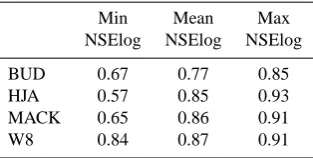
To demonstrate the effectiveness of end-member param-eters for the WC region, we compute the range of NSElog values obtained for full simulation period for each WC wa-tershed using only the set of parameters that were accept-able for all other WC watersheds (Taccept-able 5). We exclude W2 from this analysis. Essentially, these show the range of per-formance that would have been obtained for that watershed if parameters were based on acceptable WC end-member pa-rameter sets, rather than calibration of that particular water-shed. Acceptable end-member parameters were based on cal-ibration of the other WC watersheds. Results show good per-formance for all WC watersheds, including the nested wa-tersheds within the HJA (W8 and MACK) as well as the neighboring watershed (BUD). We could not repeat this ex-periment for HC because we were limited to only two end-member HC watersheds. However, generalization of HC pa-rameters is supported by results from the mixed-geology SF watershed, as discussed below.
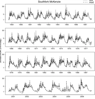
Streamflow predictions for SF, resulting from a set of pa-rameters transferred using the geologic end-member mix-ing described above, show good correspondence between observed and modeled flows (Fig. 4). Based on our initial model implementation using this approach, streamflow pre-dictions were consistently 20 % lower than observed stream-flow across all parameter sets. The long-term bias of 20 % in total streamflow likely reflects a bias in input rather than drainage parameters, which tend to influence the hydrograph shape. Error in precipitation input estimates is not surpris-ing given that precipitation inputs are based on a meteoro-logic station more than 27 km from SF. Although PRISM was also used to scale precipitation from the meteorologic site, PRISM grids are also relatively coarse (200 m). Since the focus of this paper is on drainage parameters, we simply applied a 20 % increase in precipitation input to the model to account for the difference. We note, however, that the neces-sity of post-hoc precipitation adjustment illustrates the sensi-tivity to precipitation interpolation (or downscaling for GCM
Table 5. Effectiveness of end-member parameters for the WC region.
Min Mean Max
NSElog NSElog NSElog
BUD 0.67 0.77 0.85
HJA 0.57 0.85 0.93
MACK 0.65 0.86 0.91
W8 0.84 0.87 0.91
inputs), which is an ongoing area of research. Further work using improved precipitation input estimates will also test whether under-prediction reflects geologic controls. In par-ticular, the disorganized drainage of the HC portion of SF may in some cases lead to inter-basin subsurface water trans-fers. This effect was shown to be small for the CLR water-shed and we do not expect it to be a significant loss here but further work would be needed to confirm this. Performance metrics for 16 combinations of parameters (four different amples of HC end-member parameters paired with four ex-amples of WC end-member parameters), after the precipita-tion adjustment, are summarized in Table 4.
[image:8.595.350.507.276.355.2]Southfork McKenzie
Streamflo
w (mm/da
y)
1959 1960 1961 1962 1963 1964 1965 1966 1967 1
5 50
obs mod
1968 1969 1970 1971 1972 1973 1974 1975 1976 1977 1
5 50
1978 1979 1980 1981 1982 1983 1984 1985 1986 1987 1
5 50
2001 2002 2003 2004 2005 2006
[image:9.595.131.467.67.415.2]1 5 50
Fig. 4. Southfork watershed streamflow, modeled and observed. Modeled streamflows are generated using geologic end-members to assign soil drainage parameters.
(0.71), but a much low NSElog (0.28). When HC parame-ters are used for SF, we get a reasonable NSElog (0.83), but a lower NSE (0.65). Using a combination of HC/WC in the end-member mixing approach substantially improves perfor-mance and obtains high NSE and NSElog perforperfor-mance mea-sures (0.83, 0.9 respectively). Differences in performance us-ing spatially uniform HC or WC parameters versus spatially explicit parameter sets suggest that hydrologic behavior of SF reflects its mixed geologies, which include flow from both the relatively fast shallow subsurface dominated WC geology and the slower deeper groundwater dominated HC geology.
If end-member drainage parameters are used, all sites show statistically significant (p-value<0.001) relationships between observed and modeled estimates of inter-annual variation in spring fraction of annual flow (Fig. 6). Corre-lation coefficients of the reCorre-lationship between observed and modeled inter-annual variation in spring flow fraction range from 0.6 to 0.9. Lowest correlations occur for CLR. Good correlation between observed and modeled estimates of inter-annual variation in spring fraction of inter-annual flow suggest that
the model captures historically driven climate variation in the seasonality of flow for all sites.
For most sites, model estimates of long-term means of spring fraction were not significantly different from observed values (Fig. 7a). The exception is W2, where modeled means of spring fraction were significantly higher than observed values. As noted above, W2 model results tend to over-estimate flow in general and may reflect stream gage limita-tions. Overestimation of spring fraction by the model would therefore be expected given that more flow occurs during the spring. Interestingly, W2 shows the highest correlation between historic inter-annual variations in observed versus modeled spring fraction (Fig. 6) – again suggesting that the model captures response to climate variation but that there is an overall bias in estimates of the volume of flow.
! 0 5 10 15 20 25 30 35 Southfork McKenzie streamflo w (mm) Oct No v
Dec Jan Feb Mar Apr May Jun Jul Aug Sep
observed combined, NS=.83 as all WC, NS=.71 as all HC, NS=.65
− 1 0 1 2 3 logged streamflo w (mm) Oct No v
Dec Jan Feb Mar Apr May Jun Jul Aug Sep
[image:10.595.310.545.62.314.2]observed combined, NS=.90 as all WC, NS=.28 as all HC, NS=.83
Fig. 5. Observed and modeled daily (a) streamflow and (b) log-transformed streamflow for South Fork McKenzie. Modeled streamflow estimates are shown for three parameter-transfer strate-gies including using only WC end-member parameters, only HC end-member parameters and combined strategy where parameters are varied spatially according to HC/WC geologic classification within the Southfork watershed.
reductions (Fig. 7a). For the SF watershed, changes in streamflow with warming are large relative to model error. Further, we show that for the SF watershed, changes in spring fraction of flow are substantially different across different assumptions regarding drainage parameters (Fig. 7b). Sim-ulations using the HC watersheds show the least reduction in spring fraction of flow with warming, and also show al-most no difference between T2 and T4 warming scenarios. If WC end-member parameters are used, the reduction in spring fraction of flow is greater, more variable from year to year, and shows a greater decline with more warming. Using the combined end-member approach, changes in seasonal-ity with warming are intermediate between those found us-ing the WC end-member and HC end-members alone. In this case, there is a moderate, though still substantial, reduction in spring fraction of flow with 2◦C warming, but with high inter-annual variation.
● ● ● ● ● ● ●
0.0 0.1 0.2 0.3 0.4 0.5 0.6 0.7
0.0 0.3 0.6 HORSE (0.37) ● ● ● ●● ●●● ● ● ● ● ● ● ● ● ● ● ●● ● ● ● ● ● ● ● ● ●● ● ● ● ● ● ●
0.0 0.1 0.2 0.3 0.4 0.5 0.6 0.7
0.0 0.3 0.6 CLR (0.66) ● ●● ● ● ● ● ●
0.0 0.1 0.2 0.3 0.4 0.5 0.6 0.7
0.0 0.3 0.6 BUD (0.89) ● ● ● ● ● ● ● ● ● ● ● ● ● ● ●●●● ● ● ● ●● ● ● ● ● ● ● ● ● ● ● ● ● ● ● ● ●●● ● ● ● ● ●
0.0 0.1 0.2 0.3 0.4 0.5 0.6 0.7
0.0 0.3 0.6 HJA (0.73) ● ● ● ● ● ● ● ● ● ● ● ● ● ● ● ● ● ●● ● ● ● ● ● ● ●
0.0 0.1 0.2 0.3 0.4 0.5 0.6 0.7
0.0 0.3 0.6 MACK (0.58) ● ● ● ● ● ● ● ● ● ● ● ● ● ● ● ● ● ● ● ● ● ● ● ●● ● ● ● ● ● ● ● ● ● ● ● ● ●● ● ● ● ● ● ● ● ●
0.0 0.1 0.2 0.3 0.4 0.5 0.6 0.7
0.0 0.3 0.6 W2 (0.70) ● ● ● ● ● ● ● ● ● ● ●● ● ● ● ● ● ● ● ● ● ● ● ● ● ● ● ● ● ● ● ● ● ● ● ● ● ● ● ● ●
0.0 0.1 0.2 0.3 0.4 0.5 0.6 0.7
0.0 0.3 0.6 W8 (0.51) ● ● ● ● ● ● ● ● ● ● ● ● ● ● ●●● ● ● ● ● ●● ● ● ●● ● ● ● ● ● ● ● ● ●
0.0 0.1 0.2 0.3 0.4 0.5 0.6 0.7
0.0 0.3 0.6 SF (0.53) Mod. Spr . Fr
act. Mod. Spr
. Fr
act.
Obs. Spr. Fract. Obs. Spr. Fract.
Fig. 6. Correlation between observed and modeled spring fraction of annual flow. Values in brackets are Pearson Correlation Coeffi-cient – all were significant at 99 % confidence. Results are shown for a single acceptable parameter set and for all years with ob-served/modeled streamflow (available water years for each water-shed are listed in evaluation column of Table 4).
5 Discussion
Comparison of drainage parameter sensitivity across multi-ple watersheds provides insight into underlying hydrologic behavior of these watersheds, and establishes a basis for de-ciding whether or not hydrologic parameters might be readily transferred from one watershed to another. For sites within the WC geologic region, we show that parameters can be readily transferred across scales ranging from a 4th order (HJA) to a 3rd order (MACK) to a 1st order (W8) water-shed. Parameter sensitivity for HC sites was clearly differ-ent from WC sites, and is consistdiffer-ent with the interpretation presented in other modeling and empirical analyses (Tague et al., 2008; Jefferson et al., 2008) that suggest HC geology supports a slower draining, deeper groundwater system. Fur-ther, we show that for a watershed of mixed geology (SF), pa-rameters from WC and HC end-member sets can be used to obtain reasonable streamflow estimates without calibration.
[image:10.595.48.285.63.396.2]●
●
●
Obs Base T2 T4
0.0 0.1 0.2 0.3 0.4 0.5 0.6 0.7
Horse
Spr
ing Fr
action
●
●
● ●
●
Obs Base T2 T4 Clr
● ● ● ●
Obs Base T2 T4 Bud
●
● ●
● ●
●
● ● ●
● ● ●
Obs Base T2 T4 HJA
●
●
● ●
Obs Base T2 T4
0.0 0.1 0.2 0.3 0.4 0.5 0.6 0.7
Mack
Spr
ing Fr
action
● ● ● ● ● ●
●
● ●
● ●
Obs Base T2 T4 W2
● ●
● ●
● ●
●
● ●
● ●
Obs Base T2 T4 W8
●
● ●
Obs Base T2 T4 SF
Spr
ing Fr
action Spr
ing Fr
action
(a)
● ●
WC.T2 WC.T4 HC.T2 HC.T4 Comb.T2 Comb.T4
0.1
0.2
0.3
0.4
0.5
0.6
Decline in Spr
ing Fr
action
(b)
Fig. 7. (a) Variation in spring fraction of annual flow for mod-eled (white) and observed (gray) with historic climate (WY) and modeled results for a 2◦C (orange) and 4◦C (red) warming sce-nario. Results are shown for a single acceptable parameter set and for all years with observed/modeled streamflow (available water years for each watershed are listed in evaluation column of Ta-ble 4). (b) Change in modeled spring fraction of annual flow for 2◦C (white) and 4◦C (gray) warming scenarios in SF run as all WC, as all HC, and SF comprised of both HC and WC.
other inputs, including meteorologic forcing, is adequately represented. For the SF, the necessity of adjusting incom-ing precipitation magnitudes suggest that condition (3) is not met and more sophisticated schemes for interpolating precipitation data are needed. The relatively strong perfor-mance of SF once precipitation magnitudes (but not timing) were adjusted suggests that conditions (1) and (2) can be met within the larger McKenzie River watershed. For SF and other watersheds, model performance measured as NSE or NSElog was within the range commonly reported in other model-based studies within the Western US (e.g., Hay and Clark, 2003; Franz et al., 2008; Graves, 2007). We note that
RHESSys is a spatially distributed hydrologic model of in-termediate complexity. Simpler hydrologic models (such as IHACRES; Littlewood and Jakeman, 1994) that use a lumped representation of fast and slow drainage systems may also be able to capture geologically based hydrologic differences between HC and WC systems. In these steep mountain wa-tersheds, however, discretization of the landscape to account for spatial patterns of snow accumulation and melt would be more difficult to capture with these lumped models. In addition, accounting for within-watershed spatial redistribu-tion of moisture may also impact evapotranspiraredistribu-tion esti-mates by supporting higher ET in near stream areas or topo-graphic hollows. RHESSys also accounts for coupled feed-backs between ecosystem carbon cycling, growth, and hy-drology. This paper highlights that a relatively simple hydro-logic parameterization scheme can be effective for this type of intermediately complex hydrologic model.
[image:11.595.49.285.63.442.2]Results of warming scenarios show that geology and snow vs. rain are both important factors in the sensitivity of water-sheds to warming. For all snow-dominated sites, a warming of 4◦C led to a statistically significant reduction in spring fraction. For the rain-dominated site it did not. These re-sults are consistent with empirical findings (Mayer and Na-man, 2011) on the sensitivity of streamflow to temperature in this region. For the 2◦C warming scenario, higher and more snow-dominated watersheds such as W8, did not show a sig-nificant reduction in spring fraction. In contrast, larger wa-tersheds such as HJA and MACK that comprise a larger el-evation range and include elel-evations typically at the bound-ary between rain-dominated and snow-dominated, did show a reduction in spring fraction for the 2◦C warming sce-nario. These modeled spatial differences in the sensitivity of streamflow to warming are consistent with both empirical and model-based literature records that demonstrate a link-age between reductions in spring fraction of flow, elevation, and warming for snow-dominated regions in the Western US (Stewart et al., 2005; Nolin and Daly, 2006). In addition to variation in the sensitivity of spring fraction to warming across snow-to-rain transitions, geologic differences are also important. Using only the end-member drainage parameters from the WC for the SF watershed resulted in greater and more variable estimates of the reductions in spring fraction of flow with warming relative to estimates using only HC drainage parameters, suggesting that greater drainage rates associated with WC geology enhance the sensitivity of the spring fraction of flow to warming. These results are con-sistent with our earlier model-based analysis which demon-strated that greater subsurface drainage rates in snow domi-nated catchments in the Western US tended to increase spring sensitivity to warming and decrease summer streamflow sen-sitivity (Tague and Grant, 2009; Safeeq et al., 2012). We note that differences in SF response across drainage param-eters are solely due to the effect of subsurface effective con-ductivity/drainage rates since all other factors, including to-pography and changes in snow accumulation and melt, are held constant across the warming scenarios (Fig. 7b). These differences in response of SF watershed as a function of drainage parameters highlight the importance of accounting for geologically based differences in drainage rates in addi-tion to topographic differences. Further, the emergence of end-member parameters that are consistent with mappable geologic classifications points to an approach for accom-plishing this in the face of limited stream gage data.
These findings have broad implications for the use of dis-tributed hydrologic models as a means of predicting down-scaled streamflow response to climate warming, as is becom-ing increasbecom-ingly common (Hamlet and Lettenmaier, 1999: Payne et al., 2004; Christensen et al., 2004; VanRheenen et al., 2004; Wood et al., 2004). Our results show that if predic-tions are needed in watersheds where calibrapredic-tions have not been explicitly conducted, geology offers a potential method for assigning drainage parameters across a range of scales.
Further, our results suggest that in watersheds with mixed lithologies, which are the norm for larger watersheds, de-lineating sub-watershed areas of distinctive geology will be an important component of this parameter transfer approach. Lumping geologically distinctive areas within a watershed, on the other hand, is likely to lead to errors in transferring parameters.
6 Conclusions
The hydro-climatic setting in the McKenzie River watershed offers an illustrative example that may reflect other similar mountain systems, where spatial patterns of snow accumula-tion and melt are superimposed on geologically mediated dif-ferences in subsurface drainage and storage. In these settings, modeling the spatial response of streamflow to predicted cli-mate change requires disentangling the spatial interaction be-tween the static differences in subsurface drainage properties and the dynamic transition between rain and snow. To esti-mate how these systems will respond to cliesti-mate variability and change, process-based modeling must represent the nat-ural physical processes controlling runoff and capture rele-vant spatial differences in climate inputs and soil/drainage parameters. For climate inputs, limited spatial coverage by meteorologic stations with long-term records leads to the use of interpolation schemes such as PRISM, to account for spa-tial difference in climate inputs. Continued improvements in estimates of precipitation and temperature spatial-temporal patterns, both for retrospective and future analysis, are a crit-ical research area. Limited spatial coverage of gaged streams to calibrate drainage parameters, however, is also an impor-tant factor and necessitates a strategy for drainage parameter transfer. In this paper, we demonstrate a successful drainage parameter transfer approach based on end-member param-eter sets associated with mapped geologic classes. Stream-flow estimation using this geologic end-member approach to transfer parameters was sufficient to capture historic cli-mate variability for a set of watersheds that cross a range of scales from 1st to 4th order streams, including one watershed that comprised a mixture of geologic classes from both end-members. Model error using this geologic end-member ap-proach to assign drainage parameters was also small relative to changes in seasonal streamflow patterns associated with simple warming scenarios. For watersheds with a mixture of geology, assigning uniform parameters results in substantial degradation in flow, but perhaps more importantly, leads to substantially different estimates of the impact of warming on flow seasonality. These results argue the importance of accounting for drainage parameter heterogeneity and offer a method for doing so.
this type of multi-watershed modeling and parameterization approach is particularly important in assessments of climate change impacts on aquatic habitat, where the spatial patterns and diversity of hydrologic response within river watersheds may be important drivers of habitat quality and sensitivity to environmental change.
While the McKenzie watershed incorporates sub-watersheds with sharply contrasting hydrogeologic terrains, it is by no means unique. Similar differences in drainage efficiencies would be expected in watersheds drained by both karstic and non-karstic lithologies, deeply weathered versus unweathered intrusive or sedimentary bodies, or glaciated versus non-glaciated terrain. Parameterization schemes for hydrologic models along the lines that we have outlined here offer a useful means of characterizing and interpreting the hydrologic differences among these varied settings. These schemes lend themselves well to modeling within and across “hydrologic landscapes”, where landscapes are classified on the basis of their hydrologic behavior and similarities (i.e., Winter, 2001).
In sum, our analysis has shown that by defining a set of end-member parameters that reflect different geologic classes, we can more efficiently apply a hydrologic model over a geologically complex landscape. Unlike other parame-ters in a hydrologic model, such as vegetation leaf area index, drainage rates cannot be measured directly and are typically inferred from streamflow. Thus distributing these parameters in space is often limited by available data. A key advantage of our end-member approach is that it can account for within (and in between) watershed heterogeneity in drainage rates without the need for sub-watershed scale calibration.
We caution that our approach was based on the develop-ment of end-member parameter sets. Ideally, these param-eter sets would be based on multiple calibrated watersheds within each geologic type. The multi-watershed calibration process here was used to evaluate whether geologic distinc-tions translate into a set of shared hydrologic parameters and thus provide acceptable end-member parameter sets. In the McKenzie watershed, a reasonably high density of gages, as well as a number of streams with pure HC and WC geolo-gies, supported the development of these end-member pa-rameters. In other more geologically heterogeneous regions, availability of pure end-members may be more limited. Re-mote sensing literature, which has a long history of deriving end-member sets, can provide numerous techniques for de-riving end-member parameter sets from mixed observations. Further work will explore the use of this approach in these more geologically complex regions.
Acknowledgements. We gratefully acknowledge the reviewers of
this paper for their many helpful remarks and corrections. In partic-ular we thank Charles Luce for his very thoughtful review and com-ments. This research was conducted as part of the Western Moun-tain Initiative funded by US Geological Survey (USGS).
Edited by: M. Sivapalan
References
Barnett, T. P., Adam, J. C., and Lettenmaier, D. P.: Potential impacts of a warming climate on water availability in snow-dominated regions, Nature, 38, 303–309, 2005.
Baron, J. S., Hartman, M. D., Band, L. E., and Lammers, R. B.: Sen-sitivity of a high elevation Rocky Mountain watershed to altered climate and CO2, Water Resour. Res., 36, 89–99, 2000.
Beven, K. J.: Rainfall-Runoff Modelling: The Primer, John Wiley and Sons, Ltd., New York, 2001.
Christensen, N. S., Wood, A. W., Voisin, N., Lettenmaier, D. P., and Palmer, R. N.: Effects of climate change on the hydrology and water resources of the Colorado River Basin, Climatic Change, 62, 337–363, 2004.
Daly, C., Neilsen, R. P., and Phillips, D. L.: A Statistical-Topographic Model for Mapping Climatological Precipitation over Mountainous Terrain, J. Appl. Meteorol., 33, 140–158, 1994.
Daly, C., Smith, W., and Smith, J. I.: High-resolution spatial mod-eling of daily weather elements for a catchment in the Oregon Cascade mountains, United States, J. Appl. Meteorol. Climatol., 46, 1565–1586, doi:10.1175/JAM2548.1, 2007.
Dyrness, C. T.: Hydrologic properties of soils on three small water-sheds in the western Cascades of Oregon, Res. Note PNW-111, US Department of Agriculture, Forest Service, Pacific Northwest Forest and Range Experiment Station, Portland, OR., 17 pp., 1969.
Farley, K. A., Tague, C., and Grant, G.: Vulnerability of water sup-ply from the Oregon Cascades to changing climate: Linking sci-ence to users and policy, Global Environ. Change, 21, 110–122, 2011.
Franz, J., Hogue, T. S., and Sorooshian, S.: Operational snow mod-eling: Addressing the challenges of an energy balance model for National Weather Service forecasts, J. Hydrol., 360, 31–47, 2008.
Graves, C. H.: Hydrologic impacts of climate change in the Upper Clackamas River Basin, Oregon, USA, Clim. Res., 33, 143–158, 2007.
Hamlet, A. F. and Lettenmaier, D. P.: Effects of climate change on hydrology and water resources in the Columbia River Basin, J. Am. Water Resour. Assoc., 35, 1597–1623, 1999.
Hay, E. and Clark, M. P.: Use of statistically and dynamically down-scaled atmospheric model output for hydrologic simulations in three mountainous basins in the western United States, J. Hy-drol., 282, 56–75, 2003.
Hayhoe, K., Cayan, D., Field, C., Frumhoff, P., Maurer, E., Miller, N., Moser, S., Schneider, S., Cahill, K., Cleland, E., Dale, L., Drapek, R., Hanemann, R. M., Kalkstein, L., Lenihan, J., Lunch, C., Neilson, R., Sheridan, S., and Verville, J.: Emissions path-ways, climate change, and impacts on California, P. Natl. Acad. Sci., 101, 12422–12427, 2004.
Jefferson, A., Grant, G., and Rose, T.: Influence of volcanic history on groundwater patterns on the west slope of the Oregon High Cascades, Water Resour. Res., 42, W12411, doi:10.1029/2005WR004812, 2006.
Jefferson, A., Nolin, A., Lewis, S., and Tague, C.: Hydrogeologic controls on streamflow sensitivity to climate variation, Hydrol. Process., 22, 4371–7385, 2008.
Jefferson, A., Grant, G., Lewis, S., and Lancaster, S.: Coevolution of hydrology and topography on a basalt landscape in the Ore-gon Cascade Range, USA, Earth Surf. Proc. Land., 35, 803–816, doi:10.1002/esp.1976, 2010.
Jung, I. W. and Change, H.: Assessment of future runoff trends un-der multiple climate change scenarios in the Willamette River Basin, Oregon, USA, Hydrol. Process., 25, 257–278, 2010. Knowles, N. and Cayan, D. R.: Potential effects of global warming
on the Sacramento/San Joaquin watershed and the San Francisco estuary, Geophys. Res. Lett., 29, 1891–1894, 2002.
Liston, G. E. and Elder, K.: A meteorological distribution system for high-resolution terrestrial modeling (MicroMet), J. Hydrom-eteorol., 7, 217–234, doi:10.1175/JHM486.1, 2006.
Littlewood, I. G. and Jakeman, A. J.: A new method of rainfall-runoff modeling and its applications in catchment hydrology, in: Environmental Modelling, vol. 2, edited by: Zanetti, P., Compu-tational Mechanics Publications, Southhampton, UK, 143–171, 1994.
Lundquist, J. D. and Cayan, D. R.: Surface temperature patterns in complex terrain: daily variations and long-term change in the central Sierra Nevada, California, J. Geophys. Res., 112, D11124, doi:200710.1029/2006JD007561, 2007.
Mayer, T. D. and Naman, S. W.: Streamflow response to climate as influenced by geology and elevation, J. Am. Water Resour. Assoc., 47, 724–738, doi:10.1111/j.1752-1688.2011.00537.x, 2011.
Mote, P. W. and Salath´e Jr., E. P.: Future climate in the Pacific Northwest, Climatic Change, 102, 29–50, doi:10.1007/s10584-010-9848-z, 2010.
Nolin, A. and Daly, W. C.: Mapping at-risk snow in the Pacific Northwest, J. Hydrometeorol., 7, 1164–1171, 2006.
Null, S. E, Viers, J. H., and Mount, J. F.: Hydrologic Response and Watershed Sensitivity to Climate Warm-ing in California’s Sierra Nevada, PLoS ONE, 5, e9932, doi:10.1371/journal.pone.0009932, 2010.
Payne, J. T., Wood, A. W., Hamlet, A. F., Palmer, R. N., and Let-tenmaier, D. P.: Mitigating the effects of climate change on the water resources of the Columbia River Basin, Climatic Change, 62, 233–256, 2004.
Regonda, S. K., Rajagopalan, B., Clark, M., and Pitlick, J.: Seasonal cycle shifts in hydroclimatology over the western United States, J. Climate, 18, 372–384, 2005.
Safeeq, M., Grant, G., Lewis, S., and Tague, C.: Coupling snow-pack and groundwater dynamics to interpret historical stream-flow trends in the Western United States, Hydrol. Process., doi:10.1002/hyp.9628, in press, 2012.
Sherrod, D. R. and Smith, J. G.: Geologic map of upper Eocene to Holocene volcanic and related rocks of the Cascade Range, Oregon, Geol. Invest. Ser. I-2569, US Geological Survey, Reston, Va., 17 pp., 2000.
Singh, V. P. and Woolhiser, D. A.: Mathematical modeling of wa-tershed hydrology, J. Hydrol. Eng., 7, 270–292, 2002.
Stewart, I. T., Cayan, D. R., and Dettinger, M. D.: Changes toward earlier streamflow timing across western North America, J. Cli-mate, 18, 1136–1155, 2005.
Tague, C. and Band, L.: RHESSys: Regional Hydro-ecologic sim-ulation system: An object-oriented approach to spatially dis-tributed modeling of carbon, water and nutrient cycling, Earth Interact., 8, 1–42, 2004.
Tague, C. and Grant, G.: A geological framework for inter-preting the low flow regimes of Cascade streams, Willamette River Basin, Oregon, Water Resour. Res., 40, W04303, doi:10.1029/2003WR002629, 2004.
Tague, C. and Grant, G.: Groundwater dynamics mediate low flow response to global warming in snow-dominated alpine regions, Water Resour. Res., W07421, doi:10.1029/2008WR007179, 2009.
Tague, C., Farrell, M., Grant, G., Choate, J., and Jefferson, A.: Deep groundwater mediates streamflow response to climate warming in the Oregon Cascades, Climatic Change, 86, 189–210, 2008. Thorndahl, S., Beven, K. J., Jensen, J. B., and Schaarup-Jensen,
K.: Event based uncertainty assessment in urban drainage mod-elling, applying the GLUE methodology, J. Hydrol., 357, 421– 437, 2008.
Troch, P. A., Carrillo, G. A., Heidb¨uchel, I., Rajagopal, S., Swi-tanek, M., Volkmann, T. H. M., and Yaeger, M.: Dealing with Landscape Heterogeneity in Watershed Hydrology: A Review of Recent Progress toward New Hydrological Theory, Geogr. Com-pass, 3, 375–392, doi:10.1111/j.1749-8198.2008.00186.x, 2009. US EPA – US Environmental Protection Agency: EPA Region 10 Guidance for EPA Project # 910-B-03-002, Pacific Northwest State and Tribal Temperature Water Quality Standards, Re-gion 10 US EPA, Seattle, WA., 57 pp., 2003.
USGS – US Government: Streamflow Information for the Next Century: A Plan for the National Streamflow Information Pro-gram of the US Geological Survey, General Books LLC, Reston, Va., 20 pp., 1999.
Van der Linden, S. and Woo, M. K.: Transferability of Hydrological Model Parameters Between Basins in Data-Sparse Areas, Sub-arctic Canada, J. Hydrol., 270, 182–194, 2003.
VanRheenen, N. T., Wood, A. W., Palmer, R. N., and Lettenmaier, D. P.: Potential Implications of PCM Climate Change Scenar-ios for California Hydrology and Water Resources, Climatic Change, 62, 257–281, 2004.
Wagener, T. and Wheater, H. S.: Parameter estimation and region-alization for continuous rainfall-runoff models including uncer-tainty, J. Hydrol., 320, 132–154, 2006.
Waichler, S. R, Wemple, B. C., and Wigmosta, M. S.: Simulation of water balance and forest treatment effects at the H. J. Andrews Experimental Forest, Hydrol. Process., 19, 3177–3199, 2005. Winter, T. C.: The concept of hydrologic landscapes, J.
Am. Water Resour. Assoc., 37, 335–349, doi:10.1111/j.1752-1688.2001.tb00973.x, 2001.
Wood, A. W., Leung, L. R., Sridhar, V., and Lettenmaier, D. P.: Hy-drologic implications of dynamical and statistical approaches to downscaling climate model outputs, Climatic Change, 62, 189– 216, doi:10.1023/B:CLIM.0000013685.99609.9e, 2004. Zierl, B., Bugmann, H., and Tague, C.: Evaluation of water and