www.hydrol-earth-syst-sci.net/16/2531/2012/ doi:10.5194/hess-16-2531-2012
© Author(s) 2012. CC Attribution 3.0 License.
Earth System
Sciences
Applying simple water-energy balance frameworks to predict the
climate sensitivity of streamflow over the continental United States
M. Renner and C. Bernhofer
Technische Universit¨at Dresden, Faculty of Forest-, Geo- and Hydro Sciences – Institute of Hydrology and Meteorology – Chair of Meteorology, Pienner Str. 23, 01737 Tharandt, Germany
Correspondence to: M. Renner ([email protected])
Received: 23 November 2011 – Published in Hydrol. Earth Syst. Sci. Discuss.: 9 December 2011 Revised: 26 June 2012 – Accepted: 2 July 2012 – Published: 7 August 2012
Abstract. The prediction of climate effects on terrestrial
ecosystems and water resources is one of the major research questions in hydrology. Conceptual water-energy balance models can be used to gain a first order estimate of how long-term average streamflow is changing with a change in water and energy supply. A common framework for investi-gation of this question is based on the Budyko hypothesis, which links hydrological response to aridity. Recently, Ren-ner et al. (2012) introduced the climate change impact hy-pothesis (CCUW), which is based on the assumption that the total efficiency of the catchment ecosystem to use the avail-able water and energy for actual evapotranspiration remains constant even under climate changes.
Here, we confront the climate sensitivity approaches (the Budyko approach of Roderick and Farquhar, 2011, and the CCUW) with data of more than 400 basins distributed over the continental United States. We first estimate the sensitiv-ity of streamflow to changes in precipitation using long-term average data of the period 1949 to 2003. This provides a hydro-climatic status of the respective basins as well as their expected proportional effect to changes in climate. Next, we test the ability of both approaches to predict climate impacts on streamflow by splitting the data into two periods. We (i) analyse the long-term average changes in hydro-climatology and (ii) derive a statistical classification of potential climate and basin change impacts based on the significance of ob-served changes in runoff, precipitation and potential evap-otranspiration. Then we (iii) use the different climate sen-sitivity methods to predict the change in streamflow given the observed changes in water and energy supply and (iv) evaluate the predictions by (v) using the statistical classi-fication scheme and (vi) a conceptual approach to separate
the impacts of changes in climate from basin characteris-tics change on streamflow. This allows us to evaluate the observed changes in streamflow as well as to assess the im-pact of basin changes on the validity of climate sensitivity approaches.
The apparent increase of streamflow of the majority of basins in the US is dominated by an increase in precipita-tion. It is further evident that impacts of changes in basin characteristics appear simultaneously with climate changes. There are coherent spatial patterns with catchments where basin changes compensate for climatic changes being domi-nant in the western and central parts of the US. A hot spot of basin changes leading to excessive runoff is found within the US Midwest. The impact of basin changes on the prediction is large and can be twice as much as the observed change signal. Although the CCUW and the Budyko approach yield similar predictions for most basins, the data of water-limited basins support the Budyko framework rather than the CCUW approach, which is known to be invalid under limiting cli-matic conditions.
1 Introduction
1.1 Motivation
in the future. Therefore, robust and reliable estimates of how water supplies are changing under a given future scenario are needed.
The link between climate change and hydrological re-sponse, which we will refer to as climatic sensitivity, is one of the central research questions in past and present hydrol-ogy. There are different directions to settle this problem. One direction of research tries to model all known processes oper-ating at various temporal and spatial scales in complex Earth-climate simulation models, hoping to represent all processes with the correct physical description, initial conditions and parameters. These exercises are compelling; however, it is hard to quantify all uncertainties of such complex systems (Bl¨oschl and Montanari, 2010).
Another direction is to deduce a conceptual description valid for the scale of the relevant processes of interest (Klemes, 1983). For example, the Budyko hypothesis has successfully been used as a conceptual model to derive ana-lytical solutions to estimate climate sensitivity of streamflow and evapotranspiration (Dooge, 1992; Arora, 2002; Roder-ick and Farquhar, 2011; Yang and Yang, 2011). A different conceptual approach has been taken by Renner et al. (2012), who use the concept of coupled long-term water and energy balances to derive analytic solutions for climate sensitivity. This concept is a theoretical extension of the ecohydrologi-cal framework of Tomer and Schilling (2009), who provide a simple framework to separate climatic impacts on the hy-drological response from other impacts such as land cover change.
Before applying any method for the unknown future, it needs to be evaluated by using historical data. Preferably for the case of streamflow sensitivity, the data are at the spatial scale of water resources management operations; the data should be homogeneous, consistent, and cover a variety of climatic and hydrographic conditions.
1.2 Hydro-climate of the continental US
We found that the situation in the continental US fulfils many of these points, and the agenda to publish data with free and open access clearly supported our research. Here, we em-ploy data of the Model Parameter Estimation Experiment (MOPEX) of the US (Schaake et al., 2006), covering the sec-ond part of the 20th century in the US.
This period is particularly interesting, because signifi-cant hydro-climatic changes have been reported (Lettenmaier et al., 1994; Groisman et al., 2004; Walter et al., 2004). Most prominent is the increase of precipitation for a large part of the US in the 1970s (Groisman et al., 2004). Also streamflow records show predominantly positive trends (Lins and Slack, 1999); however, there are still open research questions re-garding the resulting magnitudes and the causes of different responses to the increase in precipitation (Small et al., 2006). Specifically, there is the need to quantify climatic impacts such as changes in precipitation or evaporative demand on
streamflow. As Sankarasubramanian et al. (2001) note, there are large discrepancies in climatic sensitivity estimates, not only due to the model used, but also its parametrisation can obscure estimated links between climate and hydrology.
Furthermore, there is evidence of human-induced changes in the hydrographical features of many basins, especially land-use changes, dam construction and operation, and ir-rigation; but also changes in forest and agricultural man-agement practices are believed to have considerable impacts on the hydrological response of river basins (Tomer and Schilling, 2009; Wang and Cai, 2010; Kochendorfer and Hubbart, 2010; Wang and Hejazi, 2011). Yet, there is the dif-ficulty to separate effects of changes in basin characteristics and those of climate variations, which operate on different temporal scales (Arnell, 2002).
1.3 Aims and research questions
This paper presents an evaluation of two conceptual hypothe-ses, the newly developed water-energy balance framework of Renner et al. (2012) and the Budyko framework presented by Roderick and Farquhar (2011) to estimate climate sen-sitivity of streamflow. We evaluate both frameworks by ap-plying them to a large dataset describing the observed hydro-climatic changes within the continental US in the second part of the 20th century. We further aim to quantify the impact of climatic changes on streamflow under the concurrence of cli-matic variations and changes in basin characteristics in the US.
Specifically we address the following research questions: 1. Can we predict and attribute the streamflow changes to
the respective changes in precipitation and evaporative demand?
2. How strong is the effect of estimated basin charac-teristic changes on (i) the change in streamflow and (ii) the sensitivity methods, which only regard climatic changes?
This paper is structured as follows. We first review the ecohydrological framework aiming to separate climate from other effects on streamflow and present the methods used to predict the sensitivity of streamflow to climate. The results are discussed in light of the rich literature already existing for the hydro-climatic changes observed over the continental US.
2 Methods
2.1 Ecohydrological concept to separate impacts of
climate and basin changes
The framework established by Tomer and Schilling (2009) represents the hydro-climatic state space of a given water-shed by using two non-dimensional variables, relative excess waterW and relative excess energyU. Both variables can be derived by normalising the water balance equation with pre-cipitation (P) and the energy balance equation with the water equivalent of net radiation (Rn/L) (Renner et al., 2012): W=1−ET
P =
Q
P, U =1− ET
Rn/L
=1−ET Ep
. (1)
Relative excess water W considers the amount of water that is not used by actual evapotranspiration ET and thus equals the runoff ratio (areal streamflowQoverP of a river catchment). Relative excess energyU describes the relative amount of energy not used byET. Note that we use potential evapotranspirationEpinstead ofRn/Lto describe the energy supply term. This has practical relevance, becauseEpcan be estimated from widely available meteorological data.
Tomer and Schilling (2009) analysed temporal changes in UandW at the catchment scale. With that, they introduced a conceptual model, based on the hypothesis that the direc-tion of a temporal change in the reladirec-tionship ofU andW can be used to distinguish effects of a change in land use or climate on the water budget in a given basin. The concept carries three interesting cases relevant for streamflow sensi-tivity to climate and changes in basin characteristics. First, a change inET without any changes in climate must evi-dently be caused by changes in the basin properties. Thus, bothU andW change simultaneously. Second, a change in climate without any changes in the basin properties also leads to changes inU andW, but in opposing directions. Taking this further we assume that
1U/1W= −1 (2)
under the presence of climate changes, which we refer to as the climate change impact hypothesis (abbreviated as CCUW). If, however, both climate and basin characteristics change, we assume that the direction of change as seen in the UW space
ω=arctan1U
1W (3)
provides a first-order estimate on the relative importance of past climatic and basin change impacts on the hydrological response of river basins.
2.2 Streamflow change prediction based on a coupled
water-energy balance framework
The simplicity of the climate change impact hypothesis (CCUW) allows to derive sensitivity estimates of streamflow to changes in climate. However, there are strong underly-ing assumptions which limit the potential use of this method (Renner et al., 2012). Ideally, the CCUW hypothesis is only
valid for non-limited conditions, i.e.P ≈EpandET/P suf-ficiently smaller than 1. This means that, for any application, we have to assume that the CCUW is invariant to climate as well as to the hydrological response (ET) of a certain basin. These strong assumptions can theoretically lead to conflicts with the physical laws of water and energy conservation. For example, the CCUW may predict that Budyko’s water limit is crossed when the aridity index is increasing (Renner et al., 2012).
Taking these assumptions and limitations into account, the following practical relations can be deduced. First, by using the total derivative of the definitions ofW andU in Eq. (1) and combining with the CCUW hypothesis (Eq. 2), the sensi-tivity coefficient of streamflow to precipitation can be derived (Renner et al., 2012):
εQ,P=
P
Q−
(P−Q)Ep Q(Ep+P )
. (4)
The sensitivity coefficientεQ,Pdescribes how a proportional
change inP translates into a proportional change of stream-flow. The sensitivity is largely dependent on the inverse of the runoff ratio and the aridity of the climate. An analogue coefficient for the sensitivity toEp is easily derived by the connection of both coefficients:εQ,P+εQ,Ep=1 (Kuhnel
et al., 1991).
The CCUW hypothesis may also be used to predict ab-solute changes. Therefore, consider two long-term average hydro-climate state spaces ((P0, Ep,0, Q0); (P1, Ep,1, Q1)) of a given basin. Again, by using the definitions ofW andU and applying the CCUW hypothesis, an equation can be de-rived to predict the new state of streamflowQ1(Renner et al., 2012):
Q1=
Q0
P0 −
P0−Q0
Ep,0 +
P1 Ep,1
1
P1 +
1
Ep,1
(5)
Last, a direct consequence of the CCUW is that the sum of the efficiency to evaporate the available water supply (ET/P) and the efficiency to use the available energy for evapotran-spiration (ET/Ep):
CE= ET
P +
ET Ep
(6) is constant for a given basin. Any changes inCE, which we denote as catchment efficiency, would then be assigned to a change in basin characteristics.
2.3 Streamflow change prediction based on the Budyko
hypothesis
Budyko (1948). In this paper, we use a parametric form first described by Mezentsev (1955):
ET=
Ep·P (Pn+En
p)1/n
; (7)
see e.g. Roderick and Farquhar (2011) for the history of this equation. The parametric form introduces a catchment parameter (n), which is used to adjust for inherent catch-ment properties. The knowledge of the functional formET= f (P , Ep, n)allows to compute the sensitivity of streamflow to climatic changes (P , Ep) and to changes in the basin prop-erties represented byn(Roderick and Farquhar, 2011; Ren-ner et al., 2012). Thereby, by applying the first total deriva-tive of the respecderiva-tive Budyko function and assuming steady state conditions of the water balance withP =ET+Q, abso-lute changes in streamflow (dQ) can be predicted (Roderick and Farquhar, 2011):
dQ=
1−∂ET ∂P
dP−∂ET ∂Ep
dEp− ∂ET
∂n dn. (8)
To compute the change in streamflow given some change in climate, one generally sets dn=0. Note that using Budyko approaches for predicting the effects of a change in climate will also result in a change inCE. This change is determined by the functional form and the catchment parameter as well as the aridity index of the basin (Renner et al., 2012).
Last, by dividing by the long-term averageQand term ex-pansions, an expression can be obtained which contains the sensitivity coefficients of streamflow toP , Epandn, respec-tively (Roderick and Farquhar, 2011):
dQ
Q =
P
Q
1−∂ET ∂P
dP
P +
E
p Q
∂ET ∂Ep
dE
p Ep
+
n
Q ∂ET
∂n
dn
n . (9)
The sensitivity coefficients, also referred to as elasticity coef-ficients (Schaake and Liu, 1989), are given within the brack-ets. For example, a sensitivity coefficient ofεQ,P =2 means
that a relative change in precipitation of 10 % amounts to a twofold change inQ, i.e. 20 %. The partial differentials for the Mezentsev function are listed in the Appendix A.
Mapping the Mezentsev function into UW space reveals that the CCUW approach can be regarded as a special case of the Budyko approach, because both are identical when P ≈Ep. However, the theoretical climate change direction of the Mezentsev function (ωMez) largely depends on the aridity index and on the catchment parametern, whereas the CCUW assumes the climate change direction to be constant. A math-ematical derivation ofωMezis given in Renner et al. (2012).
2.4 Statistical classification of potential climate and
basin change impacts
As we are aiming to test the streamflow sensitivity frame-works with historical data, we also need to take other factors
of potential streamflow changes into account (Jones, 2011). Most likely are human alterations such as land-use change, change in agricultural management and other factors that influence the hydrological response of river basins. In the following, we will refer to these type of changes as basin changes.
For the retrospective analysis of past changes on river basin level, we need data of the water and energy balance components. Usually, climatic data (P , Ep) and streamflow data are available. For evaluation of potential impacts, the conceptual model of Tomer and Schilling (2009) can be used to separate climate from basin change impacts. Thereby, si-multaneous changes in the water and energy balance re-flected by1Uand1Ware investigated (Renner et al., 2012, Fig. 1).
However, it is also possible to directly investigate the changes in the hydro-climatic data by using statistical tests, e.g. testing for changes in the mean of two periods. Then, the significance results of climatic variables (P , Ep) and hydrological variables (Q) can be combined to construct a data-based classification of likely impacts on streamflow change. Generally, four different hypotheses for changes in these variables can be formulated: first, the null hypothesis of “no change” in any of these variables. And three alter-native hypotheses based on significant changes are possible: “climate only”, “runoff only” and “climate & runoff”. So, we expect that, if climatic changes directly lead to changes in runoff, these are most likely to be found in the “climate & runoff” group. Contrarily, the other alternative hypothe-ses suggest that some type of basin changes occurred. Given the background signal of increased humidity, the “climate only” hypothesis suggests that there has been some compen-sation of climatic changes by changes in the properties of the basin. This could be vegetational responses to past distur-bances such as succession, but also (natural or anthropogenic forced) adaptations of vegetation to climate changes (Jones, 2011). In contrast, the “runoff only” hypothesis suggests that factors other than the long-term average change in climate lead to changes in streamflow. A similar grouping of basins has been used by Milliman et al. (2008), who defined “nor-mal rivers” which match with the “climate & runoff” group, “deficit rivers” where the signal in climate is much larger than the signal in runoff, which matches with the “climate only” group. And “excess rivers” where the runoff change cannot be explained by climatic changes, which is similar to the “runoff only” hypothesis.
3 Data
The aforementioned approaches are not very data demand-ing. Still longer time series of annual basin precipitation to-tals (P [mm yr−1]), river discharge data converted to areal means (Q[mm yr−1]) and potential evapotranspiration data (Ep[mm yr−1]) are needed. Further, the approach should be tested against a variety of hydro-climatic conditions and dif-ferent manifestations of climatic variations. Therefore, we have chosen the dataset of the model parameter estimation experiment (MOPEX) (Schaake et al., 2006), covering the United States. The dataset (available at: ftp://hydrology.nws. noaa.gov/pub/gcip/mopex/US Data/) covers 431 basins dis-tributed over different humid to arid climate types within the continental US. The good coverage allows to describe the hydro-climatic state at a regional and continental scale of the US. A range of hydro-climatic and ecohydrological studies already used this dataset, e.g. Oudin et al. (2008); Troch et al. (2009); Wang and Hejazi (2011); Voepel et al. (2011). The catchment area of the basins ranges from 67 to 10 329 km2 with a median size of 2152 km2.
The dataset contains daily data ofP,Q, daily minimum Tminand maximum temperatureTmax as well as a climato-logic potential evapotranspiration estimate (Ep,clim), which is based on pan evaporation data of the period 1956–1970 (Farnsworth and Thompson, 1982). Because a time series of annual Ep is needed, we considered two temperature-basedEpformulations (Hargreaves and Hamon) and oneEp product (CRU TS 3.1) being a modification of the Penman-Monteith method.
The temperature-based formulations are attractive as these allow a computation of Ep from the available data in the MOPEX dataset. The Hargreaves equation (Hargreaves et al., 1985) can be used to estimate dailyEp:
Ep,Hargreaves=a·sdpot((Tmax−Tmin)/2+b)·
p
Tmax−Tmin,(10)
where sdpot is the maximal possible sunshine duration of a given day at given latitude and two empirical parameters (a=0.0023, b=17.8). It has minimal data requirements (TminandTmax), but yields a good agreement with physically basedEpmodels (Hargreaves and Allen, 2003; Aguilar and Polo, 2011). Potential evapotranspiration by Hamon equa-tion (Hamon, 1963) depends on daily average temperature (T) and daytime length (Ld) only (Lu et al., 2005):
Ep,Hamon=
1.9812·Ld·ρsat(T )·k ifT >0◦C
0 ifT <0◦C (11)
Thereby, the saturated vapour density is ρsat(T )=216.7· esat/(T+273.3)[g m−3], with the saturated vapour pressure beingesat=6.108·exp(17.26939·T /(T+237.3))[mb]. The calibration parameterkwas set to 1.2 in accordance with Lu et al. (2005). Both methods have been tested in previous stud-ies, mostly comparingEpestimates with Penman estimates for selected weather stations, e.g. Amatya et al. (1995). Lu
et al. (2005) found, by comparingEpformulations at the an-nual time scale for watersheds in the south-east of the US, that the Hargreaves method yields the most extreme esti-mates, while the Hamon equation showed the most reason-able results under the temperature-based methods.
Radiation-based formulations are more difficult to derive for the domain and the period considered in this paper. However, the Climatic Research Unit (CRU), University of East Anglia, established a globally available gridded dataset (0.5◦) of monthly Ep, which is based on the FAO (Food and Agricultural Organization) grass reference evapotranspi-ration method (Allen et al., 1994). Essentially, these esti-mates are based on observed and spatially interpolated data (Mitchell and Jones, 2005) of temperature (mean, minimum, maximum), vapour pressure and cloud cover. Here, we used monthly data from http://www.cgiar-csi.org/component/k2/ item/104-cru-ts-31-climate-database and extracted basin av-erage values (using the R function raster::extract, Hijmans and van Etten, 2012).
Finally, all daily data, i.e. (P , Ep, Q), are aggregated to annual sums for water years defined from 1 October– 30 September. The final dataset covers the period 1949 to 2003 with 430 basin series.
4 Results and discussion
4.1 Hydro-climate conditions in the US
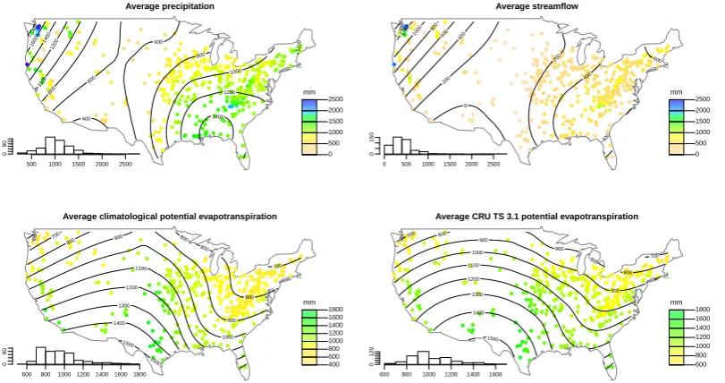
The basins in the US MOPEX dataset cover a variety of hydro-climatic conditions, which can be seen in the map-ping of long-term average variables (P , Q, Ep,clim, Ep,CRU) in Fig. 1. The basins with most precipitation are found in the Northwest, the Southeast and along the east coast. The central part of the US receives considerably less precipita-tion, which is a continental climate effect intensified by the mountain ranges in the west and east, blocking west to east atmospheric moisture transport. Potential evapotranspiration obeys a north to south increasing gradient, which is modu-lated by the continental climate in the central US. The bot-tom maps show the climatological Ep estimates from the evaporation atlas (Farnsworth and Thompson, 1982) and the long-term averages of the CRU TS 3.1 potential evapotran-spiration estimates Ep,CRU. The long-term basin averages ofEp,CRUshow the highest spatial correlation (r=0.89) to Ep,clim, while Hamon (r=0.57) and Hargreaves (r=0.46) have lower correlation and somewhat different spatial pat-terns. Therefore, we selectedEp, CRUfor further analysis.
● ● ● ● ● ● ● ● ● ●●●● ● ● ●● ● ● ● ● ● ● ● ● ● ● ● ●●● ●●●● ● ●● ●●●● ●●●●● ●●● ●● ●● ●●●● ● ●● ●● ● ● ● ● ● ● ●●●● ● ● ● ● ●● ● ● ● ● ● ● ●● ● ● ● ● ● ● ● ●● ● ● ● ● ● ● ●● ● ● ● ●● ● ● ●●●●●●● ● ● ● ● ● ● ●●●●●●●● ● ● ● ●● ● ● ● ● ● ● ● ● ● ● ●● ● ● ● ● ● ● ● ● ● ● ● ●● ● ● ● ● ● ● ● ● ● ● ● ●●● ●● ●●● ●● ● ● ●● ● ● ● ● ● ● ● ● ● ● ●●●● ● ● ●●●●●● ●●● ●● ● ● ●●●● ●●●●●● ●●●● ● ● ● ●● ● ●● ● ● ● ●● ● ● ● ● ● ● ● ● ● ● ● ● ● ● ●● ●● ● ● ● ●● ● ● ● ● ● ● ● ● ●●● ● ● ● ● ●●●●●● ● ● ●● ● ● ●● ●●●● ●●● ● ● ● ●●● ● ●●●●● ● ● ● ● ● ● ●● ● ● ●●● ● ● ● ● ● ●● ● ●● ● ● ● ● ● ● ●●● ● ● ●● ● ● ● ● ● ● ● ● ● ●● ●●●● ● ● ● ● ● ●● ● ● ● ● ● ● ●● ●● ● ● ● ● ● ● ● ● ● ●● ● ●● ● ● ● ● ● ●●●●● ● ● ● ● ●● ●● ● ●● ● ● ●● ● ● ● ● ● ● ● ● ● ● Average precipitation 400 600 600 800 800 1000 1000 1200 1200 1200 1400 1400 1600
Frequency 0 500 1000 1500 2000 2500
80 0 500 1000 1500 2000 2500 mm ● ● ● ● ● ● ● ● ● ●●●● ● ● ●● ●● ● ● ● ● ● ● ● ● ● ●●● ●●●● ● ● ● ●●●● ● ●●●● ●●● ●● ● ● ●●●● ● ●● ●● ● ● ● ● ● ● ●●●● ● ● ● ● ●●● ● ● ● ● ● ●● ● ● ● ● ● ● ● ●● ● ● ● ● ● ● ●● ● ● ● ●● ● ● ●●●●●●● ● ● ● ● ● ● ●●●●●●●● ● ● ● ●● ● ● ● ● ● ● ● ● ● ●●● ● ● ● ● ● ● ● ● ● ● ● ● ● ● ● ● ● ● ●●● ● ● ● ● ● ● ●● ●●● ●● ● ● ●● ● ● ● ● ● ● ●● ● ● ●●●● ● ●●●●●●● ●●● ●● ● ● ●● ● ● ● ●●●●● ●●●● ● ● ● ●● ● ●● ● ● ● ●● ● ●● ● ● ● ● ● ● ● ● ● ● ●● ●● ● ● ● ●● ● ● ● ● ● ● ● ● ●●● ● ● ● ● ●●●●●● ● ● ●● ● ● ●● ●●●● ● ● ● ● ● ● ●●● ● ●●●●● ●● ●● ● ● ●● ● ● ●●● ● ● ●● ● ●● ●●● ● ● ● ● ● ● ●●● ● ● ● ● ● ● ● ● ● ● ● ● ● ●● ●●●● ● ● ● ● ● ●● ● ● ● ● ● ● ●● ●● ● ● ● ● ● ● ● ● ● ●● ● ●● ● ● ● ● ● ●●●●● ● ● ● ● ●● ●● ● ●● ● ● ● ● ● ● ● ● ● ● ● ● ● ● Average streamflow 0 200 200 400 400 400 600 600 800 1000 1200
Frequency 0 0 500 1000 1500 2000 2500
150 0 500 1000 1500 2000 2500 mm ● ● ● ● ● ● ● ● ●●●● ● ● ●● ● ● ● ● ● ● ● ● ● ● ● ●● ● ●●●●●●● ●●●● ●●●●● ●●● ●● ●● ●● ●● ● ●● ●● ● ● ● ● ● ● ●●●● ● ● ● ● ●● ● ● ● ● ● ● ●●● ● ● ● ● ● ● ●● ● ● ● ● ● ● ●● ● ● ● ● ● ● ● ●●●●●●● ● ● ● ● ● ● ●●●●●●●● ● ● ● ●● ● ● ● ● ● ● ● ● ● ● ●● ● ● ● ● ● ● ● ● ● ● ● ●● ● ●●● ● ● ● ● ● ● ● ●●● ●● ●●● ●● ● ● ●● ● ● ● ● ● ● ● ● ● ● ●●● ● ● ●●●●●● ●●● ●● ● ● ●●●● ●● ● ●● ● ●●●● ●● ● ●● ● ●● ● ● ● ●● ● ● ● ● ● ● ● ● ● ●● ● ● ● ●● ●● ● ● ● ●● ● ● ● ● ● ● ● ● ●●● ● ● ● ● ●●●●● ● ● ● ●● ● ● ●● ●●●● ●●● ● ● ● ●●● ● ●●●●● ● ● ● ● ● ● ●● ● ● ● ● ● ● ● ● ● ● ●● ● ●● ● ● ● ● ● ● ●●● ● ● ●● ● ● ● ● ● ● ● ● ● ●● ●●●● ● ● ● ● ● ●● ● ● ● ● ● ● ●● ●● ● ● ● ● ● ● ● ● ●● ● ●● ● ● ● ● ● ●●●●● ● ● ● ● ●● ●● ● ●● ● ● ●● ● ● ● ● ● ● ● ● ● ●
Average climatological potential evapotranspiration
700 700 800 800 800 800 900 900 1000 1100 1200 1300 1400 1500 1500
Frequency 0 600 800 10001200140016001800
80 400 600 800 1000 1200 1400 1600 1800 mm ● ● ● ● ● ● ● ● ● ●●●● ● ● ●● ●● ● ● ● ● ● ● ● ● ● ●● ● ●●●●●●● ●●●● ● ●●●● ●●● ●● ● ● ●● ●● ● ●● ●● ● ● ● ● ● ● ●●●● ● ● ● ● ●●● ● ● ● ● ● ●●● ● ● ● ● ● ● ●● ● ● ● ● ● ● ●● ● ● ● ● ● ● ● ●●●●●●● ● ● ● ● ● ● ●●●●●●●● ● ● ● ●● ● ● ● ● ● ● ● ● ● ●●● ● ● ● ● ● ● ● ● ● ● ● ● ● ● ●●● ● ●●● ● ● ● ● ● ● ●● ●●● ●● ● ● ●● ● ● ● ● ● ● ●● ● ● ●●●● ● ●●●●●●● ●●● ●● ● ● ●●●● ● ● ● ●● ● ●●●● ●● ● ●● ● ●● ● ● ● ●● ● ●● ● ● ● ● ● ● ● ● ● ● ● ●● ●● ● ● ● ●● ● ● ● ● ● ● ● ● ●●● ● ● ● ● ●●●●● ● ● ● ●● ● ● ●● ●●●● ● ●● ● ● ● ●●● ● ●●●●● ●● ●● ● ● ●● ● ● ● ● ● ● ● ●● ● ●● ●●● ● ● ● ● ● ● ●●● ● ● ● ● ● ● ● ● ● ● ● ● ● ●● ●●●● ● ● ● ● ● ●● ● ● ● ● ● ● ●● ●● ● ● ● ● ● ● ● ● ● ●● ● ●● ● ● ● ● ● ●●●●● ● ● ● ● ●● ●● ● ●● ● ● ● ● ● ● ● ● ● ● ● ● ● ●
Average CRU TS 3.1 potential evapotranspiration
700 700 800 800 800 800 900 900 1000 1100 1200 1300 1400 1500
Frequency 600 800 1000 1200 1400 1600
[image:6.595.98.504.62.276.2]0 120 600 800 1000 1200 1400 1600 1800 mm
Fig. 1. Long-term annual average of hydroclimatic variables of the US MOPEX dataset (1949–2003). The contour lines are derived from
fitted polynomial surfaces using the R function stats::loess (R Development Core Team, 2011) of the variables using the river gauge locations. The map of the US is taken from the maps package (Becker et al., 2011).
●●● ●● ● ● ● ● ● ● ● ● ● ● ●● ● ● ●● ● ● ● ● ● ● ● ● ● ● ● ● ● ● ● ● ●● ● ● ● ● ●●● ● ● ● ● ●● ●● ●● ● ● ●● ● ● ● ● ● ● ● ● ● ● ● ● ● ● ● ● ● ●●● ● ● ● ● ● ● ● ● ● ● ●● ● ● ● ● ● ● ● ● ● ● ● ● ● ●●● ● ● ● ● ● ● ● ●● ● ● ● ● ● ● ● ● ●● ● ● ● ●● ●●●● ● ● ● ● ● ● ● ● ● ● ● ● ● ● ● ● ● ● ● ● ● ● ● ● ● ● ● ● ●● ●●●● ● ● ● ● ● ● ● ● ● ● ● ● ● ● ● ● ●● ● ●● ● ● ● ● ● ● ● ● ● ● ● ● ●●● ● ● ● ● ● ● ● ● ● ● ● ● ●●●● ● ●●●●●●● ● ● ●● ● ● ● ●●● ● ● ● ● ● ● ● ● ● ●● ●● ● ● ● ● ●●● ● ●● ● ● ● ● ● ● ● ● ● ● ● ● ●● ● ● ● ● ● ● ● ● ● ● ● ● ● ● ● ● ● ● ● ● ● ● ● ● ● ● ● ● ● ● ● ●● ● ● ● ● ● ● ●● ● ● ● ● ● ● ● ● ● ● ● ● ● ● ● ● ● ● ● ● ● ● ● ● ● ● ● ● ● ● ●●● ● ● ● ● ● ● ● ● ● ● ● ● ● ● ● ● ● ● ● ● ● ● ● ● ● ● ● ● ● ● ● ● ● ● ● ●● ● ● ● ● ● ● ● ● ● ● ● ● ● ● ●● ● ● ● ● ● ● ● ● ● ● ● ● ● ● ● ● ● ● ● ● ● ● ● ● ● ●
0 1 2 3 4 5
0.0 0.2 0.4 0.6 0.8 1.0
EpP
ET P water limit energy limit ●●● ●● ● ● ● ● ● ● ● ● ● ● ●● ● ● ●● ● ● ● ● ● ● ● ● ● ● ● ● ● ● ● ● ●● ● ● ● ● ●●● ● ● ● ● ●● ●● ●● ● ● ●● ● ● ● ● ● ● ● ● ● ● ● ● ● ● ● ● ● ●●● ● ● ● ● ● ● ● ● ● ● ●● ● ● ● ● ● ● ● ● ● ● ● ● ● ●●● ● ● ● ● ● ● ● ●● ● ● ● ● ● ● ● ● ●● ● ● ● ●● ●●●● ● ● ● ● ● ● ● ● ● ● ● ● ● ● ● ● ● ● ● ● ● ● ● ● ● ● ● ● ●● ●●●● ● ● ● ● ● ● ● ● ● ● ● ● ● ● ● ● ●● ● ●● ● ● ● ● ● ● ● ● ● ● ● ● ●●● ● ● ● ● ● ● ● ● ● ● ● ● ●●●● ● ●●●●●●● ● ● ●● ● ● ● ●●● ● ● ● ● ● ● ● ● ● ●● ●● ● ● ● ● ●●● ● ●● ● ● ● ● ● ● ● ● ● ● ● ● ●● ● ● ● ● ● ● ● ● ● ● ● ● ● ● ● ● ● ● ● ● ● ● ● ● ● ● ● ● ● ● ● ●● ● ● ● ● ● ● ●● ● ● ● ● ● ● ● ● ● ● ● ● ● ● ● ● ● ● ● ● ● ● ● ● ● ● ● ● ● ● ●●● ● ● ● ● ● ● ● ● ● ● ● ● ● ● ● ● ● ● ● ● ● ● ● ● ● ● ● ● ● ● ● ● ● ● ● ●● ● ● ● ● ● ● ● ● ● ● ● ● ● ● ●● ● ● ● ● ● ● ● ● ● ● ● ● ● ● ● ● ● ● ● ● ● ● ● ● ● ● Budyko function ● ● ● ● ● ● ● ● ● ● ● ● ● ● ● ● ● ● ● ● ● ● ● ● ● ● ● ● ●● ● ● ●● ● ● ● ● ● ● ● ● ● ● ●● ● ● ● ● ● ● ● ● ● ● ● ● ● ● ● ● ● ●●●●●● ● ●● ● ● ● ● ● ● ● ● ● ● ●● ● ● ●● ● ● ● ● ● ● ● ● ●● ●● ● ● ●● ● ● ●● ● ● ● ● ● ● ● ● ● ● ● ●●●● ● ● ● ● ● ● ●●● ● ● ●● ● ● ● ● ● ● ●● ● ● ●●● ● ● ● ● ● ● ● ● ● ● ● ●● ● ● ● ● ● ●●● ● ● ● ● ● ● ● ● ● ● ● ● ● ● ● ●●● ● ● ● ● ● ● ● ● ● ● ● ● ● ● ● ●●●● ● ● ● ●● ● ● ●● ● ● ● ●●● ●●●● ● ● ●●● ● ● ● ● ●●●●●● ●●● ● ● ●● ● ● ● ● ● ● ● ● ● ● ● ●●●● ● ● ● ● ● ● ● ● ● ● ● ●● ● ● ● ● ● ● ● ● ●● ● ● ● ● ● ●● ● ● ● ● ● ● ●●● ●● ● ● ● ● ● ●● ● ● ● ● ● ● ● ● ● ● ● ● ● ●● ● ●●● ● ● ● ● ● ● ● ● ● ● ● ● ●● ● ● ● ● ● ●● ● ● ● ● ● ● ●●● ● ● ●● ● ● ● ● ● ● ● ● ● ● ● ● ● ● ● ● ● ● ● ● ● ● ● ● ● ● ● ● ● ● ● ● ● ● ● ● ● ● ● ● ● ● ● ● ● ● ● ● ● ● ● ● ● ● ● ● ● ● ●● ● ● ● ● ●
0.0 0.2 0.4 0.6 0.8 1.0
0.0 0.2 0.4 0.6 0.8 1.0
W = Q/P
U = 1 −
ET Ep w ater limit energy limit ● ● ● ● ● ● ● ● ● ● ● ● ● ● ● ● ● ● ● ● ● ● ● ● ● ● ● ● ●● ● ● ●● ● ● ● ● ● ● ● ● ● ● ●● ● ● ● ● ● ● ● ● ● ● ● ● ● ● ● ● ● ●●●●●● ● ●● ● ● ● ● ● ● ● ● ● ● ●● ● ● ●● ● ● ● ● ● ● ● ● ●● ●● ● ● ●● ● ● ●● ● ● ● ● ● ● ● ● ● ● ● ●●●● ● ● ● ● ● ● ●●● ● ● ●● ● ● ● ● ● ● ●● ● ● ●●● ● ● ● ● ● ● ● ● ● ● ● ●● ● ● ● ● ● ●●● ● ● ● ● ● ● ● ● ● ● ● ● ● ● ● ●●● ● ● ● ● ● ● ● ● ● ● ● ● ● ● ● ●●●● ● ● ● ●● ● ● ●● ● ● ● ●●● ●●●● ● ● ●●● ● ● ● ● ●●●●●● ●●● ● ● ●● ● ● ● ● ● ● ● ● ● ● ● ●●●● ● ● ● ● ● ● ● ● ● ● ● ●● ● ● ● ● ● ● ● ● ●● ● ● ● ● ● ●● ● ● ● ● ● ● ●●● ●● ● ● ● ● ● ●● ● ● ● ● ● ● ● ● ● ● ● ● ● ●● ● ●●● ● ● ● ● ● ● ● ● ● ● ● ● ●● ● ● ● ● ● ●● ● ● ● ● ● ● ●●● ● ● ●● ● ● ● ● ● ● ● ● ● ● ● ● ● ● ● ● ● ● ● ● ● ● ● ● ● ● ● ● ● ● ● ● ● ● ● ● ● ● ● ● ● ● ● ● ● ● ● ● ● ● ● ● ● ● ● ● ● ● ●● ● ● ● ● ● 0 1 2 3 4 5
EpP
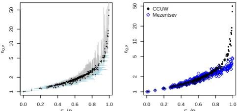
Fig. 2. Budyko (left) and U W space (right) plots of the period
(1949–2003) of the MOPEX dataset.Epis obtained from the CRU
TS 3.1Epproduct. The 1:1 line in theU Wspace diagram
sepa-rates areas with energy limitation (Ep/P <1) and water limitation
(Ep/P >1). Grey lines indicate the water and energy limits.
Budyko’s function explains 69 % of the variance. The aridity indexEp/P of the basins ranges between 0.25 and 5.52, with most basins clustering around 1. The right panel of Fig. 2 displays the relationship of the non-dimensional measures W andU, referred to as UW space. Note thatW=1−ET
P ,
wherebyET/P is used in the Budyko plot on the ordinate. A thorough discussion of the relationship between both spaces can be found in Renner et al. (2012). The hydro-climatic data cover the UW space, meaning that there is a large va-riety of hydro-climate conditions in the dataset.Wis ranging between 0 and 1, whileU also has one negative value (not shown because of the scales used for the axes). This is prob-ably due to an underestimation ofEp, CRUfor this basin.
4.2 Climate sensitivity of streamflow
Next, we compare the climate sensitivity coefficients of the CCUW with the Budyko framework using the long-term av-erages of the MOPEX dataset. In particular, we concentrate on the sensitivity of streamflow to precipitationεQ,P.
Using the CCUW approach,εQ,P;CCUWis determined by Eq. (4), which shows that the coefficient is dependent on the aridity index and the inverse of the runoff ratio. In particu-lar, the correlation of the sensitivity coefficient to the aridity index (correlationr=0.53) is much lower than the correla-tion toP /Q(r=0.99). This means that, using the CCUW hypothesis, the inverse of the runoff ratio (P /Q) is the main controlling factor in determining runoff sensitivity to climate. To further illustrate this functional relationship, we plot εQ,Pin Fig. 3 as a function of the evaporation ratio, which is
directly related to the inverse of the runoff ratio, but bounded between 0 and 1. From the left panel (black dots), we see that the estimate of the CCUW method (εQ,P;CCUW) is primarily
and nonlinearly determined byET/P. To estimate the uncer-tainty in estimation ofεQ,P;CCUW, we computedεQ,P;CCUW for each year in the 55-yr period and display the interquar-tile range (25 %–75 % perceninterquar-tile range) of all those annual sensitivity coefficients as vertical grey lines. The uncertainty ranges increase withET/P. For values of ET/P >0.6, the ranges get more apparent with about 25 % of εQ,P, which
[image:6.595.48.290.340.456.2]0.0 0.2 0.4 0.6 0.8 1.0 1 2 5 10 20 50
ETP
εQ,P ● ● ● ●● ● ● ● ● ● ● ● ● ● ● ● ●● ● ● ● ● ● ● ● ●● ● ● ● ● ●●●●● ● ● ●●●● ● ●● ● ● ● ● ● ● ●● ●●●●● ● ● ● ● ● ● ● ● ●● ● ● ● ● ● ● ● ● ● ● ● ● ● ● ● ● ● ● ● ● ● ● ● ●●● ● ● ● ●●● ● ● ● ● ● ● ● ●● ● ● ● ●●●●● ● ●● ● ● ●● ●● ● ● ●● ● ● ● ● ●● ● ●● ● ● ●● ● ●●●●●● ● ● ● ● ● ●● ● ●● ● ● ● ● ● ●●● ● ● ● ●● ● ●● ● ●● ● ● ● ● ●●●●●● ●● ● ●● ● ●●● ● ● ● ● ● ● ●● ● ●● ●●● ● ● ● ● ● ● ●●●● ● ●●●●●●● ● ● ●●● ● ● ● ● ● ● ● ●● ● ● ● ●● ●●●● ● ● ● ●●●● ●●● ● ● ● ● ● ● ● ● ● ● ● ● ●● ● ● ● ● ● ● ● ● ● ● ● ● ● ● ● ● ● ● ● ● ● ●● ● ●● ●● ● ● ● ● ● ● ● ● ● ● ● ●● ● ● ● ● ● ● ●● ● ● ● ● ● ● ● ● ● ● ● ● ● ● ● ●● ● ● ● ● ●●●● ● ● ● ● ● ● ● ● ● ● ●● ● ● ● ● ● ● ●● ● ● ● ● ● ● ● ● ● ● ● ● ● ● ● ● ● ● ● ● ● ● ● ● ● ● ● ● ● ●● ● ● ● ● ● ●● ● ● ● ● ● ● ●● ●●●● ● ● ● ● ● ● ●● ●
0.0 0.2 0.4 0.6 0.8 1.0
1 2 5 10 20 50
ETP
[image:7.595.46.288.61.174.2]εQ,P ● ● ● ●● ● ● ● ● ● ● ● ● ● ● ● ●● ● ● ● ● ● ● ● ●● ● ● ● ● ●●●●● ● ● ●●●● ● ●● ● ● ● ● ● ● ●● ●●●●● ● ● ● ● ● ● ● ● ●● ● ● ● ● ● ● ● ● ● ● ● ● ● ● ● ● ● ● ● ● ● ● ● ●●● ● ● ● ●●● ● ● ● ● ● ● ● ●● ● ● ● ●●●●● ● ●● ● ● ●● ●● ● ● ●● ● ● ● ● ●● ● ●● ● ● ●● ● ●●●●●● ● ● ● ● ● ●● ● ●● ● ● ● ● ● ●●● ● ● ● ●● ● ●● ● ●● ● ● ● ● ●●●●●● ●● ● ●● ● ●●● ● ● ● ● ● ● ●● ● ●● ●●● ● ● ● ● ● ● ●●●● ● ●●●●●●● ● ● ●●● ● ● ● ● ● ● ● ●● ● ● ● ●● ●●●● ● ● ● ●●●● ●●● ● ● ● ● ● ● ● ● ● ● ● ● ●● ● ● ● ● ● ● ● ● ● ● ● ● ● ● ● ● ● ● ● ● ● ●● ● ●● ●● ● ● ● ● ● ● ● ● ● ● ● ●● ● ● ● ● ● ● ●● ● ● ● ● ● ● ● ● ● ● ● ● ● ● ● ●● ● ● ● ● ●●●● ● ● ● ● ● ● ● ● ● ● ●● ● ● ● ● ● ● ●● ● ● ● ● ● ● ● ● ● ● ● ● ● ● ● ● ● ● ● ● ● ● ● ● ● ● ● ● ● ●● ● ● ● ● ● ●● ● ● ● ● ● ● ●● ●●●● ● ● ● ● ● ● ●● ● ●CCUW Mezentsev
Fig. 3. Sensitivity coefficients of streamflow to precipitation as
function of ET/P. Left panel: εQ,P;CCUW computed for the
CCUW method. Dots representεQ,P;CCUW using long-term
av-erage data of the respective basin. Vertical grey lines depict the interquartile range ofεQ,P;CCUW estimated for each year in the
record, while light blue horizontal lines show the interquartile range forET/P. Right panel:εQ,P for different methods using long-term
averages of (P , Ep, Q) of the period 1949–2003. Note that a
loga-rithmic y-axis is used for both plots.
of individual years or periods can have large impacts on the resulting streamflow.
The right panel of Fig. 3 provides a comparison of the sensitivity estimates of CCUW with the parametric Budyko function approach of Roderick and Farquhar (2011) using the Mezentsev function, withnestimated for each basin sep-arately. The non-parametric Budyko sensitivity approaches are determined by aridity only (Arora, 2002) and have large differences to CCUW, already at medium values of ET/P (not shown). The parametric Budyko function ap-proach yields similar sensitivities as the CCUW apap-proach forET/P <0.9. This is due to the parametern, which inher-ently includes some dependency toET/P (the correlation of εQ,P;MeztoP /Qisr=0.63). However, it can be shown that there is an upper limit for the sensitivity coefficient, which is set byn+1. Here, we estimated the largest value of n for the given dataset withn=4 and the largest sensitivity
withεQ,P ,Mez=4.7. In contrast, the sensitivity of
stream-flow to precipitation estimated by the CCUW approach is not bounded and proportional to the inverse of the runoff ratio. However, the theoretical assessment of the CCUW hypothe-sis by Renner et al. (2012) revealed that these large stream-flow sensitivity estimates for strongly water-limited basins are probably incorrect, because the CCUW does not obey Budyko’s water limit.
4.3 Assessment of observed and predicted changes in
streamflow
Next, we evaluate the introduced analytical streamflow change prediction methods under past hydro-climatic changes in the contiguous US using data covering the wa-ter years from 1949 to 2003. As the approaches assume steady-state conditions, we evaluate the changes by subdi-viding the data into two periods, 1949–1970 and 1971–2003.
Table 1. Statistics of the average change of the threeEpestimates.
The first three columns depict quantiles of1Ep; the forth and fifth
columns denote the relative frequency of basins with significant change (α=0.05, two sample t-test) forEpand the aridity index
(AR).
10 % 50 % 90 % 1Ep≤α 1AR≤α
[mm] [mm] [mm] [%] [%] CRU −32 −8 13 13 19 Hargreaves −41 −23 −6 69 40 Hamon −16 −6 9 6 26
This choice is in accordance with the recent study of Wang and Hejazi (2011). They justify their selection with a proba-ble step increase in precipitation and in streamflow in large parts of the US around the year 1970 (McCabe and Wolock, 2002).
4.3.1 Hydro-climatic changes in the US
[image:7.595.312.546.126.192.2]Change in precipitation, ∆P
t−test significant not significant
20 40
40 60
60 60 80
80
100
100
120
120
140
−235 −118 −47 47 118 235
∆P [mm]
Frequency
−100 0 50 100 150 200 250
0
100
t−test significant not significant Change in potential evaporation, ∆Ep,CRU
−30
−25 −20
−20 −15 −10 −5
−5 −5 0
0 0
5
5
5 5
5 10
10 10 15
15
20 20
25
−62 −31 −12 12 31 62
∆Ep,CRU [mm]
Frequency
−60 −40 −20 0 20 40
0
40
80
t−test significant not significant Change in streamflow, ∆Q
−80 −60
−60 −40
−20
0
0
20
20 40
40 60
60 60
60
80
−171 −86 −34 34 86 171
∆Q [mm]
Frequency
−200 −100 0 100 200
0
50
150
∆α = 0.05 − P Ep P,Ep Q Q,P Q,P,Ep Classification of significant (α= 0.05) hydro−climatic changes
− P Ep P,Ep Q Q,P Q,P,Ep
0
50
150
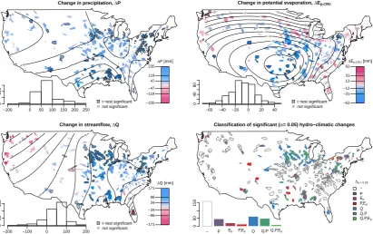
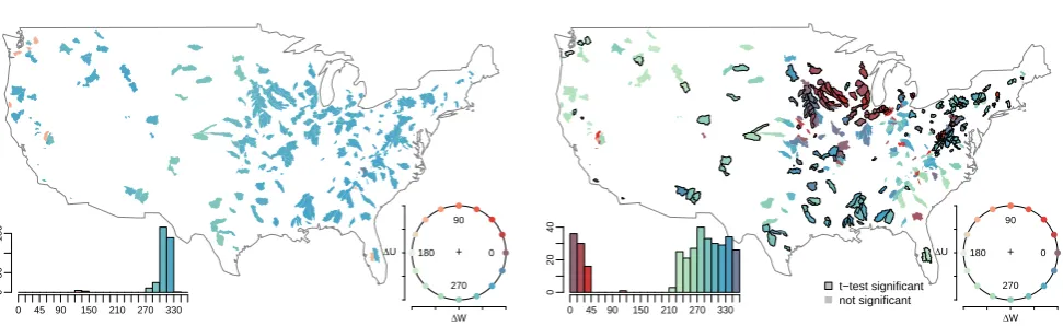
Fig. 4. Maps of absolute change in hydro-climatic variables of the MOPEX dataset, comparing changes between the periods 1949–1970 and
[image:8.595.93.505.63.321.2]1971–2003. Annual changes are given in millimeter. Significant changes in the mean of both periods are tested by univariate two-sample t-tests withα=0.05 and are denoted by a grey borderline. For each variable, a histogram of the changes is given in the lower left corner. The map in panel (d) provides a classification based on the univariate t-tests.
Table 2. Pearson correlation coefficients for the average change between the two periods, assessed for all basins with data available.
Sig-nificance of correlation is denoted with letters (a 0.001,b0.01,c0.05), with significant correlations (α <0.05) set in bold for visual aid.
1Q 1P 1EP ,CRU 1EP ,HAR 1EP ,HAM 1T 1Q
1P 0.57a
1EP, CRU −0.18a −0.17b
1EP, HAR −0.13c −0.01 0.08
1EP, HAM −0.23a −0.23a 0.30a −0.04
1T −0.22a −0.19a 0.24a 0.01 0.96a
1TR −0.18a −0.01 0.13b 0.99a −0.02 0.02
temperature and diurnal temperature range (Table 2). This finding further supports the usage of the CRU Ep dataset. The top right map of Fig. 4 shows that negative significant changes in averageEpare common in the southern central parts (about−30 mm) and a few patches throughout the US. Both the increase in precipitation and the decrease in po-tential evapotranspiration should ideally lead to an increase in annual streamflow. This is supported by the strong positive correlation with precipitation changes and the negative corre-lation coefficients with theEpchanges (Table 2). Further, we find that 32 % of the basins show a significant increase. The map in the bottom left panel of Fig. 4 shows that basins with significant increases in streamflow are predominantly found
● ● ● ● ● ●● ● ● ● ● ● ● ●● ● ● ● ● ●●● ● ● ● ●● ● ● ● ●● ● ● ● ● ● ●● ● ● ● ● ● ●● ● ● ● ● ●● ● ● ● ● ● ● ● ● ● ● ● ● ● ● ● ●● ● ● ● ● ● ● ● ● ● ●●● ● ● ● ● ● ● ● ●● ● ● ● ● ● ● ● ● ●●●●● ● ● ● ●● ● ● ● ● ● ● ● ●● ● ● ● ●● ● ● ● ● ● ● ● ● ●●● ● ● ● ● ● ● ● ● ● ● ●● ● ● ●●● ● ● ● ● ● ● ● ● ● ● ● ● ● ● ● ● ● ● ● ● ● ● ● ● ● ● ● ● ● ● ● ● ● ● ● ● ● ●●●●●● ●●●●● ● ●● ● ● ● ● ● ●● ●● ● ● ● ● ●●● ●● ● ●● ●● ● ● ● ● ● ● ● ● ● ● ● ● ●● ● ● ● ● ●●●● ● ●●● ● ● ● ●● ● ● ● ● ● ● ● ● ● ● ● ● ●●● ●● ● ● ● ● ● ●● ● ● ● ● ● ● ● ● ● ● ● ● ● ● ● ● ● ● ● ● ● ● ● ● ● ● ● ● ● ●● ● ● ● ● ●● ● ●● ● ● ● ● ● ● ● ●●●● ● ● ● ● ● ● ● ● ● ● ● ● ● ● ● ● ● ● ● ● ●
−150 −50 0 50 100 150
−50
0
50
100
150
∆Qobs [mm]
∆
Qpred
[mm] ● ●
● ● ● ●● ● ● ● ● ● ● ●● ● ● ● ● ●●● ● ● ● ●● ● ● ● ●● ● ● ● ● ● ●● ● ● ● ● ● ●● ● ● ● ● ●● ● ● ● ● ● ● ● ● ● ● ● ● ● ● ● ●● ● ● ● ● ● ● ● ● ● ●●● ● ● ● ● ● ● ● ●● ● ● ● ● ● ● ● ● ●●●●● ● ● ● ●● ● ● ● ● ● ● ● ●● ● ● ● ●● ● ● ● ● ● ● ● ● ●●● ● ● ● ● ● ● ● ● ● ● ●● ● ● ●●● ● ● ● ● ● ● ● ● ● ● ● ● ● ● ● ● ● ● ● ● ● ● ● ● ● ● ● ● ● ● ● ● ● ● ● ● ● ●●●●●● ●●●●● ● ●● ● ● ● ● ● ●● ●● ● ● ● ● ●●● ●● ● ●● ●● ● ● ● ● ● ● ● ● ● ● ● ● ●● ● ● ● ● ●●●● ● ●●● ● ● ● ●● ● ● ● ● ● ● ● ● ● ● ● ● ●●● ●● ● ● ● ● ● ●● ● ● ● ● ● ● ● ● ● ● ● ● ● ● ● ● ● ● ● ● ● ● ● ● ● ● ● ● ● ●● ● ● ● ● ●● ● ●● ● ● ● ● ● ● ● ●●●● ● ● ● ● ● ● ● ● ● ● ● ● ● ● ● ● ● ● ● ● ● ●CCUW Mezentsev ● ● ● ● ● ●● ● ● ● ● ● ● ●●● ● ● ● ●● ●●● ● ●● ● ● ● ●● ● ●● ● ●●● ● ● ●● ● ● ● ●● ● ● ● ● ● ● ● ● ● ● ●● ● ● ● ● ● ● ● ● ● ●● ● ● ● ●● ● ● ●●● ● ● ● ● ● ●●● ●● ● ●● ● ● ●● ● ●●●●● ● ●●●● ●● ● ● ● ● ● ● ● ●● ● ● ● ●● ● ● ●● ●●●● ● ● ● ● ● ●●● ●● ● ● ●● ● ● ●● ● ● ● ● ● ●● ● ● ● ● ● ● ● ● ● ● ●● ● ● ● ● ● ● ● ● ● ● ● ● ● ● ●● ●●●●●●●●●●● ●● ● ● ● ● ● ● ●● ●●● ● ● ●●● ●●● ● ●●●● ● ● ●●●●● ● ●● ● ● ● ● ● ● ● ● ● ●●●● ●● ● ●● ● ●● ●● ● ● ● ● ● ●● ● ● ● ● ● ● ● ● ● ● ● ● ● ●● ● ● ● ● ● ● ●● ● ● ● ● ●● ● ● ● ● ● ● ● ● ● ●●● ● ● ● ●● ● ●● ● ● ● ● ●● ● ● ● ● ● ● ●● ● ●● ● ● ● ● ● ● ● ● ● ● ●● ● ● ● ● ● ●● ●●
−50 0 50 100 150
−50
0
50
100
150
∆QCCUW [mm]
[image:9.595.47.288.62.176.2]∆ QM e z [mm] ● ● ● ● ● ●● ● ● ● ● ● ● ●●● ● ● ● ●● ●●● ● ●● ● ● ● ●● ● ●● ● ●●● ● ● ●● ● ● ● ●● ● ● ● ● ● ● ● ● ● ● ●● ● ● ● ● ● ● ● ● ● ●● ● ● ● ●● ● ● ●●● ● ● ● ● ● ●●● ●● ● ●● ● ● ●● ● ●●●●● ● ●●●● ●● ● ● ● ● ● ● ● ●● ● ● ● ●● ● ● ●● ●●●● ● ● ● ● ● ●●● ●● ● ● ●● ● ● ●● ● ● ● ● ● ●● ● ● ● ● ● ● ● ● ● ● ●● ● ● ● ● ● ● ● ● ● ● ● ● ● ● ●● ●●●●●●●●●●● ●● ● ● ● ● ● ● ●● ●●● ● ● ●●● ●●● ● ●●●● ● ● ●●●●● ● ●● ● ● ● ● ● ● ● ● ● ●●●● ●● ● ●●●● ● ●● ● ● ● ● ● ●● ● ● ● ● ●● ● ● ● ● ● ● ● ●● ● ● ● ● ● ● ●● ● ● ● ● ●● ● ● ● ● ● ● ● ● ● ●●● ● ● ● ●● ● ●● ● ● ● ● ●● ● ● ● ● ● ● ●● ● ●● ● ● ● ● ● ● ● ● ● ● ●● ● ● ● ● ● ●● ●● 0.0 0.2 0.4 0.6 0.8 1.0 ET/P
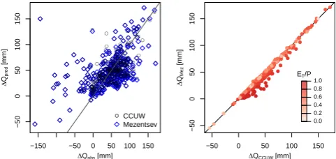
Fig. 5. Left: Scatterplot of observed vs. predicted annual average
changes in streamflow for MOPEX dataset without stations with missing data. The vertical difference to the 1:1 line depicts the deviation of the prediction to the observed value. Right: predicted change in streamflow due to climatic changes, comparing the es-timates of the Budyko framework with the CCUW eses-timates. The colour of the dots represents the evaporation ratioET/P.
4.3.2 Evaluation of streamflow change predictions
In the previous subsection, we described the changes ob-served in precipitation, potential evapotranspiration and streamflow by comparing the long-term averages of two pe-riods. Now we aim to predict the change in streamflow, using the climate sensitivity approaches of the CCUW method (i.e. application of Eq. 5) and the Budyko approach illustrated by Roderick and Farquhar (2011). For the Budyko approach, we use Eq. (8) and the functional form of Mezentsev (1955). In particular, we use the hydro-climatic state of the first period, described byP0, Ep,0, Q0, as well as the climatic states of the second periodP1, Ep,1to predict the streamflow of the second periodQ1. Then, we evaluate the accuracy of stream-flow prediction by using the observed1Qobsand predicted change1Qclimsignals.
A scatterplot of predicted versus observed changes is shown in the left panel of Fig. 5, where dots close to the 1:1 line indicate good predictions. While most dots scatter around the 1:1 line, there is a considerable num-ber of basins where prediction and observation are com-pletely different. There is also no indication if one method is more realistic than the other. Based on all basins (N=
351), both methods yield similar differences compared with the observed change in streamflow (RMSECCUW=40.9 mm, RMSEMez=41.3 mm). A direct comparison is shown as scatterplot in the right panel of Fig. 5. The graph indicates that there is a general agreement between both estimates (r=0.99). The largest differences between both methods are found for basins with very high evaporation ratios. In this case, CCUW predicts larger changes than the Budyko ap-proach, which was already discussed above. These changes are small in absolute values, but quite large when seen rela-tive to the annual totals of streamflow.
4.3.3 Separating the influence of climate and land-use
impacts on streamflow
From the maps in Fig. 4, it is apparent that basins with sig-nificant changes in streamflow do not necessarily match with those having significant changes in the climatic variables (P , Ep). Such inconsistency between climatic and stream-flow trends was also reported in previous literature such as in Lettenmaier et al. (1994).
For further analysis, we combined the results of the univariate t-tests (α=0.05), which resulted in 9 different classes. These are further aggregated to the four different hypotheses on streamflow change elaborated in Sect. 2.4. In Table 3, we provide summary statistics for each class. The map in Fig. 4d shows the location of the groups in the US, with a bar plot in the lower left corner showing the counts of each group. For most basins (46 %), we found no sig-nificant change in any of the three observed variables. The group of basins where only streamflow changed significantly while climatic variables show insignificant changes is large and consists of 17 % of all basins. These are mostly found in the central north of the US, west of the Great Lakes. In the other extreme, there are basins, where significant cli-matic changes occurred, while streamflow did not change significantly. Combining these classes to the “climate only” group, 21 % of the basins are affected. For this group, red-dish colours have been used in the map in Fig. 4d. This group is dominant in the west and shows some clusters in the South- and Northeast. Coloured in shades of green, the small-est groups are those where at leastQandP changed signif-icantly. Adding up these groups to the “climate & runoff” change group comprises 16 % of the basins.
The differences between observed and predicted stream-flow changes may be due to model deficiencies or input data uncertainty only. In this case, we would expect that the differ-ences are distributed randomly in the set of basins. However, if we take basin changes as alternative hypotheses into ac-count (“climate only”, “runoff only”), we would expect that the differences are not random, but carry typical signals of basin change impacts being different from zero.
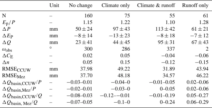
Table 3. Group average statistics of hydro-climatic changes for 4 groups of basins (“no change”, “climate only”, “runoff only” and “climate
& runoff”), classified by results of a combination of two-sample t-test results grouping basins with significant change atα=0.05. For the hydro-climatic changes, also the group standard deviation is given. For the normalised basin changes, the first and third quartiles are given. In total 351 basins have been tested.
Unit No change Climate only Climate & runoff Runoff only
N – 160 75 55 61
Ep/P – 1.15 1.22 1.10 1.28
1P mm 50±24 97±43 113±42 61±21
1EP mm −8±14 −13±23 −8±18 −7±12
1Q mm 23±41 44±45 95±31 67±43
ωobs ◦ 300 286 337 2
1CE – 0.02 0.05 −0.04 −0.06
1n – 0.05 0.15 −0.12 −0.15
RMSECCUW mm 37.98 49.22 31.89 43.94
RMSEMez mm 37.70 48.18 34.57 46.22 1Qbasin,CCUW/P – −0.03–0.01 −0.04–0 −0.01–0.05 0.02–0.06 1Qbasin,Mez/P – −0.02–0.01 −0.03–0 0–0.05 0.02–0.06 1Qbasin,CCUW/Q – −0.08–0.03 −0.12–−0.01 −0.01–0.19 0.05–0.27 1Qbasin, Mez/Q – −0.07–0.05 −0.1–0 0–0.24 0.06–0.29
detected climatic changes (with a group average decrease in aridity of−10.2 %). Further analysis shows thatETstrongly increased with 6.2 % of the annual water balance. Also the catchment parameter n and CE show significant increases (cf. Table 3). In contrast, the “runoff only” group shows sig-nificant positive basin change impacts (Budyko 3.8 % and CCUW 3.2 % of the annual water balance). In these basins, we find predominant increases in streamflow, along with sig-nificantly decreasing catchment parameters. This indicates that changes in the basin properties took place, which led to predominant runoff increases (7.7 % of the water balance) on similar magnitude of the group average precipitation in-crease (7.3 %). Thus, on average, the inin-crease in precipitation did not increaseET(−0.4 % of the water balance).
The “climate & runoff” change group reveals smaller er-rors; however, most of these tend to be influenced by basin changes with positive differences. The map in Fig. 4d dis-playing the location of the groups shows that many of these basins are actually close to the “runoff only” group and so we expect that basin changes are quite likely.
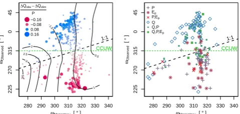
The ecohydrological framework of Tomer and Schilling (2009) is based on analysing changes in the relative parti-tioning of the surface water and energy fluxes. In Fig. 7, we plot the observed changes, i.e.1U vs.1W, using data of all MOPEX basins. From the figure, it becomes apparent that most of the basins shifted towards the right of the pos-itive diagonal, which is an effect of the general trend of in-creasing humidity (inin-creasingP and widely decreasingEp) over the US. The differences of the predicted changes to the observed changes in streamflow are depicted by the size of the dots and the colour palette. Generally, the smallest devia-tions are found in the lower right quadrant, which represents the climate impact change direction of the ecohydrological
concept. Towards the upper right quadrant, we find that basin impacts are increasing, leading to an excess of streamflow, while towards the lower left quadrant basin impacts show compensating effects leading to streamflow deficits.
In the right panel of Fig. 7, we use the plotting characters corresponding to the t-test classification groups. Most basins in the “runoff only” group are in the upper right quadrant, while the “climate only” group is concentrated in the lower two quadrants and predominant1U increases. So, although the concept of Tomer and Schilling has certain limitations such as the dependency to the aridity index and the hydro-logical response (Renner et al., 2012), it is generally able to separate the basin and climate impacts onETand streamflow. In summary, the analysis shows that the differences 1Qobs−1Qclimare unlikely to be random and due to model deficiencies, but rather reveal distinctive impacts of basin changes under the general trend of increasing humidity. Fur-ther, frequency and impacts of basin changes are large and evidently much larger than the differences between both frameworks.
4.3.4 Change direction in UW space