Innovative Algorithms and Evaluation Methods for Biological Motif Finding

Mathematics Theses Department of Mathematics and Statistics

Spring 5-1-2012

Confidence Interval Estimation for Coefficient of Variation

Confidence Interval Estimation for Coefficient of Variation

Shuang Liu

Follow this and additional works at: https://scholarworks.gsu.edu/math_theses

Recommended Citation Recommended Citation

Liu, Shuang, "Confidence Interval Estimation for Coefficient of Variation." Thesis, Georgia State University, 2012.

https://scholarworks.gsu.edu/math_theses/124

This Thesis is brought to you for free and open access by the Department of Mathematics and Statistics at ScholarWorks @ Georgia State University. It has been accepted for inclusion in Mathematics Theses by an authorized administrator of ScholarWorks @ Georgia State University. For more information, please contact

by

SHUANG LIU

Under the Direction of Dr. Gengsheng Qin

ABSTRACT

The coefficient of variation (CV) is a helpful quantity to describe the variation in

eval-uating results from different populations. There are many papers discussing methods of

constructing confidence intervals for a single CV, such as exact method and approximation

methods for CV when the underlying distribution is a normal distribution. However, the

exact method is computationally cumbersome, and approximation methods can’t be applied

when the underlying distribution is unknown. In this thesis, we propose the generalized

confidence interval for CV when the underlying distribution is normal and three empirical

likelihood-based non-parametric intervals for CV when the underlying distribution is

un-known. Simulation studies are conducted to compare the relative performances of these

intervals based on the coverage probability and average interval length. Finally, the

appli-cation of the proposed methods is demonstrated by using some real examples.

by

SHUANG LIU

A Thesis Submitted in Partial Fulfillment of the Requirements for the Degree of

Master of Science

in the College of Arts and Sciences

Georgia State University

by

SHUANG LIU

Committee Chair: Dr. Gengsheng Qin

Committee: Dr. Xin Qi

Dr. Xu Zhang

Electronic Version Approved:

Office of Graduate Studies

College of Arts and Sciences

Georgia State University

ACKNOWLEDGEMENTS

First and foremost, I would like to sincerely thank my advisor, Dr. Gengsheng Qin, for

all his help and guidance. Without his support, advice and patience, this thesis would not

have been possible to accomplish. I feel very lucky to be one of Professor Qin’s student.

And I would like to thank other thesis committee members, Dr. Xin Qi and Dr. Xu

Zhang, for taking their precious time out from their busiest and important moment and

giving helpful suggestion to my thesis work. I would also like to show my gratitude to some

of my classmates studying in similar field, Binhuan Wang, Haochuan Zhou and Aekyung

Jung, for their unselfish help and support. In addition, I would like to thank those who have

been traveling in the statistical world with me, my other classmates Hanfang Yang, Shan

Luo, Hongwei Wang, Zhu Zi for their encouragement. And I also want thank Ruya Zhao

who has been always supporting and understanding.

Lastly, I owe my deepest gratitude to my parents who have been supporting and

encour-aging me with all their hearts in all the ways. I couldn’t have achieved any success without

TABLE OF CONTENTS

ACKNOWLEDGEMENTS . . . iv

LIST OF TABLES . . . vi

CHAPTER 1 INTRODUCTION . . . 1

1.1 Background . . . 1

1.2 Parametric inference on Coefficient of Variation . . . 2

1.3 The purpose of the present study . . . 6

CHAPTER 2 METHODOLOGY . . . 7

2.1 Existing method . . . 7

2.2 New Methods . . . 10

2.2.1 Generalized Confidence Interval . . . 10

2.2.2 Empirical likelihood based method . . . 13

2.2.3 Jackknife Empirical Likelihood Method . . . 18

CHAPTER 3 SIMULATION STUDIES . . . 22

CHAPTER 4 REAL EXAMPLE . . . 31

CHAPTER 5 DISCUSSION AND CONCLUSION . . . 34

LIST OF TABLES

Table 3.1 The coverage probability and average length of 90 percent, k = 0.2,

Underly distribution :Normal . . . 25

Table 3.2 The coverage probability and average length of 90 percent, k =

0.5,underly distribution: normal . . . 26

Table 3.3 The coverage probability and average length of 90 percent, k =

1,underly distribution: normal . . . 27

Table 3.4 The coverage probability and average length of 90 percent, k =

0.2,underly distribution: Chi-square . . . 28

Table 3.5 The coverage probability and average length of 90 percent, k =

0.5,underly distribution: Chi-square . . . 29

Table 3.6 The coverage probability and average length of 90 percent, k =

1,underly distribution: Chi-square . . . 30

Table 4.1 The 90 percent Confidence Interval and Exact Length for CV of

Av-erage value of products sold (thousands) . . . 33

Table 4.2 The 90 percent Confidence Interval and Exact Length for CV of

CHAPTER 1

INTRODUCTION

1.1 Background

The coefficient of variation (CV) is an important quantity to describe the variation. It

provides an alternative index besides the most commonly used measurements of variation

such as variance or standard deviation, which come across with difficulty in comparing the

variations from different populations with different units. Take the data from students

physical examination as an example. If one wants to analyze variations of both height and

weight, it is not appropriate and logically incorrect to directly compare the variances or

standard deviation, as the units from both populations are not matched. Another practical

example in which commonly used measurements of variation might fail to work properly

is to describe the relationship between the variation of average individual income and the

variation of tax income of States. The different scale of data makes the direct comparison

invalid or misleading. Nevertheless, With the property of standardization and unitlessness,

CV makes the comparison possible. It is a good measure of the reliability of the experiment,

which is, the smaller the CV values, the higher is the reliability of experiment (Gomez and

Gomez, 1984; Steel and Torrie, 1980). Hence, CV is frequently provided by researchers,

especially those in agricultural fields, in major publications. It is as well widely applied to

Let X be a random variable with mean µand variance σ2_{. The population coefficient}

of variation is defined as follows:

k= σ

µ

Assuming that observationsXi, i=1, 2, ..., n, are the independent identically distributed

sample from N(µ,σ) . The sample mean ¯X and sample variance S2 are the unbiased point

estimates of µand σ2_{, respectively. An estimator of parameter k is}

K = S_¯

X,

where ¯X = _n1 P

Xi, andS2 =

P

(Xi−X¯)2 n−1 .

1.2 Parametric inference on Coefficient of Variation

CV does not appear to be the top mentioned index to measure the variation. Therefore,

not those like standard deviation or variance which has no secret of anything at all, there

aren’t many papers published about the inference of CV. However, the helpful application

of the index in the agricultural research and engineering field still drew some attention from

statisticians. And some authors have already done some impressive work for the inference of

of CV is given by Hendricks and Robey (1936) as follows,

dFcv =

2

π12Γ(n−1

2 )

e

− n 2σ_µ2

cv2

1+cv2 cvn−2

(1 +cv2₎n2 n−1

X

i=0

(n−1)!Γ(n−₂i) (n−1−i)!i!

ni2

2i2(σ µ)i

1 (1 +cv2₎2i

dcv.

Lehmann (1986) also derived the sample distribution of CV in order to give an exact

method for the construction of a confidence interval for CV. Suppose Xi are identically and

independently distributed from a normal distribution with mean µand variance σ2_{, then}

¯

X S

√

n

∼N CTn−1(

µ√n σ ),

where N CTn−1(µ

√

n

σ ) denotes a noncentral t-distribution with n-1 degrees of freedom and

non-centrality parameter µ

√

n

σ . With this distribution function, the confidence interval of

CV can be developed with standard procedure, yet with cumbersome calculation.

Routinely constructing an exact confidence interval for CV appears to be with difficulty

thanks to the complexity of distribution function. Thus, statistician chose to sacrifice certain

level of accuracy and proposed some simpler but relatively accurate approximation methods.

McKay (1932) first published the approximation method for constructing confidence

inter-val for CV under normal assumption. Based on the McKay’s work, David (1949) proposed

method is selecting an appropriate pivot quantity, he proved that by selecting a very simple

or “naive” approximate pivot, confidence interval for CV can be still obtained with

accept-able accuracy. Later, based on analysis of the distribution of a class of approximate pivotal

quantities, Vangel (1996) modified McKay’s method. He compared David’s (1949)

approxi-mation with Mckay’s (1932) and pointed out that the “naive” method resulted less accuracy

than McKay’s method. He then proposed his own approximation by extending McKay’s

(1932) method and obtained the result with satisfactory accuracy. The form of

approxi-mate pivotal quantities are presenting in the later chapter and the method of constructing

confidence interval for CV is given in the same chapter too.

Besides all the approximate pivotal quantity methods, Barndorff-Nielsen (1986, 1991),

Pierce and Peters (1992) and Reid (1996) proposed various likelihood based inference

pro-cedures which can be as well used to construct confidence interval for CV.

Let θ = (k, µ) , where k and µ are population CV and mean respectively, and let

l(θ) = l(k, µ) be the log likelihood function of θ. The Signed log-likelihood ratio statistics

for k is

r(k) =sgnd(ˆk−k)2[l(ˆθ)−l( ˆθk)] 1 2,

where ˆθ = (ˆk,µˆ) is overall maximum likelihood estimate of θ = (k, µ) and ˆθk = (k,µˆk)

is a constrained maximum likelihood estimate of θ for a given k . Then it can be proved

that r(k) is asymptotically following the standard normal distribution. Thus, the confidence

interval for k can be constructed. However, Pierce and Peters(1992) pointed out that this

sample size. A modified Signed log-likelihood ratio statistic was proposed by

Barndorff-Nielsen(1986,1991) as follows:

r∗(k) =r(k) +r(k)−1log{u(k)

r(k)}.

And he also showed that r∗ is asymptotically distributed with N(0,1) with accuracy of

O(n−32). In order to obtain the 100(1−α)% confidence interval, a simplified signed

log-likelihood ratio statistics is also given as

r(k) = sgnd(ˆk−k){2nlog(kµˆk ˆ

kµˆ ) +

n k2_µˆ2

k

[ˆk2µˆ2+ (ˆµ−µˆk)2]−n} 1 2,

where

ˆ

µk =

−y¯+py¯2_{+ 4k}2_(S2_{+ ¯y}2₎

2k2 , µˆ= ¯y

and

u(k) =√n{1

2+ 1 2(

ˆ

kµˆ

kµˆk

)2− µˆ

ˆ

µk

}( ˆ

kµˆ

kµˆk

)(1 +k2− µˆ

2ˆµk

Hence, with all the formulas above, r∗ can be easily obtained. Therefore, a 100(1−α)%

confidence interval for k is

CI ={k:|r∗(k)| ≤zα 2}.

1.3 The purpose of the present study

The goal of this thesis is to propose three new methods of constructing confidence

interval for CV. Comparison will be made with existing methods according to the coverage

probability and length of confidence interval. Methodology for different interval estimates

will be presented in detail in chapter 2 and adequate simulation work will be given to show

the performance of different interval estimates in Chapter 3. In Chapter 4 conclusion of this

CHAPTER 2

METHODOLOGY

2.1 Existing method

As mentioned in Chapter 1, the complication of distribution function for CV rises the

difficulty of routinely constructing exact confidence interval for CV with standard process.

In order to avoid the cumbersome calculation, many authors proposed relatively accurate

approximation methods. McKay (1932) first proposed the approximation method by using

the approximate pivotal quantity. And later David (1949) and Vangel (1996) gave the

modified methods based on different pivot quantity selections. Since the sufficient part of the

approximation method is selecting the appropriate pivot quantity, the detailed mathematical

procedure of Vangel’s (1996) work will be presented to illustrate the method.

LetYv be a random variable following the chi-square distribution with degree of freedom

v =n−1 , and define Wv = Y_vv. For any α ∈(0,1) , let χ2v,α denote the 100α percentile of

the distribution of Yv , then t = χ2

v,α

v is the corresponding quantile for Wv . Vangel (1996)

defined the random variable as follows:

Q= K

where θ = θ(k, α) is a known function, K = S

¯

Y is the sample CV where S

2 _{and ¯Y is the}

sample variance and sample mean respectively. Select a proper θ such that

P r(Q < t)≈P r(Wv ≤t).

The selection of θ is the most important part for the approximation method. The

approximation methods mentioned above basically were all trying to select an appropriate

θ. They are relatively simple but maintain relatively satisfactory accuracy. McKay (1932)

claims that the selection of θ = _v+1v would make a good approximation for Q. And David

(1949) gave an even simpler selection of θ which set θ= 1 . Another “naive” approximation

was proposed by setting θ = 1_t. Later Vangel (1996) proved that the distribution of Wv is

known and is free of K, and he proposed a modified θ with the expression of

θ = v

v + 1[ 2

χ2

v,α

In general, with the selected θ, the 100(1−α)% approximate confidence interval for k

is given as follows by using the approximate pivot:

CI = (_p K

t1(θ1K2+ 1)−K2

,_p K

t2(θ2K2+ 1)−K2 ),

where t1 =

χ2_v,1−α 2 v , t2 =

χ2_{v, α} 2

v , and θi =

2 (v+1)ti +

v

k+1, i = 1,2. So the McKay and Vangel’s

interval estimates are

CI1 ={K[(

u1

v+ 1 −1)K 2₊ u1

v ]

−1

2, K[( u2

v+ 1 −1)K 2₊u2

v ]

−1 2},

and

CI2 ={K[(

u1+ 2

v+ 1 −1)K 2₊u1

v ]

−1

2, K[( u2

v+ 1 −1)K

2₊u2+ 2

v ]

−1 2},

respectively, where ui ≡vti, fori= 1,2.

Although, by using the approximate pivot, one can obtain a confidence interval for

desired index with very satisfactory accuracy for some true values of k, the McKay and

Vangel’s methods come across some inevitable problem. With some simple calculation, one

can prove that the pivotal quantities may be a complex value when selecting a largek. That

that his methods could only be applied under the condition ofk < 0.33 (McKay, 1932). The

same drawback appears for Vangel’s method too. These unavoidable problems inspired us

for seeking some new methods introduced in next section.

2.2 New Methods

2.2.1 Generalized Confidence Interval

Inspiring by McKay(1932) and Vangel’s(1996) approximation methods which introduced

some pivotal quantities to construct the confidence interval, we are thinking about if it is

possible to propose a different type of pivotal quantity. Since lots of works about Generalized

Confidence Interval have been done based on Generalized Pivotal Quantity (GPQ) in the

literature, in this section, we proposed a method to develop a GPQ-based confidence interval

for CV. The definition of GPQ is as follows, cited from Weerahandi (1993):

Let X be an observable random vector with the cdfF(x|v), wherev = (θ, δ) is a vector of

unknown parameters,θis the parameter of interest, andδ is a vector of nuisance parameters.

Let χ be the sample space of possible values of X and let Θ be the parameter space of θ.

An observation from X is denoted by x, where x ∈ χ . Let R = r(X;x, v) be a function

of X, x, v (but not necessarily a function of all), where v = (θ, δ) . Then it is said to be a

generalized pivotal quantity if property A: R has a probability distribution free of unknown

parameters. Property B: The observed pivotal, defined as robs =r(x;x, v) , does not depend

on the nuisance parameter δ .

Then a two-sided 100(1−α/2)% confidence interval for parameterθ is (Rα/2, R1−α/2) ,

distribution R respectively. More detailed introduction of GPQ-based confidence interval is

referred to Weerahandi (1993) and Hanning et al. (2006).

Now let observationsX1, ..., Xm be the random sample from a normal distribution with

mean µ and standard deviation σ . Then the sufficient estimator for (µ, σ) is

(ˆµ,σˆ) = ( ¯X, S)

where ¯X = _m1 Pm

i=1Xi, and S

2 ₌ Pmi=1(Xi−X¯) m−1 .

Under normality assumption, the parameter of interest D is a function of parameters

(µ, σ) which is

(µ, σ2, k) = (µ, σ2,σ µ).

So the parameter can be estimated by

(ˆµ,σˆ2,ˆk) = ( ¯X, S2, S_¯ X)

Let U ,Z be the quantities defined as follow:

U = (n−1)S 2

σ2 ∼χ 2

Z = (σ 2

n )

−1/2_{( ¯X−µ)∼N(0,1).}

And we can easily verify that both properties A and B are satisfied in these quantities.

Therefore, defined quantities are the pivotal quantities corresponding to estimators.

Let ¯x and s2 be the observation of ¯X,S2 respectively. Then the GPQ ofσ2,and µis in

expression of

R_σ2 =

(n−1)s2

U , (2.1)

and

Rµ= ¯x−( Rσ2

n )

1/2_{Z. (2.2)}

Based on this, the GPQ for the parameter of interest k is expressed as

Rk=

√

Rσ2 Rµ

. (2.3)

To construct a GPQ-based confidence interval with given observations x1, ..., xm from

N(µ, σ2), we propose the following Monte-Carlo algorithm:

STEP 1: Compute the sample mean and sample standard deviation using original

observation samples.

STEP 2: Randomly generate one U from corresponding chi-squared distribution with

STEP 3: Calculate R_σ2,R_µ by using (2.1) and (2.2).

STEP 4: Calculate Rk by using (2.3).

STEP 5: Repeat STEP2-STEP4 H times (10000 times is recommended) to obtain H

values of Rk .

Consequently, the 100(1−α)% GPQ-based confidence interval for CV can be obtained

as (Rk,α/2, Rk,1−α/2) , where Rk,α/2 and Rk,1−α/2 are the 100(α/2)−th and 100(1−α/2)−th

percentiles of Rk’s.

2.2.2 Empirical likelihood based method

Parametric methods of obtaining confidence interval for CV have been discussed and

improved by many authors over the past several decades as we mentioned above. When the

underlying distribution is a normal distribution, one is well-equipped of several methods to

construct a confidence interval for CV. Nevertheless, in practice, the normality assumption

may not be easily guaranteed. In these cases, which happen quite frequently, those methods

are performing poorly or even invalid. Then it is really crucial to introduce a non-parametric

method to compensate the incompletion of existing methods.

When addressing the non-parametric method for constructing confidence intervals,

Owen (1988, 1990) is the one who must be mentioned, because he proposed a very

pow-erful non-parametric method for constructing confidence interval for parameters of interest,

which is well-known as Empirical likelihood (EL). With a lot of advantages, EL method was

in the center of attention once the method purposed and has been widely applied to many

piv-otal statistic; 2. No prior constraints of the shape of confidence region is needed; 3. it may

confesses a Bartlett correction that tolerates low coverage error. More detailed information

on EL method can be refereed to Hall and La Scala (1990). However, the EL-based method

for CV has not been well-developed. So, in the following paragraph, we attempt to apply

the empirical method to the construction of confidence intervals for CV.

Recall that

k =

p

E(X2_)−(E(X)2₎

E(X)

is a smooth function of the mean m = (E(X), E(X2)). Owen (1988) showed that the

limiting distribution of the empirical log-likelihood ratio for m is a chi-square distribution

with 2 degree of freedom. Hence, an EL-based joint confidence region for mcan be obtained

from the chi-square distribution, and an EL-based confidence interval for the CV can be

found based on this confidence region. This is the original idea from Owen (1988) and an

indirect way to construct confidence interval for the CV. However, this method involves in a

2-dimensional confidence region and it is somewhat uncomfortable in implementation. Thus,

here we proposed a plugging-in EL method for constructing confidence interval of the CV.

We observe that the coefficient of variation k satisfies the following equation:

Let P = (p1, ..., pn) be a probability vector. Then the EL for k can be defined as follows:

L(k) =su Pp{

n

Y

i=1

pi :pi ≥0, n

X

i=1

pi = 1, n

X

i=1

piWi = 0},

whereWi =σ−kXi, i= 1,· · · , n. Since parameterσ is unknown in practice, we use sample

standard deviation S to estimate it. Then, the profile EL fork can be defined as follows:

ˆ

L(k) =su Pp{

n

Y

i=1

pi :pi ≥0, n

X

i=1

pi = 1, n

X

i=1

piWˆi = 0},

where ˆWi =S−kXi .

With Lagrange multiplier method, we can obtain the expression for pi , which is

pi =

1

n{1 +λ

ˆ

Wi}−1, i= 1, ..., n,

where λ is the solution to

1 n n X i=1 ˆ Wi

1 +λWˆi

Therefore, the profile EL ratio for k is:

R(k) =

n

Y

i=1

(npi) = n

Y

i=1

{1 +λWˆi}−1.

Then the corresponding empirical log-likelihood ratio for k is

l(k) = 2

n

X

i=1

log{1 +λWˆi}, (2.4)

where λ is the solution of the equation _n1 Pn

i=1 ˆ

Wi

1+λWˆi = 0. Following Theorem 2.1 in Hjort

et al. (2009), we find out that l(k) actually asymptotically follows a scaled chi-square

distribution.

Theorem: If k is the true value of the coefficient of variation, then the limiting

distri-bution of l(k), defined by (3), is a scaled chi-square distribution with degree of freedom one.

i.e. ,

cl(k)−→d χ2₁,

where the scale constant is c≈ 1

Since c is an unknown constant, in order to construct confidence interval for the CV

based on this theorem, we have to estimate c. Here we propose the following bootstrap

procedure to estimate the scale constant.

Step 1: generate bootstrap sample X₁∗,· · ·, X_n∗ from the original sample X1,· · ·, Xn.

Step 2: find the bootstrap estimate l∗(ˆk) ofl(k):

l∗(ˆk) = 2

n

X

i=1

log{1 +λ∗Wˆ_i∗}

where ˆW_i∗ =S∗−kXˆ _i∗ is the bootstrap version of ˆWi, ˆk is the sample coefficient of variation

from the original sample, and λ∗ is the solution of

1

n n

X

i=1 ˆ

W_i∗

1 +λ∗_Wˆ∗

i

= 0.

Step 3: repeat steps 1-2 B times (B ≥ 200 is recommended) to obtain B bootstrap

copies of l(k):

Step 4: Estimate the constant c as follows:

c∗ = [1

B n

X

i=1

l∗_i(ˆk)]−1

Based on Theorem and the estimated constant c∗, we can construct the bootstrap

EL-based confidence interval (BEL interval) for k as follows:

{k :c∗l(k)≤χ2₁(1−α)}

where χ2

1(1−α) is the (1−α)−th quantile of χ21 .

2.2.3 Jackknife Empirical Likelihood Method

In previous section, we introduced the bootstrap EL-based confidence interval (BEL

interval). Despite of all the advantages the method has, serious computational difficulty is

inevitably occurred, as well as one has to estimate the constant coefficientcfor the scaled

chi-square distribution, which may introduce extra bias. Recently, Jing, Yuan and Zhou (2009)

raised a new approach called jackknife empirical likelihood (JEL) method. The logarithm

of the Jackknife empirical likelihood ratio asymptotically follows the standard Chi-square

is extremely simple in calculation. In following context, we will develop the JEL-based

method to construct confidence interval for CV.

Let Xi, i = 1, ..., n be a random sample from a population with unknown underlying

distribution. The sample coefficient of variation can be calculated as follows:

ˆ

k = S_¯

X

The corresponding jackknife pseudo values are

ˆ

Wi =nkˆ−(n−1)ki, i= 1, ..., n

where ki is the sample coefficient of variation computed with (n−1) sample observations

after deleting i−th observation from the original sample.

With similar argument in Tukey (1958), ˆWi’s are expected to be asymptotically

inde-pendent. Then standard empirical likelihood methods could be applied to these jackknife

be a probability vector. The jackknife empirical likelihood for CV can be defined as follows:

LJ(k) =su Pp{

n

Y

i=1

pi :pi ≥0, n

X

i=1

pi = 1, n

X

i=1

pi(Wi−k) = 0}.

And just as previous section, the Lagrange multiplier method provides the Jackknife

empir-ical log-likelihood ratio:

lJ(k) = 2 n

X

i=1

log{1 +λJ(Wi−k)},

where λJ is the solution of the equation:

1

n n

X

i=1

Wi−k

1 +λJ(Wi−k)

= 0.

The Jackknife empirical log-likelihood ratio asymptotically follows a chi-square

distri-bution with 1 degree of freedom. i.e.,

lJ(k) d

Therefore, the Jackknife empirical-based confidence interval fork can be constructed as

follows:

{k:lJ(k)≤χ21(1−α)}

where χ2

CHAPTER 3

SIMULATION STUDIES

Newly introduced methods need to be examined and we need to show more evidence to

illustrate the advantages of new methods over the existing ones. In this section, adequate

simulation studies have been conducted to give a clear comparison between newly proposed

confidence intervals and existing confidence intervals. The intervals being examined in the

simulation study are Vangel’s modified approximate method (Vangel), the Generalized

Piv-otal Quantity method (GPQ), Plug-in empirical likelihood with bootstrap-based confidence

interval (BEL) and the Jackkinfe empirical likelihood confidence interval(JEL).

Considering the practical application for agriculture and engineering fields, the finite

sample performance is the main issue we focus on. In the simulation studies, we carried

out the simulation with sample size n = 30,50,100,200, to examine the performance from

smaller sample size to larger sample size. According to the property of the coefficient of

variation, we selected the true value k = 0.2,0.5,1 to investigate the performance of all

methods mentioned above. Largek may result in a non-negligible probability of obtaining a

negative observation, and based on practical application, the scenario is of less interest. Thus

the selected true values are narrowed down to the range from 0 to 1. The iteration times

R = 1000 and bootstrap replication B = 200 were chosen for calculating BEL intervals

because of the computational extensiveness with bootstrap method, and R = 10000 was

Two underly distributions, normal distribution and Chi-square distribution, were selected

to generate the random observations. For the setting with normal distribution as the

pre-selected underly distribution, we consider all the methods mentioned above and make the

comparison. However, as k getting larger, the vangel’s method failed to work properly due

to the property of the pivotal quantity. We mark N/A as comparing the rest. In the other

setting, Chi-square distribution was selected as the underly distribution to examine the

proposed non-parametric approaches. Since the normality assumption is invalid, Vangel and

GPQ can not be applied to the setting.

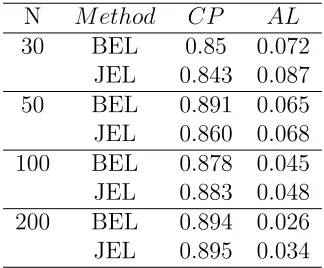
We calculated the coverage probability (CP) and average length (AL) as the criteria

to evaluate the performance of these intervals. At the nominal confidence level 90%, we

calculated the percentages that the confidence intervals cover the true value of k. The closer

the percentage is to the nominal level, the better performance of the confidence interval.

Average length (AL) is the summation of all length of confidence intervals divided by total

number of iteration. With similar coverage probabilities, the shorter average length is, the

better performance of the confidence interval. All the simulation studies were conducted

with the statistical package R.

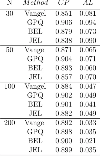
The simulation results are displayed in table 3.1 to table 3.6 . From table 3.1, we

conclude that GPQ interval has the best performance among the four intervals regardless

the sample size in this scenario. Its coverage probabilities are very close to the nominal level.

Vangel, BEL and JEL intervals undercover the true value with small to moderate sample sizes

(n = 30,50,100), but they are acceptable as sample sizenincreases to 200. Vangel’s method

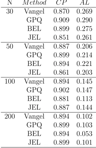
Table 3.2 shows the similar performances for all the methods as we selected k = 0.5. As k

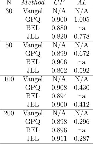
getting larger, the average lengths increase. Table 3.3 shows the simulation results fork = 1.

Due to the property of approximate pivotal, Vangel’s method is not available (N/A). And

the proposed methods still perform with satisfactory, especially the GPQ method. Tables

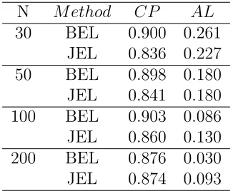
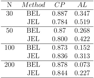
3.4 to 3.6 are the results from the setting of non-normality assumption. With the Chi-square

distribution as the underly distribution, GPQ and Vangel’s methods are no longer valid,

but we can apply the proposed non-parametric methods. The results show that, BEL and

JEL undercover the true values of k with small to moderate sample sizes (n = 30,50,100).

However, as sample size increases, the coverage probabilities are approaching to the nominal

level. Among different k values in this setting, BEL performs slightly better than JEL in

terms of coverage probability.

In sum, under normality assumption, GPQ has the best performance with the

appro-priate coverage probability and stability. Comparing to the existing method, GPQ is more

powerful as it expands the range of availability for the value of coefficient of variation. We

recommend GPQ when the underly distribution is normal. Under non-normality

assump-tion, the performances of the JEL and BEL intervals are acceptable when sample size is

big enough. Therefore, JEL and BEL are recommended when the underlying distribution is

Table 3.1. The coverage probability and average length of 90 percent,k = 0.2, Underly distribution :Normal

N M ethod CP AL

Table 3.2. The coverage probability and average length of 90 percent, k= 0.5,underly distribution: normal

N M ethod CP AL

Table 3.3. The coverage probability and average length of 90 percent, k= 1,underly distribution: normal

N M ethod CP AL

30 Vangel N/A N/A GPQ 0.900 1.005

BEL 0.880 na JEL 0.820 0.778 50 Vangel N/A N/A

GPQ 0.899 0.672 BEL 0.906 na

JEL 0.862 0.592 100 Vangel N/A N/A

GPQ 0.908 0.430 BEL 0.894 na

JEL 0.900 0.412 200 Vangel N/A N/A

GPQ 0.898 0.296 BEL 0.896 na

Table 3.4. The coverage probability and average length of 90 percent, k= 0.2,underly distribution: Chi-square

N M ethod CP AL

Table 3.5. The coverage probability and average length of 90 percent, k= 0.5,underly distribution: Chi-square

N M ethod CP AL

Table 3.6. The coverage probability and average length of 90 percent, k= 1,underly distribution: Chi-square

N M ethod CP AL

CHAPTER 4

REAL EXAMPLE

In this chapter, a real case is studied to illustrate the methods we introduced in the

previous chapters. The practice sample data set named Beef Council Check-off is obtained

from The Data and Story Library (DASL) at Carnegie Mellon University. Among 7 variables

in the data set, we chose 2 of them to conduct the experiment, Average size of farm (hundreds

of acres) and Average value of products sold (thousands). Each of the variable contains 56

observations, which is similar amount as moderate sample size we chose to conduct the

simulation study.

In order to check the normality of each variable, the normality test called Shapiro-Wilk

test has been conducted. The null hypothesis of Shapiro-Wilk test is that sample data

x1, x2, ..., xn is from normal distribution. The small p-value (smaller than the significant

level one selected) indicates the rejection of null hypothesis which means the sample data

is from non-normal distribution. And if one fails to reject the null hypothesis, we can treat

the sample data comes from normal distribution. More detailed information can be referred

to Shapiro and Wilk (1965).

For variable of average value of products sold (thousands), the sample coefficient of

variation ˆk = 0.4733. And regarding to Shapiro-Wilk test, the calculated p-value is 0.5037

which indicates that sample data is from a normal distribution. Based on the test results, we

for CV. Table 4.1 shows the simulation results. From Table 4.1, we can see that confidence

intervals calculated from all mentioned methods are very similar. We can conclude that BEL

and JEL are relatively better due to the slightly shorter Exact Length.

Similarly, the sample coefficient of variation for variable of average size of farm (hundreds

of acres) is ˆk = 0.6594. Shapiro-Wilk test was conducted to test the normality. With

calculated p-value 0.002981,the null hypothesis is rejected at the significant level of 0.05,

which indicates the sample is from a population with non-normality distribution. Therefore,

we can only apply the newly proposed non-parametric methods to calculate the confidence

interval for CV with the nominal level 0.9. The simulation results can be found in Table 4.2.

Table 4.1. The 90 percent Confidence Interval and Exact Length for CV of Average value of products sold (thousands)

Method Confidence Interval Exact Length Vangel (0.3986, 0.5755) 0.1769

GPQ (0.3973, 0.5872) 0.1898 BEL (0.4068, 0.5606) 0.1538 JEL (0.4067, 0.5579) 0.1512

Table 4.2. The 90 percent Confidence Interval and Exact Length for CV of Average size of farm (hundreds of acres)

Method Confidence Interval Exact Length BEL (0.5858, 0.7726) 0.1869

CHAPTER 5

DISCUSSION AND CONCLUSION

The significance of the coefficient of variation may be underestimated by statisticians.

Comparing to other frequently mentioned indexes for variation, CV draws less attention

from statisticians. However, with the properties of unitlessness and mean-related,

coeffi-cient of variation appears more and more in applied researches such as agriculture field and

engineering field. In literature, several methods of constructing confidence interval for CV

have been introduced in the past decades. Nevertheless, most of existing methods are of

deficiency. The dependency of underlying distribution and narrowed availability range for

CV are the main motivation for this thesis study. In this thesis, we proposed a new

para-metric interval and two non-parapara-metric intervals for CV. Under the normality assumption,

the GPQ-based confidence interval shows a nearly perfect small sample performance, and

successfully extend the availability range for CV. Therefore, it is recommended to use

GPQ-based confidence interval for CV under normality assumption. Through plenty of simulation

studies, the BEL and JEL confidence intervals are shown to have acceptable finite sample

performances when sample size is big enough ( n ≥ 200). Since they are non-parametric

intervals, they are particularly useful to obtain confidence intervals for CV from the

popu-lation with non-normality assumption. Thus, these non-parametric methods are suggested

to obtain confidence intervals for the coefficient of variation with unknown underlying

shown in the simulation study when sample size is small. The future research will focus on

REFERENCES

[1] Barndorff-Nielsen, O.E. (1986), Inference on full or partial parameters based on the

standardized Signed log-likelihood ratio, Biometrika 73: 307-322.

[2] Barndorff-Nielsen, O. E. (1991). Modified Signed log-likelihood ratio. Biometrika 78:

557-563.

[3] David, F. N. (1949). Note on the application of Fisher’s k-statistics. Biometrika 36:

383-393.

[4] Hanning, J., Iyer, H.K., and Patterson, P.. (2006). Fiducial Generalized Confidence

Intervals. Journal of the American Statistical Association, 101, 254-269.

[5] Hjort, N. L.., McKeague, I. W. and Keilegom, I. V. (2009). Extending the scope of

empirical likelihood. Ann. Statistics 37, 1079-1111.

[6] Girma Taye and Peter Njuho (2008). Monitroing Field Variability Using Confidence

Interval for Coefficient of Variation, Communications in Statistics-Theory and Methods,

37: 831-846.

[7] Gomez, K. A., Gomez, A. A. (1984). Statistical Procedures for Agricultural Research.

2nd ed. New York: John Wiley and Sons, Inc.

[8] Hall P. and La Scala B. (1990), Methodology and Algorithms of Empirical Likelihood,

[9] Jing B., Yuan J. and Zhou W. (2009), Jackknife Empirical Likelihood, Journal of the

American Statistical Association, Vol.195, No. 487, pp. 1224-1232.

[10] Johnson, N. L., Welch, B. L. (1940), Application of the no- central t-distribution.

Biometrika 31: 362-389.

[11] Lehmann, E. L. (1986), Testing Statistical Hypothesis. 2nd ed. New York: Wiley.

[12] Loh W. (1991) , Bootstrap calibration for confidence interval construction and selection,

Statistica Sinika, Vol.1, pp. 477-491.

[13] McKay, A. T.(1932). Distribution of the coefficient of variation and the exextended

t-distribution. J. Roy. Statist. Soc. B 95: 695-698.

[14] Owen A.B. (1988), Empirical likelihood ratio confidence intervals for a single functional,

Biometrika, Vol.75, pp. 237-249.

[15] Owen A.B. (1990), Empirical likelihood ratio confidence regions, Biometrika, Vol.18,

pp. 90-120.

[16] Peter Sprent and Nigel C. Sweeton (2007), Applied Nonparametric Statistical Methods,

Chapman Hall/CRC, fourth edition.

[17] Pierce, D. A., Peters, D. (1992). Practical use of higher order asymptotic for

multipa-rameter exponential families (with discussion). J.Roy. Statist. Soc. B 54:701-738.

[18] Qin, G.S., and Zhou, X.H. (2006), Empirical likelihood inference for the area under the

[19] Qin J. and Lawless J. (1994), Empirical likelihood and general estimating equations,

The Annals of Statistics, Vol. 22, No.1, pp. 300-325.

[20] Reid, N. (1996), The roles of conditioning in inference. Statist. Soc. B 54: 701-738.

[21] Shapiro, S. S.; Wilk, M. B. (1965). An analysis of variance test for normality (complete

samples). Biometrika 52 (3-4): 591C611.

[22] Steel, R. G. D., Torrie, J. H. (1980). Principles and Procedures of Statistics, 2nd ed.

New York: McGraw-Hill.

[23] Tukey, J. W. (1958). Bias and confidence in not-quite large samples. Ann. Statist. 29,

614.

[24] Vangel, M. G. (1996). Confidence intervals for a normal coefficient of variation. Am.

Statist. 50: 21-26.

[25] Walter A. Hendricks and Kate W. Robey (1936) . The Sampling Distribution of the

Coefficient of Variation. Ann. Math. Statist. Vol. 7, No. 3, pp.129-132.

[26] Weerahandi S. (1993), Generalized confidence intervals, Journal of the American