item and our policy information available from the repository home page for further information.
Author(s):Chanerley, Andrew A; Alexander, Nick
Title:A brief review of instrument de-convolution of seismic data Year of publication:2006
Citation:Chanerley, A.A., Alexander, N. (2006) ‘A brief review of instrument de-convolution of seismic data’ Proceedings of Advances in Computing and Technology, (AC&T) The School of Computing and Technology 1st Annual Conference, University of East London, pp. 95-101
Link to published version:
A BRIEF REVIEW OF INSTRUMENT DE-CONVOLUTION
OF SEISMIC DATA
Andrew A Chanerley, Nick Alexander
* Built Environment Research Group*Bristol University, Department of Civil Engineering [email protected], [email protected]
Abstract: Most corrected seismic data assume a 2nd order, single-degree-of-freedom (SDOF)
instrument function with which to de-convolve the instrument response from the ground motion. Other corrected seismic data is not explicitly de-convolved, citing as reason insufficient instrument information with which to de-convolve the data. Whereas this latter approach may facilitate ease of processing, the estimate of the ground motion cannot be entirely reliable and therefore methods of de-convolution have been suggested and described in [1, 2, 4 ,5]]. This paper reviews a relatively straightforward implementation of the well-known recursive least squares (RLS) algorithm in the context of a system identification problem [4]. The paper then goes on to discuss the order in which implementation of the RLS algorithm should be applied when correcting seismic data. Noise reduction is typically achieved by de-noising using the discrete wavelet transform [8, 9] or filtering the resulting de-convolved seismic data. De-noising removes only those signals whose amplitudes are below a certain threshold and is not therefore frequency selective. Standard band-pass filtering methods on the other hand are frequency selective, but different cut-off frequencies for band-pass filters are applied in different parts of the world when correcting seismic events. These give rise to substantial differences in power spectral density characteristics of the corrected seismic data.
1. Introduction
Basic data for earthquake engineering is obtained from measurements of ground shaking during earthquakes. The first accurate measurements of destructive earthquake ground motions were made during the Long Beach, California earthquake of 10/03/33. Since then, considerable improvement have been made in strong motion instrumentation and measurements. Analogue systems are the simplest devices that are reasonably cheap to manufacture and require minimal maintenance. However data from these instrument require considerable data-processing time. Studies suggest that digital instruments on the other hand, although more expensive to maintain, provide a more accurate determination of ground motion and reduce data-processing time. Although
good progress has been made in replacing old instruments with digital ones, the vast majority of data currently available have been recorded from analogue instruments such as the SMA-1. Seismic data is sampled over the duration of an earthquake in the form of accelerograms. The accelerometer records acceleration as a function of time. In fact the output is the response of the instrument to the ground motion being measured. The data is inevitably smeared with background noise in both the short and long frequency range. Appropriate signal processing techniques are therefore necessary to extract acceleration data in order to mimic the actual ground motion.
2. Instrument de-convolution
applied because the header of the original data does not provide any information on useful instrument parameters or indeed the type of instrument used. In a lot of cases the seismic data analysed did not, after processing without instrument de-convolution, produce marked differences in outputs when processed with instrument de-convolution. However, with some data analysed the differences in outputs, in particular for the acceleration response spectra were clear and not insignificant. In most of the older records the accelerograms recorded the characteristics of strong-motion earthquakes with single-degree-of-freedom, stiff and highly damped transducers whose relative displacement x(t) is approximately proportional to the ground accelerationa g (t ) . To obtain estimates of the ground acceleration from the recorded relative displacement response, an instrument correction can be applied as follows:
) ( ) ( 2 ) ( )
(t x t x t 2x t
ag =−&& − γω& −ω (1) where γ = viscous damping ratio
ω= transducer natural frequency and ag (t) is the ground acceleration The above expression (1) can be used to de-convolve the recorded motion from the ground acceleration in either the time [6] or frequency domain [1]
3. De-convolution using the RLS
algorithm
The usefulness of this method resides in the fact that an estimate of the filter coefficients, which describe the instrument response, may be obtained from the seismic data set itself without any prior knowledge of the actual instrument used. Since quite often instrument data does not accompany the seismic data, then this method is a relevant
implementation because of course each data set reflects the individual instrument response to some degree. The other methods described above apply a one-size-fits-all approach.
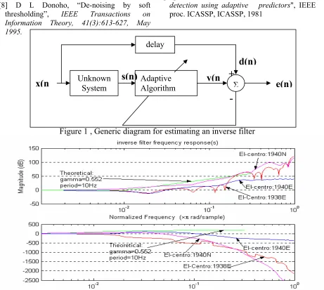
The generic algorithm for the inverse filter (system identification) problem using the Recursive Least Squares (RLS) algorithm is shown below in. This schemeapplies to any adaptive algorithm, with the unknown system cascaded with a particular adaptive algorithm; the solution converges to the inverse of the unknown system. The delay is added to keep the system casual so that the input data, s(n), has sufficient time to reach the adaptive filter. Otherwise it tries to minimise the error before the data s(n) has reached the adaptive algorithm and can never converge. The RLS algorithm [4,10,11,12] was chosen in preference to the least mean squares (LMS) adaptive algorithm. One reason is that the RLS algorithm is dependent on the incoming data samples rather than the statistics of the ensemble average as in the case of the LMS algorithm. Therefore the coefficients will be optimal for the given data without making any assumptions regarding the statistics of the process. Another reason is that the RLS algorithm converges at a faster rate than the LMS. The RLS algorithm can be considered in terms of a least squares solution [10] of the system of linear equations Ah = d, where rank A is n, the number of unknowns. The objective is to find the vector (or vectors) h
of filter coefficients which will satisfy equation (1). This has the well-known solution equations (2), (3) and (4).
{
2}
minimise Ah−d (2)
( )
A A A dh= T −1 T (3)
( )
G A d PA d h= −1 T = T(4) However in order to obviate the need of
auto-correlation matrix P, the RLS algorithm provides an efficient method of updating the least squares estimate of the inverse filter coefficients as new data arrive.
However the RLS algorithm can become numerically unstable and indeed with some seismic data does just that. Therefore a variant of the RLS algorithm is used in this paper which, for a given value of λ, reduces the dynamic range and leads to stable solutions in most cases. This is the QR decomposition-based RLS algorithm deduced from the square-root Kalman filter counterpart [10,11]. The square root is in fact a Cholesky factorisation and the derivation of this algorithm depends on the use of an orthogonal triangulation process known as QR decomposition.
= = r r r r r r r r r r 0 0 0 0 0 0 R
Q.A (5)
Where R is an upper triangular matrix and Q
is a unitary matrix and A is a data matrix. The QR decomposition of a matrix requires that certain elements of a vector be reduced to zero. The unitary matrices used zero out the matrix elements of A one-by-one or column-by-column and leaves an upper triangular matrix. It zeros out the elements of the input data matrix elements and updates the (square root) inverse correlation matrix. The QR-RLS is given in equation (6); where γk is a scalar.
= = − − − − − − 22 21 12 11 2 1 2 / 1 2 / 1 2 1 1 2 / 1 2 1 1 2 / 1 0 0 1 R P P P Q r r r k u T / k k k T k / k / k T k γ γ λ λ (6) The gain vector kk is determined from the 1st column of the post-array. Qk in the above expression is a unitary transformation which operates on the elements of
2 1 1 2 / 1 / k T u − − P
λ and the rows of 1 2 1 2 / 1 / k− − P
λ in the pre-array zeroing out each one to give a zero-block entry in the post-array. The least-squares weight vector, hk is updated in equation (9), but through equation (7) the gain vector, from the post-array equation (6), and equation (8) the a priori estimation error.
1 11 21
−
=
r
r
k
k (7)k T k k
k
=
d
−
h
−1u
ε
(8)k T k k
k
h
k
h
=
−1+
ε
(9)These inverse-filter weights are then convoluted with the original seismic data in order to obtain an estimate of the true ground motion. As in the standard RLS, the inverse correlation matrix is estimated, prior knowledge is not required, i.e. the algorithm is independent of the statistics of the ensemble.
40-120dB, with the theoretical gain at approximately 80dB at half the sampling rate. These results demonstrate the usefulness of using the QR-RLS in order to de-convolve the instrument response without any prior knowledge of the instrument parameters
In using the RLS for instrument de-convolution it is necessary to review the order in the implementation of noise removal and the application of the inverse filter. In using the filtering/de-noising methods described below, Butterworth or Elliptic band-pass filters, wavelet de-noising, in conjunction with the standard 2nd order differential equation, it doesn’t make any difference to the output as to whether the filtering/de-noising is pre-or post- the instrument de-convolution. This is because the solution to the differential equation is the same in both situations, it is not an estimate based on corrupted or de-corrupted input data, and therefore necessarily the inverse filter response is always the same. This changes with the application of the RLS algorithm, because the estimate of the inverse filter is dependent on the input data, therefore whether it has been pre-filtered or not makes a difference. Noise errors should, as far as is possible, be removed before an RLS instrument correction is applied, since the resulting de-convolution may amplify the noise inherent in a seismic data set and distort the frequency response
4. Wavelet De-noising
This method is based on taking the discrete wavelet transform (DWT) [9] of a signal, passing the transform through a threshold [8], which removes the coefficients below a certain value, and then taking the inverse DWT in order to reconstruct a de-noised time signal. The DWT is able to concentrate most of the energy of the signal into a small
number of wavelet coefficients, after low-pass filtering with the appropriate filter weights depending on the selection of a wavelet basis. The dimensions of the wavelet coefficients will be large compared to those of the noise coefficients obtained after high pass filtering. Therefore thresholding or shrinking the wavelet transform will remove the low-amplitude noise in the wavelet domain and the inverse DWT will retrieve the desired signal with little loss of detail.
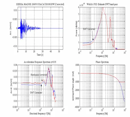
The Sierra Madre seismic event is shown in the plots of Figure 3. They show the low frequency detail on a log scale and clearly some differences between the two correction methods are again apparent. The PSD demonstrates that the large approximately 1Hz ground peak has had an insignificant impact on the structural frequency, whereas the smaller 5Hz-ground peak of the PSD has had a considerable impact on the structural frequency.
5. Summary
which it determines an estimate of the inverse of the instrument response. The point to emphasise however is that the standard 2nd order de-convolution is not necessarily a good reflection of instrument performance, but is probably better than not performing a de-convolution at all.
The order of events is also important because the data should be de-noised or filtered prior to the instrument correction. This is to prevent any amplification of noise during the de-convolution process. The results however do show that over frequencies of interest it is still possible to obtain approximately zero magnitude and phase response when de-convoluting prior to de-noising or filtering, however it is also clear that at higher frequencies distortion became a lot more apparent.
Furthermore the paper discussed the implementation of the discrete wavelet transform, in the correction of seismic data which has yielded some significant results. The de-noising of seismic data using the removes only those signals whose amplitudes are below a certain threshold and is not therefore frequency selective. This is the fundamental difference between using a band-pass filter and wavelet thresholding. The band-pass filtering does not consider the energy content of the signal and noise. Hence the removed "noise" may or may not have a high-energy content. In the examples show the removed "noise" does have significant energy. The DWT only removes "noise" that has a low energy content and is independent of frequency. DWT de-noising obviates the need to adjust filter cut-off’s to fit particular seismic events and is computationally efficient. It is evident that selection of filter cut-off frequencies varies for different groups of researchers around the world. The differences between band pass filtering and DWT methods exist, rather unsurprisingly, at the low and high
frequency range of the spectrum. The low frequency or long period end is of importance in the design of large dams or tall building structures. These high cost structures may well require the use of detailed and accurately corrected acceleration time histories.
References
[1] N. A. Alexander, A. A. Chanerley, N. Goorvadoo, “ A Review of Procedures used for the Correction of Seismic Data”, Sept 19th-21st, 2001, Eisenstadt-Vienna, Austria, Proc of the 8th International Conference on Civil & Structural Engineering ISBN 0-948749-75-X
[2] A Chanerley, N Alexander, “Using the Method of Total Least Squares for Seismic Correction”, Proceedings of the 10th International Conference on Civil, Structural and Environmental Engineering Computing, Rome, Italy, Aug 30th-2nd Sept 2006, paper 217
[3] A Chanerley, N. Alexander, “Novel Seismic Correction approaches without instrument data, using adaptive methods and de-noising”, 13th World Conference on Earthquake Engineering, Vancouver, Canada, August 1st -6th, 2004, paper 2664
[4] A Chanerley, N. Alexander, “A New Approach to Seismic Correction using Recursive Least Squares and Wavelet de-noising”, Proc of the 9th International Conference on Civil and Structural Engineering Computing” ISBN 0-948749-88-1, paper 107, 2-4 Sept 2003, Egmond-aan-Zee, The Netherlands
Sixth International Conference on Computational Structures Technology, 4-6th September, Prague, The Czech Republic,
ISBN 0-948749-81-4, paper 44, 2002
[6] S. S. Sunder, J.J. Connor, “ Processing Strong Motion Earthquake Signals”, Bulletin of the Seismological Society of America, Vol. 72. No.2, pp. 643-661, April 1982
[7] L Rabiner, B Gold, “Theory and Application of Digital Signal Processing”, Prentice-Hall, 1975, pp 209-210
[8] D L Donoho, “De-noising by soft thresholding”, IEEE Transactions on Information Theory, 41(3):613-627, May 1995.
[9] Ingrid Daubechies, “Ten Lectures on Wavelets”, SIAM, Philadelphia, PA, 1992
[10] S. Haykin, “Adaptive Filter Theory”, 3rd
Ed., Prentice-Hall, pp 562-628, 1996
[11] A. Sayed, H., Kaileth, “A state-space approach to adaptive RLS filtering”, IEEE signal Process. Mag., vol 11., pp 18-60, 1994
[12] S.D. Stearns, L.J. Vortman, "Seismic event detection using adaptive predictors", IEEE proc. ICASSP, ICASSP, 1981
[image:7.595.74.535.273.686.2]
Figure 1 , Generic diagram for estimating an inverse filter
Figure 2, Theoretical and RLS inverse filter frequency response profiles for the El-Centro events.
Adaptive
Algorithm Σ
Unknown System
delay