Dependence Cluster Visualization
Syed Islam, Jens Krinke
CRESTKing’s College London London, UK
David Binkley
Loyola University MarylandBaltimore Maryland, USA
ABSTRACT
Large clusters of mutual dependence have long been regarded as a problem impeding comprehension, testing, maintenance, and re-verse engineering. An effective visualization can aid an engineer in addressing the presence of large clusters. Such a visualization is presented. It allows a program’s dependence clusters to be consid-ered from an abstract high level down thru a concrete source-level. At the highest level of abstraction, the visualization uses a heat-map (a color scheme) to efficiently overview the clusters found in an en-tire system. Other levels include three source code views that allow a user to “zoom” in on the clusters starting from the high-level sys-tem view, down through a file view, and then onto the actual source code where each cluster can be studied in detail.
Also presented are two case studies, the first is the open-source calculatorbcand the second is the industrial programcopia, which performs signal processing. The studies consider qualitative evalu-ations of the visualization. From the results, it is seen that the visu-alization reveals high-level structure of programs and interactions between its components. The results also show that the visualiza-tion highlights potential candidates (funcvisualiza-tions/files) for re-factoring inbcand finds dependence pollution incopia.
Categories and Subject Descriptors
D.2.7 [Software Engineering]: Distribution, Maintenance, En-hancement, Restructuring, reverse engineering, and reengineering
General Terms
Design, Experimentation, Measurement
Keywords
Dependence, program comprehension, program slicing, clustering, visualization, reverse engineering, re-engineering.
1.
INTRODUCTION
Program dependence analysis, a key component of source code analysis [?], explores the dependence relationships between pro-gram statements. Real-world code has been shown to contain large
clustersof mutually dependent statements [?]. Such clusters can
Permission to make digital or hard copies of all or part of this work for personal or classroom use is granted without fee provided that copies are not made or distributed for profit or commercial advantage and that copies bear this notice and the full citation on the first page. To copy otherwise, to republish, to post on servers or to redistribute to lists, requires prior specific permission and/or a fee.
SOFTVIS’10,October 17–21, 2010, Salt Lake City, Utah, USA. Copyright 2010 ACM 978-1-4503-0028-5/10/10 ...$10.00.
impede comprehension [?], maintenance and evolution [?], test-ing [?], and analysis [?]. For these reasons, dependence clusters can be regarded as anti pattern [?], pollution [?] or a bad code smell [?].
Prior work [?] has shown that dependence clusters are prevalent in real-world programs and their sizes can indicate how difficult a program will be to work with [?]. Most of the clusters found in programs are rather small and uninteresting. Typically only the top three or four clusters of medium-sized programs (around 10,000 SLoC) are of interest. For example, they are large enough to have an impact on program comprehension. Over all the programs con-sidered including the two presented as case studies herein, no more than the top seven largest clusters were ever identified with high-level concepts of interest in a program. Dependence cluster visual-izations thus far have been size-graphs aimed solely at showing a statistical summary of dependence clusters. In contrast, we provide a visualization of (coherent) dependence clusters that often map to particular concepts in a program. Such high-level abstraction helps an engineer form a mental model and consequently aids in compre-hension, maintenance, and reverse engineering.
The primary contribution of this paper is the multi-level visual-ization of dependence clusters using a new tool nameddecluvi. The visualization aids an engineer in understanding the structure of a program by providing a quick summary of the dependence clusters found in the entire system and then mapping these clusters down onto the source code; thus providing a concrete view of the clusters. The paper also presents a qualitative evaluation of the dependence-cluster visualization for the open-source programbcand the indus-trial programcopia. The evaluation illustrates how visualization of dependence clusters can facilitate extraction of high-level program structure and how it can suggest improvements to this structure. For example, the visualization helps to identify artifacts ofbcthat need restructuring to improve logic separation, cohesion, and ab-straction. In the case ofcopia, dependence pollution is identified, which causes problems during software maintenance.
The remainder of this paper is organized as follows: Section?? provides background on dependence clusters and previous depen-dence cluster visualization techniques, while Section??introduces the new visualization. Section??presents two case studies and evaluation. Section ??describes related work, while Section?? highlights future work, and finally, Section??summarizes the work presented.
2.
BACKGROUND
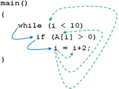
Blue (solid) lines represent control dependence. Green (broken) lines represent data dependence.
Figure 1: Dependence cluster example
form calledcoherentdependence clusters, followed by a review of the existing dependence cluster visualization techniques.
2.1
Dependence Clusters
Harman et al. [?] defined adependence clusteras a maximal set of program statements that mutually depend upon one another.
Definition 1 (Mutually-Dependent Cluster [?])
AMutually-Dependent Clusteris a maximal set of statements,S, such that∀x, y∈S:xdepends ony.
The above definition is parameterized by an underlying depends-onrelation. Ideally, such a relation would precisely represent the impact, influence, or dependence of one statement upon another. Unfortunately, such a relation is not computable. One well known approximation is based on Weiser’sProgram Slice[?]: a slice is a set of program statements that affect the values computed at a statement of interest. One common slicing algorithm is based on a program’s System Dependence Graph (SDG) [?]. An SDG is comprised of vertices, which essentially represent the statements of the program, and edges, which represent the immediate control and data dependence between vertices.
Two kinds of SDG slices are used in this paper: backward slices and forward slices. The backward slice taken with respect to vertex v, denotedBSlice(v), is the set of vertices reachingvvia a path of control and data dependence edges [?]. The second kind of slice, a forward slice, is also taken with respect to vertexv. Denoted FSlice(v), it includes the set of vertices reachable fromvvia a path of control and data dependence edges [?]. In both cases, when slicing programs that contain certain language features, the path of dependence edges considered must be restricted, for example, to respect the procedure calling convention of the language [?].
The following definitions are given usingBSlice. Each has a dual that usesFSlice. When the distinction is important,backward
andforwardwill be added to the definition name for clarification.
Definition 2 (Slice-based Cluster [?])
ASlice-based Clusteris a maximal set of vertices,V, such that ∀x, y∈V :x∈BSlice(y).
As a simple illustrative example of a slice-based dependence cluster, consider the example in Figure??. In this example, the predicatei<10data depends on the assignment toi, this assign-ment control depends on the predicate of theifstatement, and theif
control depends on the predicatei<10. As a result, all three state-ments are mutually inter-dependent (or in each other’sBSlice); they form a cluster.
Definition??for slice-based clusters permits clusters to over-lap. An alternative identifies maximal partitions. Such partitions correspond to statements which closely model the components that work together within a program. The partitioning can be achieved
(a) B-MSG (b) F-MSG
[image:2.612.113.233.55.145.2]y-axis: Slice Size (percent of program) x-axis: Slice Rank (percent of program)
Figure 2: MSGs for the programbc.
by replacing theslice inclusionrelationship of Definition??with
same-slice:
Definition 3 (Same-Slice Cluster [?])
ASame-Slice Clusteris a maximal set of vertices,V, such that ∀x, y∈V :BSlice(x) =BSlice(y).
Along with the internal requirement found in the slice inclusion definition of a Slice-based Cluster, a Same-Slice Cluster has the added external requirement that, all vertices in the cluster are af-fected by the same vertices external to the cluster. Coherent (depen-dence) clusters extend this external requirement to further include the external vertices affected by the elements of a cluster. The ex-tension has the advantage that the entire cluster is both affected by the same set of vertices (as is the case with same-backward-slice clusters) and also affects the same set of vertices (as is the case with same-forward-slice clusters). Incorporating internal depen-dence and both kinds of external dependepen-dence, Coherent Clusters are defined as follows:
Definition 4 (Coherent Cluster [?])
ACoherent Clusteris a maximal set of verticesV, such that ∀x, y∈V :xdepends onaimpliesydepends onaandadepends onximpliesadepends ony.
A slice-based instantiation for the above definition of coherent cluster isCoherent-Slice Cluster.
Definition 5 (Coherent-Slice Cluster [?])
ACoherent-Slice Clusteris a maximal set of vertices,V, such that
∀x, y∈V :BSlice(x) =BSlice(y)∧FSlice(x) =FSlice(y)
2.2
Cluster Visualizations with Size-Graphs
Three size-based graphs have been previously considered to vi-sualize dependence clusters: theMonotone Slice-Size Graph, theMonotone Cluster-Size Graph and the Slice/Cluster-Size Graph. First, as illustrated in Figure??, the Monotone Slice-Size Graph (MSG) [?] plots a landscape of monotonically increasing slice sizes where thex-axis includes each slice, in increasing order, and the y-axis shows the size of each slice as a percentage of the entire program. MSGs drawn using backward slice sizes are referred to as backward-slice MSG (B-MSG), those drawn using forward slice sizes are referred to as forward-slice MSG (F-MSG). In an MSG a dependence cluster appears as a sheer-drop cliff face followed by a plateau. For example, the B-MSG in Figure??a shows a large plateau depicting a same-backward-slice cluster spanning almost 70% of the programbc.
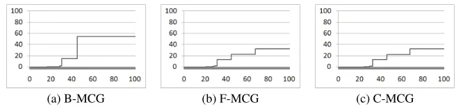
(a) B-MCG (b) F-MCG (c) C-MCG
[image:3.612.138.471.51.128.2]y-axis: Cluster Size (percent of program) x-axis: Cluster Rank (percent of program) Figure 3: MCGs for the programbc.
order with the sizes (as a percentage of the entire program) plot-ted on they-axis. MCGs can be drawn using the sizes of same-backward-slice clusters (B-MCG), same-forward-slice clusters (F-MCG), or coherent-slice clusters (C-MCG). In an MCG a pro-gram’s (same-slice/coherent-slice) clusters are clearly identified as steps. For example, MCGs in Figure??show the presence of two large same-backward-slice clusters, three same-forward-slice clus-ters and three coherent-slice clusclus-ters.
Finally, a combination of the MSG and MCG, the Slice/Cluster-Size Graph (SCG) [?] links slice and cluster sizes. As illustrated in Figure??an SCG plots three landscapes, one for increasing slice sizes (solid black line), one for the corresponding same-slice cluster sizes (light gray line), and the third for the corresponding coherent-slice cluster sizes (dashed red (gray in black & white) line). In the SCG, vertices are ordered along thex-axis first according to their slice size, second according to their same-slice cluster size, and third according to the coherent-slice cluster size. Three values are plotted on they-axis: slice sizes form the first landscape, while cluster sizes form the second and third. Two variants of the SCG are used: the backward-slice SCG (B-SCG) is built from the sizes of backward slices, same-backward-slice clusters, and coherent-slice clusters, while the forward-slice SCG (F-SCG) is built from the sizes of forward slices, same-forward-slice clusters, and coherent-slice clusters. SCGs ofbc(Figure??) show three coherent clusters along with the same-slice clusters. The backward and forward slice size for the vertices of the clusters are also shown, providing a link between clusters and the underlying slice sizes.
3.
IMPROVED VISUALIZATION
Building on previous visualizations that show only slice and clus-ter statistics, this section first presents design considerations for the new visualization. It then describes the proposed visualization’s four views of a program: the heat-map and three code-based views. Finally, the section ends with a discussion of the data acquisition process used to gather data from which the visualizations were gen-erated.
3.1
Design Consideration
Several guidelines have been proposed for the construction of ef-fective visualization tools. Two of these are used to ensure that de-cluviis of high-quality. First is the framework proposed by Maletic et al. [?] and second is the interface requirements proposed by Shneiderman [?]. Maletic et al.’s framework considers thewhy,
who, what, where, andhow of a visualization. Fordecluvithis leads to the following:
Tasks -why will the visualization help?
The visualization helps to quickly identify computations in-volved in clusters of dependence also shows interactions be-tween these computations. This identification makes it easier to understand and modify a program. The visualization also
(a) B-SCG (b) F-SCG
y-axis: Slice/Cluster Size (percent of program) x-axis: Slice/Cluster Rank (percent of program)
Figure 4: SCGs for the programbcwhere slice sizes are shown in solid black line, same-slice cluster sizes are shown in light gray line, and coherent-slice cluster sizes in dashed red (gray in black & white) line.
helps identify files and functions where multiple clusters are involved. Here re-structuring will improve cohesion and de-sign abstraction.
Audience -who will make use of the visualization?
Maintainers will use the visualization to gain overall under-standing of the program and estimate the impact of changes. Developers will also use the visualization to check if their implementation matches their documented architecture and to identify potential problems in the structure.
Target -what data source is to be represented?
Details of dependence clusters calculated from program. Medium -where to represent the visualization?
The visualization will involve highly interactive computer graphics being displayed on a color monitor.
Representation -how to represent the data?
The representation of the data will be through various ab-stract and concrete views (Sections??& ??), allowing both an overall architectural understanding of the system and also details of the implementation.
Shneiderman’s requirements are aimed at providing high-quality interfaces for visualization tools. They includeOverview, Zoom, Filter, Details-on-demand, Relate, HistoryandExtract. These fea-tures were used to guide the development ofdecluviand are pre-sented in Section??making it possible to evaluate the tool’s inter-face against these requirements.
3.2
Heat-Map View
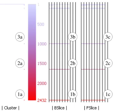
[image:3.612.317.557.173.260.2]loca-n
~ 1a
n
~ 2a
n
~ 3a
n
~ 1b
n
~ 2b
n
~ 3b
n
~ 1c
n
~ 2c
n
[image:4.612.78.270.51.240.2]~ 3c
Figure 5: Heat-Map View for the programbcshowing the color spectrum (shades of gray in black & white) used to represent cluster size.
tions on which to focus re-factoring efforts in order to improve the logical separation, cohesion, abstraction, and reduce code deterio-ration during evolution.
TheHeat-Map Viewis the central starting point to the visual-ization that displays an overview of all the clusters using color to distinguish clusters of varying sizes. The same color scheme is also used to represent the cluster size metric in other abstract and con-crete views. The view also displays additional statistics such as the size of the backward and forward slices for each coherent cluster and number of clusters for each cluster size. Figure??shows the Heat-Map View forbc, which has been annotated for the purpose of this discussion. The three labels1a,1b, and1chighlight statis-tics for the largest cluster (Cluster1) of the program, whereas2a,
2b, and2chighlight statistics of the2ndlargest cluster (Cluster2) and the3’s the3rd largest cluster (Cluster3). Starting from the left of the heat-map, using one pixel per cluster, horizontal lines (capped at 100 pixels) show the number of clusters that exist for each cluster size. This helps identify cases where there are multi-ple clusters of the same size. For exammulti-ple, the single dot next to the labels1a,2aand3ashow that there is one cluster of each of the three largest sizes. A single occurrence is common for large clus-ters, but not for small clusters as illustrated by the long line at the top left of the heat-map. This line indicates multiple (uninteresting) clusters having size one.
On the right of the cluster counts is the actual heat-map (color spectrum) showing dependence cluster sizes from small to large going from top to bottom using colors varying from blue to red. In gray-scale this appear as shades of gray, with lighter shades (corre-sponding to blue) representing smaller clusters and darker shades (corresponding to red) representing larger clusters. Red is used for larger clusters as they are more likely to encompasses complex functionality making them more important, or “hot topics”.
A numeric scale runs on the right of the heat-map, where the numbers show the cluster size (measured in SDG vertices) repre-sented by the color at the same horizontal level as the number. In Figure??, the scale forbcruns from 1 - 2432, depicting the sizes from the largest to the smallest clusters, displayed using bright red (dark gray) to light blue (light gray), respectively.
Finally on the right of the number scale, two more statistics are displayed:|BSlice|(labeled1b, 2band3b) and|FSlice|(labeled
1c, 2cand3c). These represent the sizes of the backward slice and
the forward slice for the vertices that form a coherent cluster. The sizes are shown as a percentage of the entire program’s SDG size (vertex count), with the separation of the vertical bars represent-ing 10% of the SDG size. For example, Cluster 1’sBSlice(1b) andFSlice(1c) include approximately 80% and 90% of the pro-gram’s SDG vertices. For this particular example, theFSlice’s and
BSlice’s that make up the top three clusters are very similar in size, resulting in bars of almost the same length.
3.3
Three Code-Based Views
The level of abstraction offered by a visualization must cope with the volume of code being visualized, which ranges from thousands of lines in a moderately sized system to millions of lines in a larger system. If a view is too detailed it becomes incomprehensible for the analysis of large systems. On the other hand, if the level of abstraction is too high, low-level detail is lost. In addition, pro-grammers are most comfortable in the spatial structure in which they have written the program. Therefore, a view of the source is often preferred. However, a single glance at a high-level view of the entire system allow engineers to ascertain the level of clustering and understand overall system structure. As a compromise between these conflicting needs, the visualization provides three different views that allow a program’s clusters to be viewed at varying levels of detail:System View,File View, andSource View.
The bird’s eye view shown by theSystem Viewis at the high-est level of abstraction. Each file of the system (containing exe-cutable source code) is abstracted into a column. This yields the nine columns forbc, seen in Figure??a. The name of the file ap-pears at the top of each column, color coded to reflect the largest cluster in the file. The vertical length of a column represents the length of the corresponding source file. To keep the view com-pact, each line of pixels in a column summarize multiple source lines. For moderate sized systems, such as the two case studies pre-sented, each pixel line typically represents eight source code lines. The color of each pixel line reflects the largest cluster found among the summarized lines of code, with light gray denoting source code lines that do not include executable code. Finally, the numbers at the bottom of each column indicate the presence of the top 10 clus-ters in the file (1 denotes the largest cluster of the program whereas 10 is the 10thlargest cluster).
Fig-(a)Unfiltered:Displaying all clusters using heat-map colors (b)Filtered:Displaying only Cluster 1 and 2 using heat-map colors Figure 6: System View for the Programbcshowing each file using one column, and each line of pixels summarizing cluster size data fromeightsource lines.
ure??b where only Cluster 1 is shown in red (dark gray), the rest of the cluster are filtered out (displayed in light gray). The filtering enables visual separation of a set of clusters (of interest), allowing one to easily examine the artifacts (lines/functions/files) that make up the clusters, and understand their interaction.
TheFile View, illustrated in Figure??, is at a lower level of ab-straction than the System View. It essentially zooms into a column of the System View. In this view, each pixel line corresponds to one line of source code. The pixel lines are also indented to mimic the indentation of the source lines and the number of pixels used to draw each pixel line is the same as the number of characters in the represented source code line. This makes it easier to relate this view to actual lines of source code. The color of the pixel line de-picts the size of the largest cluster to which any of the SDG vertices representing the corresponding source code line belong. Figure?? shows the Line View ofbc’s fileutil.c, filtered to show only the two largest clusters using colors of the heat-map, while smaller clusters and non-executable lines are shown in light gray. The lines shown in red (dark gray) and blue (medium gray) belong to Clusters 1 and 2, respectively.
While the first two views aid in locating parts of the system in-volved in one or more clusters, theSource Viewallows a program-mer to see the actual source code that makes up the cluster. This can be useful in addressing questions such as: Why are the clus-ters formed? What binds the cluster together? Is there dependence pollution? TheSource Viewillustrated in Figure??is a concrete view that maps the clusters onto actual source code lines. The lines are displayed in the same spatial context in which they were writ-ten, line color depicts the size of the largest cluster to which the SDG vertices representing the line belong. Figure??shows lines 241-257 ofbc’s fileutil.cwhich has also been filtered to show only the largest two clusters using colors from the heat-map. The lines of code whose corresponding SDG vertices are part of the largest cluster are shown in red (dark gray) and those lines whose SDG
vertices are part of the second largest cluster are shown in blue (medium gray). Other lines that do not include any executable code or whose SDG vertices are not part of the two largest cluster are shown in light gray. On the left of each line is aline tag, which denotes asa:b|c/d: the line number (a), the cluster number (b), and an identificationc/dfor thecthofdclusters having a given size. For example, in Figure?? lines 250 and 253 are both part of the20thlargest cluster (clusters with same size have the same rank) as indicated by the value ofb; however they belong to dif-ferent clusters as indicated by the differing values ofcin their line tags.
3.4
Data Acquisition
The visualization is generated from backward and forward slices taken with respect to each vertex of a program’s SDG. The slices along with the mapping between the SDG vertices and the actual source code is extracted from the mature and widely used slicing toolCodeSurfer[?]. The cluster sizes measured bydecluviis in terms of the SDG vertices; which exclude pseudo vertices intro-duced into the SDG, to represent, for example, global variables, which are modeled as additional pseudo parameters by CodeSurfer. Measuring size in terms of vertices is more accurate than using lines of code because it is not influenced by blank lines, comments, statements spanning multiple lines, multiple statements in one line, or compound statements.
4.
USE-CASE AND EVALUATION
This section presents a qualitative evaluation of coherent depen-dence clusters and their visualization. Two case-studies based on the programsbcand copiaare presented, followed by a discus-sion of threats to validity. The section ends with the evaluation of
decluvi’s user-interface.
Figure 7: File View (filtered) for the fileutil.cof Programbc. Each line of pixels correspond to one source code line. Blue color (medium gray in black & white) represents2nd largest cluster, and red color (dark gray) represents the largest clus-ter. The rectangle in the first column marks functioninit_gen
which contains both clusters.
This subsection presents a case study of the programbc. It starts with a brief description of the program followed by the results of applying the visualization to the program. The programbcis an open-source calculator, which consists of 16,763 LOC (lines of code as counted by the Unix utilitywc) and 11,173 SLoC (non-comment non-blank lines of code as counted bysloc[?]). The program has nine C files for which CodeSurfer produces 15,076 slices (backward and forward).
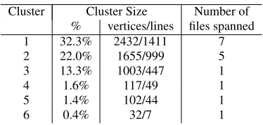
The Heat-Map View forbc(Figure??) shows the presence of three large clusters and three smaller clusters which are readily dis-tinguishable from each other. We will focus on these six clusters (detailed in Table??) as the rest of the clusters are extremely small: while the largest clusters consists of 2432 vertices, the7thlargest cluster consists of a mere 25 vertices.
As seen in Figure??, Cluster 1 spans all files inbcexcept for
scan.candbc.c. This cluster encompasses the core functionality of the program –loading and handling of equations, converting to bc’sown number format, performing calculations, and accumulat-ing results.
Cluster 2 spans five files,util.c, execute.c, main.c, scan.c,and
bc.c. The majority of the cluster is distributed over the last two
[image:6.612.56.282.50.403.2]Figure 8: Source View (filtered) showing functioninit_genin fileutil.cof Programbc. Blue color (medium gray in black & white) represents2ndlargest cluster and red color (dark gray) represents the largest cluster.
Figure 9: Source View for the filenumber.c of Program bc
showing the lines whose vertices form the6thlargest cluster.
Cluster Cluster Size Number of
% vertices/lines files spanned
1 32.3% 2432/1411 7
2 22.0% 1655/999 5
3 13.3% 1003/447 1
4 1.6% 117/49 1
5 1.4% 102/44 1
6 0.4% 32/7 1
Table 1: TopSixcoherent clusters ofbc
files. Even more interestingly, these two files contain only Cluster 2 from the set of the top 6 clusters, which indicates a clear purpose to the existence of the files. The files are solely used forlexical analysisandparsingof equations. To aid in this task some utility functions fromutil.care employed. Only five lines of code in ex-ecute.care part of Cluster 2 and are used forflushing outputand
clearing interrupt signals.
The third cluster is completely contained within the file num-ber.cand spans 1003 vertices. The cluster encompasses functions such as_bc_do_sub, bc_init_num, _bc_do_compare, _bc_do _add, _bc_simp_mul, _bc_shift_addsub,and_bc_rm _lead-ing_zeros, which are responsible forinitializingbc’snumber for-matter, performing comparisons, moduloand otherarithmetic op-erations. Clusters 4 and 5 are also completely contained within
number.c. These clusters encompass functions to performbcd op-erations for base ten numbersandarithmetic division, respectively. Cluster 6 (Figure??) ofbcspanning (32 vertices) 7 lines of code is formed because of awhile loopwhich checks if the exponent is zero.
[image:6.612.343.530.370.459.2]understand-(a)Original (b)Modified
Figure 10: SCGs for the programcopia
ing how the artifacts (functions/files) of the program interact to pro-vide various functionalities. The visualization thus aids in program comprehension. The following illustrates how the visualization can also aid in finding potential problems and its causes.
Util.cconsists of small utility functions called from various parts of the program. This file contains parts of Cluster 1 and 2. Both the separate functionalities identified previously (encompassed by each of the clusters) make use of the utility functions defined within the file. Figure??shows that two clusters in red (dark gray) and blue (medium gray) within the file are well separated. The clusters do not intersect inside any function with the exception ofinit_gen
(rectangle in first column of Figure??). The Code View of this function illustrated in Figure?? shows lines 244, 251, 254, and 255 in red (dark gray) from Cluster 1, and lines 247, 248, 249, and 256 in blue (medium gray) from Cluster 2. Other lines belonging to smaller clusters and those not containing any executable code are shown in light gray. Functions should be refactored to avoid containing more than one cluster as such functions reduce code separation (hindering comprehension) and increase the likelihood of ripple-effects [?]. A common exception to guidelines are initial-ization functions such asbc’sinit_gen, which initializes the parser code generator. The remaining functions belonging to each cluster should be separated by splittingutil.cinto two files, with each file dedicated to functions interacting with one of the two largest clus-ters. This would improve logic separation and cohesion at the file level, making the code easier to understand and maintain.
Frombc’s SCGs (Figure??) two interesting observations can be made. First, the programbccontains two large same-backward-slice clusters as opposed to three large same-forward-same-backward-slice clusters visible in the light gray landscapes. Secondly, looking at the B-SCG it can be seen that the space corresponding to the largest same-backward-slice cluster is occupied by two coherent-slice clusters shown in dashed red (dark gray) landscape. This indicates that the same-backward-slice cluster splits into the two coherent-slice clusters, supporting the conjecture that coherent clusters are more suited to modeling components of a program than other forms of dependence clusters.
The visualization reveals the high-level structure for the program
bcand shows how different artifacts (functions/files) of the pro-gram interact with each other. This makes it easier for engineers to understand the program. By identifying artifacts of the program which have multiple embedded functionalities, the visualization also identifies areas of low cohesion. These can be sources of code degradation during evolution. By highlighting such problems, the visualization successfully suggests artifacts that should be the focus of refactoring efforts. The slice/cluster sizes from the visualization provides an estimate of the level of difficulty likely to be faced by testers and maintainers when dealing with program. Artifacts that are part of larger clusters are harder to test and modify than those that are part of smaller clusters.
[image:7.612.53.294.52.134.2]4.2
Case Study
copia
Figure 11: File View for the filecopia.cof Programcopia. Each line of pixels represent the cluster size data for one source code line.
This subsection presents a case study ofcopia, an industrial pro-gram used for ESA signal processing. The propro-gram consists of 1,170 LOC, and 1,112 SLoC. It has only one C file from which CodeSurfer extracts 7518 slices (backward and forward). The pro-gramcopiahas a large coherent cluster spanning 40% of the B-SCG as shown by the dashed red (dark gray) line (running from 10% to 50% on thex-axis) in Figure??a.
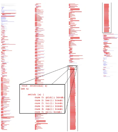
During the analysis ofcopia’s File View we were drawn towards an intriguing structure. There is a huge block of code with same spatial arrangement (bounded by black rectangle in Figure??) that belongs to a single large cluster of the program. It is unusual for so many consecutive source code lines to have similar length and in-dentation. Source View of the the corresponding lines revealed that this unusual large block of code is aswitchhandling 234 cases. Upon inspection ofcopiait was found that the program has 234 small functions that all call one large function,seleziona, which in turn calls the smaller functions effectively implementing a finite state machine. Each of the smaller functions return a value that is the next state for the machine and is used by the switch to call the appropriate function. The primary reason for the high level of de-pendence in the program lies in the statementswitch(next_state), which controls the call to the smaller functions. This causes what might be termed ‘conservative dependence analysis collateral dam-age’ because the static analysis can not determine that when func-tionf()returns a 5 this causes the switch statement to eventually invoke functiong(). Instead, the analysis makes the conservative assumption that a call tof()might be followed by a call to any of the functions appearing in the switch statement, resulting in a mu-tual recursion involving most of the program.
Figure 12:decluvi’s Control Panel showing buttons to toggle views, configure filter range, and hide filtered regions.
statement. The SCGs for bothoriginalandmodified versions of the program are shown in Figure??. As seen in the figure, remov-ing the switch and its control dependence removes the cluster. As a result of this reduction, the potential impact of changes to the pro-gram will be greatly reduced, making it easier to understand and maintain.
In this particular case study, owing to peculiar coding structure, the visualization was used to identify the cause of the cluster. This however is not the primary purpose of the visualization. The visu-alization as presented can show the existence of clusters, helping in program comprehension, but cannot pinpoint a cause of the clus-ters. It currently can only assist in investigating the program for possible causes. However, it is not difficult to incorporate other techniques [?,?] of identifying causes of dependence clusters and view them using the presented visualization.
Finally, in the B-SCG forcopia(Figure??a) it is seen that the plots for Backward-Slice Cluster Sizes (light gray line) and the co-herent cluster sizes (dashed red (gray in black & white) line) are very similar. This has happened because, in this case the size of the coherent-slice clusters are restricted by the size of the same-backward-slice clusters. Although, the plot for the size of the back-ward slices (black line) seems to be the same from the 10% mark to 95% mark on thex-axis, the slices are not exactly same size. Only vertices plotted from 10% through to 50% have exactly same backward slice. The tolerance implicit in the visual resolution used to plot the slice sizes obscures this detail.
The case study forcopiashows that the visualization can not only show the existence and distribution of coherent clusters, but the detailed views can also lead to identification of dependence pollution. Restructuring of such programs to remove the pollution, makes the program easier to understand, test and maintain.
4.3
Threats to Validity
In the study, the primary threat arises from the possibility that the selected programs are not representative of programs in general (i.e., the findings of the experiments do not apply to ‘typical’ pro-grams). This is a reasonable concern as we present only two case studies. The programs presented are however from different do-mains: one open-source and another industrial, both of which have previously been the subject of many studies. Also, the programs studied to date, including the two case studies, are mid-sized. It is possible that the value of the visualization does not scale to larger systems. Finally, a threat arises from the potential for faults in the slicer. A mature and widely used slicing tool (CodeSurfer) was used to mitigate this concern.
4.4
decluvi’s Interface Evaluation
This subsection provides an evaluation ofdecluvi’s user interface against the list of features suggested by Shneiderman [?].
Overview -Gain an overview of the entire collection of data that is represented.
The abstract Heat-Map View and compact System View pro-vide an overview of the clustering for an entire system. Zoom -Zoom in on items of interest.
From the System View it is possible to zoom into individual files in either a lower level of abstraction (File View) or the concrete (Source View) form.
Filter -Filter out uninteresting items.
The control panel, shown in Figure??, includes sliders and ‘fast cluster selection’ buttons. These allow a user to filter out uninteresting clusters and thus focus only on clusters of interest. The tool also provides option to hide non-executable lines and clusters whose size fall outside a specified range. Details-on-demand: -Select an item or group and obtain details
when needed.
Although details for all items shown in the visualization can-not be obtained, cluster related details are available. For ex-ample, clicking on a column of the System View opens the File View for the corresponding file and clicking on a line in the File View highlights the corresponding line in the Source View. Finally, the fast cluster selection buttons allow the user to demand and get details on a given cluster.
Relate -Clear relationship between the various views.
There is a hierarchical relationship between the various views provided bydecluvi. Common coloring is used throughout to tie abstract elements of the higher level views with the con-crete source lines in the Source View. In addition, File View and Source View preserve the layout of the underlying source code (e.g., the indentation of the lines).
History -Keep history of actions to support undo, replay and pro-gressive refinement.
Decluvicurrently meets this requirement partially. The var-ious views of the tool retain their settings and viewing po-sitions when toggled. However, current version ofdecluvi
lacks support for undo, replay, or history.
Extract -Allow extraction of sub-collections and of the query pa-rameters.
The tool provides support for exporting slice/cluster statis-tics.
5.
RELATED WORK
The work presented follows two separate sub-domains of soft-ware engineering. The first is dependence cluster analysis and the second is software visualization. The following subsections de-scribe relevant work from these sub-domains.
5.1
Dependence Clusters
Binkley and Harman [?] were the first to introduce the notion of dependence clusters that looked into the fine grained structure of clustering based on vertices of an SDG. They deemed depen-dence clusters as problems for software maintenance and regarded them as anti-patterns [?], pollution [?] and bad code smells [?]. Black [?] has even hypothesized a direct relationship between the size of dependence clusters and number of software faults. Bink-ley et al. followed up their initial work and presented work on the causes (low-level [?] and high-level [?]) of dependence clusters. Islam et al. [?] have recently introduced coherent clusters suggest-ing that such clusters have the potential to reveal high-level struc-tures of systems.
5.2
Software Visualization
Binkley et al. [?] were the first to introduce a graph visualiza-tion for dependence clusters known as MSG. Islam et al. [?] later extended this by introducing MCG and SCG. All these three visu-alizations were however size-graphs aimed solely at showing the presence of dependence clusters and their statistics. These visual-izations do not aid in program understanding as they lack a map-ping to source code.
SeesoftSystem [?] is a seminal tool for visualizing line oriented software statistics. The system pioneered the idea of abstracting source code view to represent each source code line using a line of pixels. This allowed for visualization of up to 50,000 lines of code on a single screen. The rows were colored to represent the values of statistics being visualized. The system pioneered four key ideas: reduced representation, coloring by statistic, direct manipulation, and capability to read actual code. The reduced representation was achieved by displaying files as columns and lines of code as thin rows. The system was originally envisioned to help in a lot of areas including program understanding. Ball and Eick [?] also presented
SeeSlice, a tool for interactive slicing. This was the first slicing vi-sualization system that allowed for a global overview of a program. Our visualization inherits these approaches and extends them to be effective for dependence clusters.
The approach pioneered bySeesoftwas also used in many other visualization tools. SeeSys System [?] was developed to local-ize error-prone code through visualization of ‘bug fix’ statistics. The tool extended the Seesoft approach by introducing treemaps to show hierarchical data. It displayed code organized hierarchically into subsystems, directories, and files by representing the whole system as a rectangle and recursively representing the various sub-units with interior rectangles. The area of each rectangle was used to reflect statistic associated with its sub-unit. Tarantula [?] also employs the “line of pixel” style code view introduced by Seesoft. The tool was aimed at visualizing the pass/fail of test cases. It ex-tended the idea of using solid colors to represent statistics by using hue and brightness to encode additional information. CVSscan [?] also inherited and extended the “line of pixel” based representa-tion by introducing “dense pixel display” to show the overall evo-lution of programs. The tool has a bi-level code display that pro-vide views of both the contents of a code fragment and its evolution over time. Source Viewer 3D [?] is a software visualization frame-work that is based on Seesoft and adds a third dimension (3D) to the original approach allowing additional statistics to be visualized. Augur [?] is also based on the line-oriented approach of Seesoft. The primary view is spatially organized as in Seesoft with addi-tional columns to display multiple statistics for each line. Aspect Browser (Nebulous) [?] provides a global view of how the various aspect entries cross-cut the source code using “line of pixels” view and uses Aspect Emacs to get the statistics and provide the concrete source code view. BLOOM [?] uses the BEE/HIVE [?] architec-ture, a powerful back-end that supports a variety of high-density, high-quality visualization one of which (File Maps) is based on the Seesoft layout.
The final set of systems discussed are those that aim to help in reverse engineering but are not based on the “line of pixels” ap-proach. Most of these tools focus on visualizing high-level system abstractions (often referred to as ‘clustering’ or ‘aggregation’) such as classes, modules, and packages, using a graph-based approach. Rigi [?] is a reverse engineering tool that uses Simple Hierarchi-cal Perspective (SHriMP) views, employs fisheye views of nested graphs. Creole [?] is an open-source plugin for the Eclipse (IDE) based on SHriMP. Tools such as GOOSE [?], Sotograph [?] and VizzAnalyzer [?] work on the class and method levels allowing in-formation aggregation to form higher levels of abstractions. There
are tools (Borland Together, Rational Rose, ESS-Model, BlueJ, Fu-jaba, GoVisual [?]) which also help in reverse engineering by pro-ducing UML diagrams from source code.
6.
FUTURE WORK
Future work will involve a wide-scale qualitative study into how well decluvisupports software comprehension and maintenance. The feedback and survey results form such work can be used to further improvedecluvi. Preliminary evidence for the success of such study is found in the case studies ofbcandcopiawhere we identified several improvements that will makedecluvimore effec-tive:
• Addition of intermediate abstractions to visualize clusters at function, component and directory level. This will make it easier to understand the inter-play of clusters and help focus on re-engineering of artifacts containing multiple clusters. • Improve the algorithm used to calculate color for the pixel
lines in the System View by adding anti-aliasing features to incorporate cluster size statistics from all summarized lines of source code.
• Add 3D to visualize the number of clusters of each size to address cases where multiple clusters have the same size and cannot be readily distinguished using color.
• Add support forhistory,undo, andreplayto allow users to backtrack their steps.
7.
CONCLUSION
The paper introduced new multi-level dependence cluster visu-alization that aids in comprehension, maintenance, and reverse en-gineering tasks. The visualization is realized usingdecluvi, which allows dependence clusters to be viewed in terms of source code rather than statistics. The two case studies show that the new visu-alization is able to reveal high-level structure of programs and can also be used to ascertain interaction between the different compo-nents of a program. The case study forbcillustrates that the visual-ization identifies artifacts with low cohesion where refactoring will make the code easier to understand and also reduce code deterio-ration during software evolution. The visualization also highlights dependence pollution and its causes incopiathat can hinder testing and maintenance.
Thedecluvisystem along with scheme script for data acquisition and pre-compiled dataset for several open-source programs can be downloaded from:
http://www.dcs.kcl.ac.uk/pg/syed/tools.html
8.
ACKNOWLEDGMENTS
We would like to thank GrammaTech Inc. (http://www. gramm atech.com) for making CodeSurfer available.
9.
REFERENCES
[1] Chisel Group. Creole Homepage:
http://www.thechiselgroup.org/creole. [2] GOOSE Homepage:http://esche.fzi.de/
PROSTextern/software/goose/index.html. [3] Software-Tomography GmbH. Sotograph Homepage:
http://www.software-tomography.com/html/ sotograph.htm.
[5] M. J. Baker and S. G. Eick. Space-filling software visualization.Journal of Visual Languages & Computing, 6(2):119 – 133, 1995.
[6] T. Ball and S. Eick. Visualizing program slices.Proceedings of 1994 IEEE Symposium on Visual Languages, pages 288–295, 1994.
[7] D. Binkley. Semantics guided regression test cost reduction.
IEEE Transactions on Software Engineering, 23:498–516, 1997.
[8] D. Binkley. Source code analysis: A road map.ICSE 2007 Special Track on the Future of Software Engineering, May 2007.
[9] D. Binkley, N. Gold, M. Harman, Z. Li, K. Mahdavi, and J. Wegener. Dependence anti patterns. In23rd IEEE/ACM International Conference on Automated Software Engineering, pages 25–34, September 2008.
[10] D. Binkley and M. Harman. Locating dependence clusters and dependence pollution. In21st IEEE International Conference on Software Maintenance, pages 177–186, 2005. [11] D. Binkley and M. Harman. Identifying ‘linchpin vertices’
that cause large dependence clusters. InNinth IEEE International Working Conference on Source Code Analysis and Manipulation, pages 89–98, 2009.
[12] D. Binkley, M. Harman, Y. Hassoun, S. Islam, and Z. Li. Assessing the impact of global variables on program dependence and dependence clusters.Journal of Systems and Software, April 2009.
[13] S. Black. Computing ripple effect for software maintenance.
Journal of Software Maintenance and Evolution: Research and Practice, 13:263–279, July 2001.
[14] S. Black, S. Counsell, T. Hall, and P. Wernick. Using program slicing to identify faults in software. InBeyond Program Slicing, number 05451 in Dagstuhl Seminar Proceedings, Dagstuhl, Germany, 2006.
[15] G. Canfora. An integrated environment for reuse reengineering C code.Journal of Systems and Software, 42:153–164, August 1998.
[16] S. Diehl. Software visualization. InICSE ’05: Proceedings of the 27th International Conference on Software Engineering, pages 718–719, New York, NY, USA, 2005. ACM. [17] S. Eick, J. Steffen, and E. Sumner. Seesoft-a tool for
visualizing line oriented software statistics.IEEE Transactions on Software Engineering, 18:957–968, 1992. [18] A. Elssamadisy and G. Schalliol. Recognizing and
responding to "bad smells" in extreme programming. In
International Conference on Software Engineering, pages 617–622, 2002.
[19] J. Froehlich and P. Dourish. Unifying artifacts and activities in a visual tool for distributed software development teams. InICSE ’04: Proceedings of the 26th International Conference on Software Engineering, pages 387–396, Washington, DC, USA, 2004. IEEE Computer Society. [20] K. B. Gallagher and J. R. Lyle. Using program slicing in
software maintenance.IEEE Transactions on Software Engineering, 17:751–761, 1991.
[21] M. Harman, K. Gallagher, D. Binkley, N. Gold, and J. Krinke. Dependence clusters in source code.ACM Transactions on Programming Languages and Systems, 32(1):1–33, 2009.
[22] S. Horwitz, T. Reps, and D. Binkley. Interprocedural slicing using dependence graphs.ACM Transactions on
Programming Languages and Systems, 12:26–60, January 1990.
[23] S. Islam, J. Krinke, D. Binkley, and M. Harman. Coherent dependence clusters. InPASTE ’10: Proceedings of the 9th ACM SIGPLAN-SIGSOFT Workshop on Program Analysis for Software Tools and Engineering, New York, NY, USA, 2010. ACM.
[24] J. A. Jones, M. J. Harrold, and J. T. Stasko. Visualization for fault localization. InProceedings of the Workshop on Software Visualization, 23rd International Conference on Software Engineering, May 2001.
[25] J. I. Maletic, A. Marcus, and M. L. Collard. A task oriented view of software visualization. InVISSOFT ’02:
Proceedings of the 1st International Workshop on Visualizing Software for Understanding and Analysis, page 32,
Washington, DC, USA, 2002. IEEE Computer Society. [26] A. Marcus, L. Feng, and J. I. Maletic. 3D representations for
software visualization. InSoftVis ’03: Proceedings of the 2003 ACM Symposium on Software Visualization, New York, NY, USA, 2003. ACM.
[27] K. J. Ottenstein and L. M. Ottenstein. The program dependence graph in software development environments.
Proceedings of the ACM SIGSOFT/SIGPLAN Software Engineering Symposium on Practical Software Development Environments, SIGPLAN Notices, 19(5):177–184, 1984. [28] T. Panas, J. Lundberg, and W. Lowe. Reuse in reverse
engineering. InIWPC ’04: Proceedings of the 12th IEEE International Workshop on Program Comprehension, page 52, Washington, DC, USA, 2004. IEEE Computer Society.
[29] S. P. Reiss. Bee/Hive: A software visualization back end.
Proceedings of ICSE 2001 Workshop on Software Visualization, Toronto, pages 44–48, 2001.
[30] S. P. Reiss. An overview of BLOOM. InPASTE ’01: Proceedings of the 2001 ACM SIGPLAN-SIGSOFT Workshop on Program Analysis for Software Tools and Engineering, pages 2–5, New York, NY, USA, 2001. ACM. [31] B. Shneiderman. The eyes have it: A task by data type
taxonomy for information visualizations. InVL ’96: Proceedings of the 1996 IEEE Symposium on Visual Languages, page 336, Washington, DC, USA, 1996. IEEE Computer Society.
[32] M.-A. D. Storey, K. Wong, and H. A. Müller. Rigi: a visualization environment for reverse engineering. InICSE ’97: Proceedings of the 19th International Conference on Software Engineering, pages 606–607, New York, NY, USA, 1997. ACM.
[33] L. Voinea, A. Telea, and J. J. van Wijk. CVSscan:
visualization of code evolution. InSoftVis ’05: Proceedings of the 2005 ACM Symposium on Software Visualization, pages 47–56, New York, NY, USA, 2005. ACM. [34] M. Weiser and C. Park. Program slicing. InInternational
Conference on Software Engineering, 1981. [35] D. A. Wheeler. SLOC count user’s guide.
http://www.dwheeler.com/sloccount/sloccount.html., 2004. [36] W. G. Yoshikiyo, W. G. Griswold, Y. K. Y, and J. J. Yuan.