Optimization of Roughness Value by using Tool Inserts of Nose Radius 1 2mm in Finish Hard Turning of AISI 52100 Steel

Optimization of Roughness Value by using Tool Inserts of Nose Radius

1.2mm in Finish Hard-Turning of AISI 52100 Steel

Mr. Vivekanand S. Swami

_{Mr. Pratik P. Mohite}

_{Prof. Pravin A. Dhavale}

_{Prof. Hemant G.}

Waikar

1,2

_{M.E. Student}

_{Associate Professor}

_{Assistant Professor}

1,2,3,4

_{Fabtech Technical Campus, Sangola, India}

Abstract— Increasing the productivity and the quality of the machined parts are the main challenges of high strength and heat resistant materials in aerospace, automotive, steam turbines and nuclear applications. This requires better management of the machining system corresponding to cutting tool-machine tool- study piece combination to go towards more rapid metal removal rate. In this work, a L9 Taguchi standard orthogonal array is adopted as the experimental design. The combined effects of the cutting parameters on roughness value are investigated. The relationship between cutting parameters and roughness values through the regression analysis is found out. The different correlations are developed between tribological parameters and roughness value for 0.4 mm of tool nose radius with 9 runs.

Key words: L9 Taguchi, Roughness Value, Cutting Parameters, Regression Analysis, Tribological Parameters

I. INTRODUCTION

Hard machining means machining of parts whose hardness is more than 45 HRC. Hard turning is a process which eliminates the requirements of grinding operation. A proper hard turning process gives surface finish Ra 0.4 to 0.8 μm, roundness about 2–5 μm and diameter tolerance ± 3–7 μm. Hard turning of highly hardened parts is a new approach in machining science aimed at increasing productivity and yield through reducing production time and costs of the process. This method has been introduced as a suitable alternative to grinding of hardened parts. Some decisive factors leading to this manufacturing trend are: substantial reduction of manufacturing costs, decrease of production time, achievement of comparable surface finish and reduction or elimination of environmentally harmful cooling media. The quality of surfaces of machined components is determined by the surface finish tester and integrity obtained after machining. High surface roughness values, hence poor surface finish, decrease the fatigue life of machined components.

In turning, there are many factors affecting the cutting process behavior such as tool variables, work piece variables and cutting conditions. Tool variables consist of tool material, cutting edge geometry (clearance angle, cutting edge inclination angle, nose radius, and rake angle), tool vibration, etc., while work piece variables comprise material, mechanical properties (hardness), chemicals and physicals properties, etc. Furthermore, cutting conditions include cutting speed, feed rate and depth of cut. The selection of optimal process parameters is usually a difficult work, however, is a very important issue for the machining process control in order to achieve improved product quality, high productivity and low cost. The optimization techniques of machining parameters through experimental methods and

mathematical and statistical models have grown substantially over time to achieve a common goal of improving higher machining process efficiency.

The turning operation is performed with tool materials mixed ceramic (Al2O3 + TiC) and cubic boron nitride (CBN), which induces a significant benefit, such as short-cutting time, process flexibility, low surface roughness of piece, high rate of material removal and dimensional accuracy.

The main challenge in hard turning is whether coolant will be used or not. In maximum cases hard turning is performed dry. When hard turning is performed without coolant, part is hot, which causes a difficulty in process gauging. To cool down the machined part coolant is used through the tool with high pressure. In hard turning maximum heat is transferred to chip so if chip is examined during and after cut, the process is said to be well turned if the chips is glowing orange and flow like ribbon during continuous cut. The potential benefits promoted by hard turning for surface quality and to increase the rate of productivity depend intrinsically an optimal setting for the process parameters such as cutting speed, feed rate and cutting depth.

II. PRESENT THEORIES & PRACTICES

Many researchers have worked on hard turning of metals with the help of single point inserts. Some of the notable works relevant to our study are summarized below:

K.Bouacha et.al. [1] carried out an experimental study of hard turning with CBN tool of AISI 52100 bearing steel, hardened at 64 HRC. The relationship between cutting parameters (cutting speed, feed rate and depth of cut) and machining output variables (surface roughness, cutting forces) through the response surface methodology are analysed and modeled. The combined effects of the cutting parameters on machining output variables are investigated while employing the analysis of variance (ANOVA). Results show how much surface roughness is mainly influenced by feed rate and cutting speed. Also, it is underlined that the thrust force is the highest of cutting force components, and it is highly sensitive to workpiece hardness, negative rake angle and tool wear evolution. Finally, the depth of cut exhibits maximum influence on cutting forces as compared to the feed rate and cutting speed.

A.Bagawade et.al. [2] expressed machinability of AISI 52100 hardened steel in terms of the performance variables such as MRR, cutting forces, tool wear, surface finish and surface integrity etc. In this investigation statistical analysis of the process was performed to explore the effect of the input factors on output variables.

uncoated CBN tool and to analyze the combination of the machining parameters for better performance within a selected range of machining parameters. A full factorial design of experiments procedure was used to develop the force and surface roughness regression models, within the range of parameters selected. The regression models developed show that the dependence of the cutting forces i.e. cutting, radial and axial forces and surface roughness on machining parameters are significant

A.Attanasio, et.al. [4]. studied the effects of tool wear and cutting parameters (cutting speed and feed rate), on white and dark layer formation in hardened AISI 52100 bearing steel, using PCBN inserts. Experimental results were presented including quantification of tool wear and microstructure analysis of the machined surfaces. The experimental results were compared with a newly developed finite elements model that enables to capture the effect of cutting conditions and tool wear on the microstructural changes occurring at the machined surface. The results showed that cutting regime parameters and, especially, tool wear affect noticeably white and dark layers formation.

S.Hosseini et.al. [5]. observed that hard turned surfaces can consist of a “white” and a “dark” etching layer having other mechanical properties compared to the bulk material depending on the process parameters and the tool condition . X-ray diffraction measurements revealed that tensile residual stresses accompanied with higher volume fraction of retained austenite are present in the thermally induced white layer. While compressive residual stresses and decreased retained austenite content was found in the plastically created white layer. The surface temperature was estimated to be 12000C during white layer formation by hard turning.

A. Agrawal et. al. [6] has studied in their article, Prediction of surface roughness during hard turning of AISI 4340. In his study, 39 sets of hard turning experimental trials were performed on a AISI 4340 material hardened up to 60 HRC to study the effect of cutting parameters in influencing the machined surface roughness. The machining outcome was used as an input to develop various regression models to predict the average machined surface roughness on this material. Three regression models – Multiple regression, random forest, and quantile regression were applied to the

experimental outcomes and a generalized mathematical equation was formed.

Paulo H.S.Campos et. al. [7] has stated in their published paper about Modeling Life of Tool and Roughness in Turning Hard Steel AISI 52100. They have studied the interrelationship between the life of tools, average roughness of the machined surfaces and the process factors such as cutting speed, feed, depth of cut in a single context. They have applied a statistical approach to derive a mathematical relationship between the influencing factors and a mathematical modeling tool life (T) and surface roughness (Ra, Rq) of the part in the process of turning of hardened steel. N. Gore et. al. [8] has studied the Optimization of Roughness Value from Tribological Parameters in Hard Turning of AISI 52100 Steel. The experimentation was performed on CNC machine and the CBN insert was used to optimize the roughness value of AISI 52100 steel which has hardness between 41 to 65 HRC under the tribological parameters like speed, feed and the depth of cut. The Taguchi L9 (OA) was utilized and the performance of roughness value was optimized by the regression analysis.

III. SCOPE OF WORK

In this work, an attempt will be made to investigate the effect of cutting parameters (cutting speed, feed rate and depth of cut) on the performance characteristics surface roughness in hard turning of hardened steel with hardness in between 41 to 68 HRC with CBN tool. In this work, a Taguchi standard orthogonal array is adopted as the experimental design. The combined effects of the cutting parameters on roughness values are investigated. The relationship between cutting parameters and roughness values through the regression analysis, the different correlations are developed between tribological parameters and roughness value.

IV. TAGUCHI DESIGN

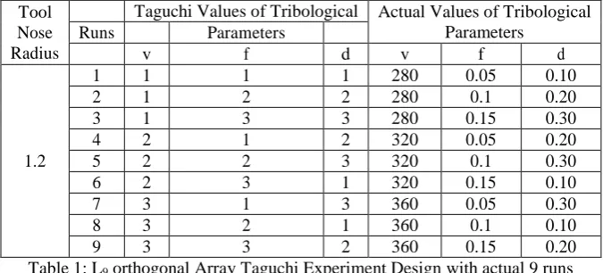
The working ranges of the parameters for subsequent design of experiment, based on Taguchi’s L9 (32_{) orthogonal array} (OA) design has been selected. In the present experimental work, cutting speed (v),feed rate (f),and depth of cut (d) have been consider as a cutting parameters. The cutting parameters and their associated ranges are given in the table below:

Tool Nose Radius

Taguchi Values of Tribological Actual Values of Tribological Parameters

Runs Parameters

v f d v f d

1.2

1 1 1 1 280 0.05 0.10

2 1 2 2 280 0.1 0.20

3 1 3 3 280 0.15 0.30

4 2 1 2 320 0.05 0.20

5 2 2 3 320 0.1 0.30

6 2 3 1 320 0.15 0.10

7 3 1 3 360 0.05 0.30

8 3 2 1 360 0.1 0.10

9 3 3 2 360 0.15 0.20

Table 1: L9 orthogonal Array Taguchi Experiment Design with actual 9 runs After that stepwise procedure is adopted for turning

operation and Mitutoyo make roughness tester is used for

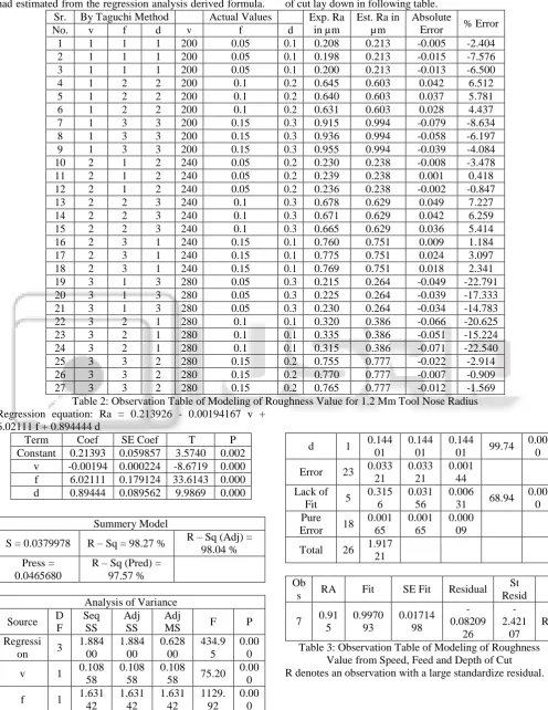
5] Modeling of roughness value from speed, feed and depth of cut for 0.4 mm tool nose radius: New value of roughness had estimated from the regression analysis derived formula.

At last the absolute error and the percentage error calculated. The modeling of roughness value from speed, feed and depth of cut lay down in following table.

Sr. By Taguchi Method Actual Values Exp. Ra

in µm

Est. Ra in µm

Absolute

Error % Error

No. v f d v f d

1 1 1 1 200 0.05 0.1 0.208 0.213 -0.005 -2.404

2 1 1 1 200 0.05 0.1 0.198 0.213 -0.015 -7.576

3 1 1 1 200 0.05 0.1 0.200 0.213 -0.013 -6.500

4 1 2 2 200 0.1 0.2 0.645 0.603 0.042 6.512

5 1 2 2 200 0.1 0.2 0.640 0.603 0.037 5.781

6 1 2 2 200 0.1 0.2 0.631 0.603 0.028 4.437

7 1 3 3 200 0.15 0.3 0.915 0.994 -0.079 -8.634

8 1 3 3 200 0.15 0.3 0.936 0.994 -0.058 -6.197

9 1 3 3 200 0.15 0.3 0.955 0.994 -0.039 -4.084

10 2 1 2 240 0.05 0.2 0.230 0.238 -0.008 -3.478

11 2 1 2 240 0.05 0.2 0.239 0.238 0.001 0.418

12 2 1 2 240 0.05 0.2 0.236 0.238 -0.002 -0.847

13 2 2 3 240 0.1 0.3 0.678 0.629 0.049 7.227

14 2 2 3 240 0.1 0.3 0.671 0.629 0.042 6.259

15 2 2 3 240 0.1 0.3 0.665 0.629 0.036 5.414

16 2 3 1 240 0.15 0.1 0.760 0.751 0.009 1.184

17 2 3 1 240 0.15 0.1 0.775 0.751 0.024 3.097

18 2 3 1 240 0.15 0.1 0.769 0.751 0.018 2.341

19 3 1 3 280 0.05 0.3 0.215 0.264 -0.049 -22.791

20 3 1 3 280 0.05 0.3 0.225 0.264 -0.039 -17.333

21 3 1 3 280 0.05 0.3 0.230 0.264 -0.034 -14.783

22 3 2 1 280 0.1 0.1 0.320 0.386 -0.066 -20.625

23 3 2 1 280 0.1 0.1 0.335 0.386 -0.051 -15.224

24 3 2 1 280 0.1 0.1 0.315 0.386 -0.071 -22.540

25 3 3 2 280 0.15 0.2 0.755 0.777 -0.022 -2.914

26 3 3 2 280 0.15 0.2 0.770 0.777 -0.007 -0.909

27 3 3 2 280 0.15 0.2 0.765 0.777 -0.012 -1.569

Table 2: Observation Table of Modeling of Roughness Value for 1.2 Mm Tool Nose Radius Regression equation: Ra = 0.213926 - 0.00194167 v +

6.02111 f + 0.894444 d

Term Coef SE Coef T P

Constant 0.21393 0.059857 3.5740 0.002 v -0.00194 0.000224 -8.6719 0.000

f 6.02111 0.179124 33.6143 0.000

d 0.89444 0.089562 9.9869 0.000

Summery Model

S = 0.0379978 R – Sq = 98.27 % R – Sq (Adj) = 98.04 % Press =

0.0465680

R – Sq (Pred) = 97.57 %

Analysis of Variance

Source D

F Seq SS Adj SS Adj

MS F P

Regressi

on 3

1.884 00 1.884 00 0.628 00 434.9 5 0.00 0

v 1 0.108

58

0.108 58

0.108

58 75.20

0.00 0

f 1 1.631

42 1.631 42 1.631 42 1129. 92 0.00 0

d 1 0.144

01

0.144 01

0.144

01 99.74

0.00 0

Error 23 0.033

21 0.033 21 0.001 44 Lack of

Fit 5

0.315 6

0.031 56

0.006

31 68.94

0.00 0 Pure

Error 18 0.001 65 0.001 65 0.000 09

Total 26 1.917

21

Ob

s RA Fit SE Fit Residual

St Resid

7 0.91

5 0.9970 93 0.01714 98 -0.08209 26 -2.421 07 R

V. EXPERIMENTAL & ESTIMATED ROUGHNESS VALUE FROM SPEED, FEED,& DEPTH OF CUT FOR DIFFERENT TOOL NOSE

RADIUS 1.2MM

The correlations developed from the statistical analyses, which are given below:

The below given equations are individual correlations with roughness value,

Ra = 0.994926 - 0.00194167 v …. (Eq. 1) Ra = -0.0731852 + 6.02111 f …. (Eq. 2) Ra = 0.350037 + 0.894444 d …. (Eq. 3) The below given equations are combined correlation with roughness value,

Ra = 0.392815 - 0.00194167 v + 6.02111 f …. (Eq. 4) Ra = 0.816037 - 0.00194167 v + 0.894444 d …(Eq. 5) Ra = -0.252074 + 6.02111 f + 0.894444 d …. (Eq. 6) The final equations have the all parameters effect on roughness value, Ra = 0.213926 - 0.00194167 v + 6.02111 f + 0.894444 d …. (Eq. 7)

The below given graphical representation show the correlation between estimated roughness value and experimental roughness value. The experimental roughness value is the actual roughness value measured by roughness tester and the estimated roughness are the values, which are estimated from regression equation and main factors cutting speed, feed, and depth of cut for 1.2mm tool nose radius.

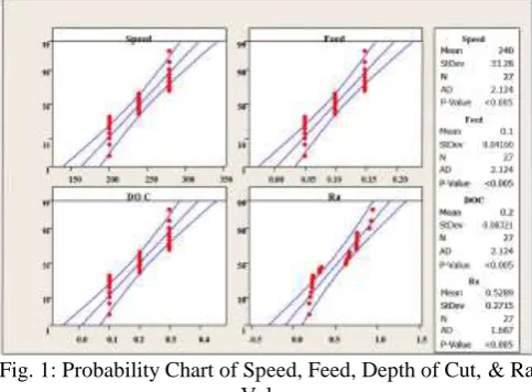
Graph 1: Number of Runs versus Experimental and Estimated Ra from Speed, Feed, and Depth of Cut The below given graph which shows the probability of speed, feed, depth of cut, and roughness value. For speed the mean value is 240 and the standard deviation is 33.28. Total 27 runs or the reading taken for the speed in calculations and the AD value is 2.124 which give the probability less than by the 0.005.

For feed the mean value is 0.1 and the standard deviation is 0.04160. Total 27 runs or the reading taken for the feed in calculations and the AD value is 2.124 which give the probability less than by the 0.005.

For depth of cut the mean value is 0.2 and the standard deviation is 0.08321. Total 27 runs or the reading taken for the depth of cut in calculations and the AD value is 2.124 which give the probability less than by the 0.005.

For the roughness value the mean value is 0.5289 and the standard deviation is 0.2715. Total 27 runs or the reading taken for the roughness value in calculations and the AD value is 1.687 which gives the probability less than by the

At last the probability values by Anderson – Darling test’s (AD test’s) for speed, feed, depth of cut, and roughness value are the 0.005, which are less than by 0.05 (5% level of significance) which indicates that the data do not follow the normal distribution. So it fails to accept the null hypothesis.

Fig. 1: Probability Chart of Speed, Feed, Depth of Cut, & Ra Value

VI. CONCLUSIONS

The conclusions drawn from the analysis are given below:  In hard turning, the taguchi method has proved to be

efficient tools for controlling the effect tribological parameters on roughness value.

 The speed, feed, and depth of cut plays equally important role in the machining process but in analysis the feed and depth of cut showed an excellent bonding effect on roughness value prediction form the regression analysis. The speed has shown less effect on roughness value.  As the number of tribological parameters increases in the

co relational analysis the correlation value increases simultaneously.

 For single tribological parameters the equation would be able to predict the roughness value with accuracy from (R2 _{value) 5.66 to 85.09 % and for combine tribological} parameters the range of 13.17 to 92.60 %, at last the final equation which gives the accuracy of 98.27 %.

 The uncertainty analysis or the error which comes under 4.69 % after the calculations.

REFERENCES

[1] Bouacha, K., Yallese, M. A., Mabrouki, T, & Rigal, J. F, “Statistical analysis of surface roughness and cutting forces using response surface methodology in hard turning of AISI 52100 bearing steel with CBN tool”. International Journal of Refractory Metals and Hard Materials, 28(3), 349-361;2010

[2] Bagawade, A. D., Ramdasi, P. G., Pawade, R. S., & Bramhankar, P. K, “Evaluation of cutting forces in hard turning of AISI 52100 steel by using Taguchi method”.In International Journal of Engineering Research and

Technology (Vol. 1, No.6 ).ESRSA

Publications;August-2012

finish hard turning AISI52100 grade steel”. Procedia CIRP, 1, 651-656; 2012

[4] Attanasio, A., Umbrello, D., Cappellini, C., Rote lla, G, & M'Saoubi, R,“Tools wear effects on white and dark layer formation in hard turning of AISI 52100 steel”, 286, 98-107,2012

[5] Hosseini, S. B., Ryttberg, K., Kaminski, J., & Klement, U,“Characterization of the surface integrity induced by hard turning of bainitic and martensitic AISI 52100 steel”. Procedia CIRP, 1, 494-499;2012

[6] Agrawal A., Goel, S. Rashid, W. B. & Price M., “Prediction of surface roughness during ard turning of AISI 4340 steel (69 HRC).” Applied Soft Computing, 30, 279-286; 2015.

[7] Paulo H.S.Campos, Gustavo S. Oliveira, Joao R. Ferreira, Anderson P. de Paiva, Pedro P. Balestrassi, Jose H.F.Gomes., “Modeling of Life Tool and Roughness in Turning Hard Steel AISI 52100 Wiper with Mixed Ceramics Using Response Surface Methodology.” International Conference on Industrial Engineering and Operation Management; 2015.