Random structures for partially ordered sets

Abstract

This thesis is presented in two parts. In the first part, we study a family of models of random partial orders, called classical sequential growth models, introduced by Rideout and Sorkin as possible models of discrete space-time. We analyse a particu-lar model, called a random binary growth model, and show that the random partial order produced by this model almost surely has infinite dimension. We also give estimates on the size of the largest vertex incomparable to a particular element of the partial order. We show that there is some positive probability that the random partial order does not contain a particular subposet. This contrasts with other ex-isting models of partial orders. We also study "continuum limits" of sequences of classical sequential growth models. We prove results on the structure of these limits when they exist, highlighting a deficiency of these models as models of space-time.

Contents

Summary 11

I Classical sequential growth models 12

1 Introduction 15

2 The random binary growth model 19

2.1 The dimension of B2 22

2.2 Up-sets of vertices in B2 30

2.3 A poset not contained in B2 47

3 Continuum limits of classical sequential growth models 63

3.1 Random graph orders 69

3.1.1 Some results on РПф 70

3.1.2 The continuum limits of Рщ р 71

II Maps of rooted trees into complete trees 91

4 Preliminaries 94

4.1 Basic definitions 94

4.2 Background 95

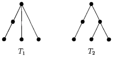
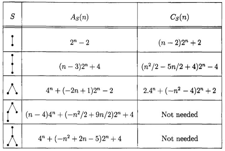
5 The expressions Ap(n) and Ст{п) 100

5.1 Recurrence relations for AT(n) and Ст(п) 100

5.2 Counterexamples to a conjecture of Kubicki, Lehel and Morayne . . . 106

6 Asymptotic behaviour of Ат(п) and Ст(п) 111

6.1 Leading terms of Ат(п) I l l

6.2 Typical embeddings of T into Tn 119

6.3 Asymptotics of the ratio At(п)/Ст(п) 122

6.4 A family of counterexamples to Conjecture 4.4 for arbitrarily large n 126

7 Results for the complete p-ary tree 130

7.1 Recurrence relations for A^\n) and C^\n) 130

7.2 The leading terms of A^\n) 135

7.3 Typical embeddings T into Tpn 139

7.4 Asymptotics of A ^ (n)/CjP (n) 141

8 Generalisations of Theorem 4.1 147

8.1 Embeddings of binary trees into the complete p-ary tree 147

8.2.1 Strict order-preserving maps 159

8.2.2 Weak order-preserving maps 163

8.3 Related open problems 166

List of Tables

List of Figures

2.1 P( 1,2;3) 48 2.2 P(1,2;3)W 48 2.3 P(l,2;3) with branching and connection points 50

2.4 Points in [ßi,ß'i\ — 4 possible cases 52

3.1 Forbidden induced suborders 67 5.1 Counterexample to Conjecture 4.4 106

5.2 Counterexample to Conjecture 4.4 109 6.1 General counterexample for d(T) > 0,d(D[y}) = 0 127

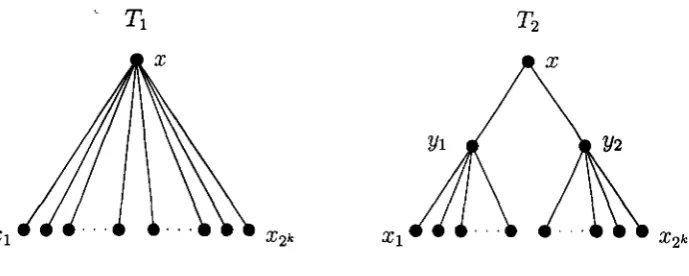
7.1 Subtrees of Ti and T2 144

8.1 The two cases for Tb+ 154

Acknowledgements

Firstly, I would like to thank Professor Graham Brightwell for his unfaltering super-vision. He introduced me to the problems studied here and he has been a constant inspiration throughout my studies. I also extend my thanks to the whole of the Mathematics Department at LSE. I have really appreciated the informal atmo-sphere around the department, and the friendly nature of all its members. I am sure that this is owing, in part, to the informal workshops and discussions at the round table—long may they continue. Particular thanks go to Dave Scott and Jackie Ev-erid for their administrative support, Mark Baltovic for his IT expertise, and my fellow research students for sharing the highlights and frustrations of research and for our many conversations on a multitude of topics, a most welcome distraction.

Away from the university, my thanks go to all my friends living in and around London who have made my time here such an enjoyable one. Special thanks go to Owen Jones, Katrine Reimers and Esme Tarasewicz for being wonderful housemates, and to Joe Walton and Nick Sample for their generosity and friendship.

My thanks, as always, to my parents and my brother, Matthew, for their loving support and encouragement.

Finally, I thank the Engineering and Physical Sciences Research Council, the London School of Economics and Political Science, and the Department of Mathe-matics for their financial support over the last four years.

Statement of originality

I declare that the work described in this thesis is wholly my own, except for the work in Chapter 3. The work described in Chapter 3 was carried out in conjunction with my supervisor, Professor Graham Brightwell and was worked on in equal proportion by myself and Professor Brightwell.

Nicholas Georgiou (candidate)

4/S

Summary

This thesis covers two areas in probabilistic combinatorics, specifically the com-binatorics of partially ordered sets. Problems and areas of study in probabilistic combinatorics broadly fall into one of two classes. The first class contains prob-lems of a deterministic nature, which are particularly suited to some application of probabilistic methods or techniques. The second class contains problems that are themselves of a probabilistic nature. We cover problems from both classes.

In the first part of the thesis we investigate a family of random models of partial orders, called classical sequential growth models. We study in detail the simplest non-trivial model from the family and analyse the partial orders it produces. We also study "continuum limits" of sequences of classical sequential growth models, proving that particular sequences of these models do have continuum limits. We also prove some results about the continuum limit of a general sequence of classical sequential growth models, when it exists.

Part I

In this part we study a family of models of random partial orders, called classical sequential growth models, introduced by Rideout and Sorkin [24]. These models were proposed as possible models for discrete space-time, since they are the only models satisfying certain desirable physical-looking conditions. In particular, we will analyse the simplest non-trivial model from the family, and we will also define and study a particular limit of a sequence of classical sequential growth models.

In Chapter 1 we give a full description of the family of models and a brief summary of the results in [24], explaining the physical-looking conditions imposed by Rideout and Sorkin, and noting that a particular model from the family can be specified by a sequence of non-negative constants.

In Chapter 2 we study in detail the particular model called a random binary growth model, showing that a random poset produced by the model almost surely has infinite (poset) dimension. This shows that, despite the simple description of the model, the random poset it produces has a complex structure. We give estimates for bounds on the size of an up-set of a particular element and show that every element in the random infinite poset is incomparable to only finitely many others. We also present a specific poset that, with some positive probability, is not contained in the random poset produced by the model. This contrasts the model with other random models of partial orders, for example the random graph order, which contains any specific poset almost surely.

Chapter 1

Introduction

We study a family of models of random partial orders, called classical sequential

growth models, introduced by Rideout and Sorkin [24]. Each model is defined on the (labelled) vertex set N, which we will always take to include 0. Any model can be restricted to [n] = {0,1, 2 , . . . , n} and regarded as a model of random finite posets. The model starts with a poset of one element (labelled 0), and grows in stages. At stage n = 1,2,..., vertex n is added to the existing poset, P„_i, by placing n above some choice of vertices of P„_i. The poset Pn is defined on vertex set [n] by taking

the transitive closure of the existing and added relations. This is called a transition from Pn-i to Pn, written Pn-\ Pn- The models are random, so each transition

occurs with some probability. These transition probabilities are fixed and depend on the particular model. Let P(Pn-i —> Pn) denote the probability of transition

Pn-i Pn occurring.

(at each stage n and for any fixed Pn-\ the sum of probabilities over all possible

transitions Pn_i —> Pn must be equal to 1). Discrete general covariance states that

the probability of producing a particular poset should not depend on the labelling of the poset, that is, given two different sequences of transitions, (Pi —> Pi+1) and

(Qi —>" Qi+i) which produce the isomorphic posets Pn and Qn, the products

n—1 n—1 П я + o a n d П ^ Gi+i)

i=0 i=0

must be equal. So, for example, discrete general covariance immediately implies that any two transitions from P„_i to isomorphic posets Pn and P'n have the same

transition probability P(Pn_i —> Pn) = P(Pn_i —> P^). Bell causality is a condition

on ratios of transition probabilities. (Note that in [24] Rideout and Sorkin only study "generic" models, meaning that all transition probabilities are non-zero, in order to make sense of this condition.) Given a particular poset P, and any two transitions P —• P', P —> P" which add the new element n, let S be the set of all elements which are incomparable with n in both P' and P". Let Q be the poset formed from P by removing all the elements of S (and obsolete relations), and define

Q' and Q" similarly. Then, Bell causality states that P(P -> P') = P(Q -> Q')

P(P P") ~ P(Q Q")'

the idea being that, since the new element is not placed above any of the elements of S in either transition, the presence of the set S should not affect the ratio of the transition probabilities.

A particular model is specified by a sequence t = (to,ti,...) of non-negative constants. The random poset is defined as the transitive closure of a directed random graph Gt on N in which all arcs go from a lower numbered vertex to a higher. The

arcs are selected sequentially, considering each vertex n in turn and choosing the set Dn С [n — 1] of vertices sending an arc to n; the probability that Dn is equal to a

A model defined according to this description is called a classical sequential

growth model. Rideout and Sorkin show that these models are the only generic models satisfying their conditions. It is an easy exercise to check that these models do indeed satisfy the four conditions; for example, Bell causality holds essentially because the relative probability that element N selects a set D, defined as t\D\, is independent of n.

Varadarajan and Rideout [31] and Dowker and Surya [12] have studied the sit-uation where the transition probabilities are allowed to be zero. The Bell causality condition becomes a condition on products of transition probabilities and the type of models that satisfy the conditions are very similar to the generic models described here.

The family of classical sequential growth models also contains models of random

graph orders. A random graph order Рпф is defined as follows. The ground set of

Pn.p is the set { 0 , 1 , . . . , n — 1}. For each pair of vertices i < j the relation (i,j)

is introduced with probability p. The poset Pn>p is then the transitive closure of

these relations. Random graph orders were introduced by Albert and Frieze [1] and have been studied further by Bollobäs and Brightwell [7, 8, 9] and Simon, Crippa and Collenberg [27]. The area is covered in the survey of random partial orders by Brightwell [10]. A classical sequential growth model defined by sequence t where

U = f for all i, and t = p/(l — p), will after stage n — 1 produce a random graph order Pn<p.

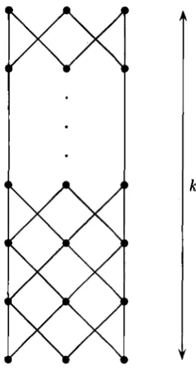
In the following chapter, we concentrate on the model where the sequence t is (0,0,1,0,...), i.e., where all U are zero except t2. This means that \Dn\ = 2 for each

vertex n. We say that n selects the two vertices in Dn. So, in this model each vertex

n selects two vertices chosen uniformly at random from the set [n — 1]. We assume that we start with the vertices 0 and 1 incomparable with probability 1 and then add vertices n = 2,3,... according to the model. (So, for example, D2 = {0,1}

random poset it produces a random binary order.

This is the simplest interesting model; the model defined by t with t0 non-zero

and U equal to zero for i > 1 produces an infinite antichain (Dn = 0 with probability

1, for all n), and the model defined by t with t0 and t\ non-zero and U equal to zero

for г > 2 produces a forest of infinitely many infinite trees, where each vertex is an upper cover of exactly one other vertex and a lower cover of infinitely many other vertices. These are called the "dust universe" and "forest universe", respectively, in

[24].

The random binary growth model also has potential applications in computer science. Under the name of a random binary recursive circuit, the random binary order has been studied by Mahmoud and Tsukiji [20, 21], Tsukiji and Xhafa [30] and Arya, Golin and Mehlhorn [4]. These papers typically focus on the "depth" of the circuit or the number of "outputs" of the circuit. These are considered as important parameters in a computer science setting; however, they correspond to the height of the random binary order and the number of maximal elements of the random binary order, which are not particularly interesting parameters of a partial order. Here we will consider parameters that are more interesting from a combinatorial viewpoint, but these will probably not have useful analogues in the recursive circuit formulation.

The random binary growth model is essentially the same as any other model with t3 — 14 = . . . = 0 since for large n the number of 2-element subsets of [n — 1]

Chapter 2

The random binary growth model

Recall that the random binary growth model is defined as follows. Start with el-ements 0 and 1 incomparable; then each element n = 2 , . . . selects two elel-ements uniformly at random from [n — 1], and we take the transitive closure. We will denote the random binary growth model by B2 and the random binary order it

pro-duces by B2. We write B2[n] for the restriction of B2 to [n] and B2[ni,n2] for the

restriction of B2 to n2] = {x £ N : щ < x < n2}.

The random binary order B2 is a sparse order; each vertex n has at most 2 lower

covers since a; is a lower cover of n if and only if it is selected by n and is not below the other vertex у selected by n. This means the Hasse diagram of B2[n] has at

most 2n edges. Also, as we now show, the expected width (i.e., the expected size of the largest antichain) of B2[n] increases with n. A vertex x in B2{n\ is maximal if

and only if all vertices у = x+l,x + 2,... ,n do not select x, so

2\ rV У - 2 ®(ж-1)

'z n

{x is maximal in B2 Ы) — I I ( 1 ]— И — /

у й Л V' 1ДД1 У n { n~l )

and so the expected number of maximal elements is

1 n 1 n

' i=2 4 ' \ж=1 i=l

= 1 (п(п + 1)(2п+1) _ w(w+ 1)\ = (n + 1)/3

(In fact, this is shown in [20], where Mahmoud and Tsukiji also show that the number of maximal elements of B2 [n] tends in distribution to a normal random variable with

mean n/3 and variance 4n/45.) The maximal elements form an antichain, so the expected width of B2[n] is at least (n + 1)/3.

However, the number of minimal elements is always 2, since only 0 and 1 are minimal. Moreover, the expected number of minimal elements of B2[ni,n2\, f°r

щ > 2, is bounded above by щ as n2 tends to infinity. Indeed, a vertex x in

B2 [fti, n2] is minimal if and only if it selects both vertices from [щ — 1], and the

probability of this is ( ^ / ( s D = ni (ni — l ) / x ( x — 1). Summing over x from щ to

n2 gives the expected number of minimal elements equal to щ — ni(ni — 1 )/n2.

In Section 2.1 we study the dimension of B2. The dimension of a poset P

on ground set X is the minimum number of linear orders on the set X whose intersection is equal to P. In other words, the minimum number of linear orders Li such that x < у in P if and only if x < у in Lj for all i. An equivalent definition is that the dimension of P is the smallest d such that P can be embedded into Rd, where Rd is the d-dimensional Euclidean space with ordering ( x i , . . . , x<j) <

( y i , . . . , yd) in Rd if Xi < yi in R, for all i = 1,... ,d. (The equivalence can be

easily proven; the essential observation is that the linear orders on X correspond to the coordinate-wise orderings of the embedded points in M.d.) Since B2 is sparse,

one might suppose there to be a relatively simple structure to B2. However, we

show this is not the case in so much as showing that B2 has infinite dimension,

almost surely. Using standard notation (see, e.g., [29]), we write P(l,2;m) for the subposet of the subset lattice formed by the 1-element and 2-element subsets of the m-element set { 1 , . . . , m} ordered by inclusion. Spencer [28] proved that the dimension of P ( l , 2; m) is greater than log2 log2 m, so we show that B2 has infinite

directed random graph Gt).

In Section 2.2 we study the sizes of up-sets in B2[n] and, related to this, the

number of elements in B2 incomparable with an arbitrary element. Although B2 is

sparse, we show that for all r the number of elements incomparable with r is finite. In particular, this implies that B2 does not contain an infinite antichain, almost

surely. Moreover, for any classical sequential growth model defined by sequence t where U ^ 0 for some i > 2, the same result is true, that the random poset produced does not contain an infinite antichain, almost surely.

We use the differential equation method of Wormald [32, 33] which specifies when and how a discrete Markov process can be closely approximated by the solution to a related differential equation. We prove a version of Wormald's theorem which makes explicit the errors in the approximation. We use this result to analyse the growth of the up-set of an arbitrary point. For a fixed point r, write for the set of elements above r in the finite poset B2[n}. We can think of "growing the poset"

by increasing n. Then |С4П'|, which depends on n, can be considered as a Markov

process. Using this "differential equation method", we give good estimates on for particular values of n, and show that there exists an n = n(r) such that Ir С [п].

Here, Ir is the set of vertices greater than r which are incomparable with r. So, for

fixed r, there are no vertices greater than n incomparable to r, and so the number of vertices incomparable with r is finite. We provide two similar proofs, one giving bounds for a typical r, and one giving bounds for all but finitely many r.

Is the fact that P(l,2,ra) is almost surely contained in B2 a special case of

something more general? Is it possible, as in the case of random graph orders, that

every finite poset is contained in B2, almost surely? In Section 2.3 we show that this

is not the case. We use our result from Section 2.2, that there is an n = n(r) such that for all but finitely many r, there are no vertices greater than n incomparable with r. So, we know that if two elements in B2 have labels with a large enough

in B2 must have two elements whose labels have large difference. Combining these

two results, we provide an example of a poset not contained in B2 (or rather, there

is a positive probability that B2 does not contain the poset).

2.1 The dimension of B

We write P(l, 2; m) for the subposet of the subset lattice formed by the 1-element and 2-element subsets of the set { 1 , . . . , m} ordered by inclusion. For a particular vertex r, let Ur be the set of all vertices above r in B2 and let ufi be the set of all

vertices above r in B2[t]. Denote by Tk the hitting time of the event \Ur\ — k, i.e.,

the smallest t such that = k, and the waiting time between events \Ur\ — к — 1

and \Ur\ = к by Wk, so that Tfc+1 = Tk + Wk+i- We include the point r in Ur so

that Ti = r.

We now show that, for every m, there exists a copy of P( 1,2;m) in B2, almost

surely. This is enough to show that B2 almost surely has infinite dimension, since

dimP(l,2;m) > log2log2m (see [28]).

In fact, we will prove a stronger result, that for each m there exists an r0 such

that the probability of there being a copy of P(l, 2; m) in B2[r, 2r1^} is greater than

3/5 for all r >

Го-We use the following lemma to find a copy of P(l, 2; m) in B2[r, 2r7/5].

Lemma 2.1. For any m, and any щ < n2, if we have sets X = {xi,... ,xm} С

[ni,n2], Y = {yi,... ,ум} ^ where M = and the following conditions

hold

(i) the points in X are incomparable in ^[ni, n2],

(ii) for each pair of points CC j j CCj %rf\ X there is exactly one yk in Y which is above

then X U Y is a copy of P(l, 2; m) in В2[щ,п2] where X is the set of minimal

elements and Y is the set of maximal elements.

Proof. Let < be the order on В2[п\,п2]. To show that X\JY is a copy of P(l, 2; m)

we need to show that the only relations are those described by condition (ii). That is, that there are no relations of the form Xi < Xj, yk < yi or yk < X{.

By condition (i) there are no relations of the form So, suppose there exists some relation Ук<Уь Since \Y\ = M = (™), condition (ii) implies that there exists a pair Xi, Xj with xi? Xj < yk. But then ж», Xj < yi contradicting condition (ii).

Suppose there exists some relation у к < Xi. Then by condition (ii) there exists some

yi with Xi < yi. But then yk < y% which leads to a contradiction as above.

So, X U Y is a copy of P(l, 2; m) and X is the set of minimal elements and Y is

the set of maximal elements. •

Proposition 2.2. For every m, there exists an ro such that the probability of there

being a copy of P( 1,2; rri) in B2[r, 2r7/5] is greater than 3/5 for all r >

ro-Proof. We will prove the result as follows. Assume that m is fixed, ro is sufficiently large and r > r0. First we find a set of points that satisfies condition (i) of Lemma 2.1

with some high constant probability. Because of the sparsity of B2, it is easy to find

this set. Here we will take the points r,r + 1,... ,r + m — 1. These points will form the minimal elements of a copy of P ( l , 2; m). We then grow the poset up to size r7/5,

keeping track of the sizes of the up-sets of these chosen minimal points. The value r7/5 is chosen so that the up-sets are large enough, but their pairwise intersection is

still an insignificant fraction of the whole up-set. This means that the set of points above one and only one of the minimal points is reasonably large. The bulk of the proof is in showing this. Finally, we grow the poset up to size 2r7/5 to find the points

satisfying condition (ii) of Lemma 2.1. Indeed, we look for points in [r7/5 + 1,2r7/5]

points is at least some constant probability. We then apply Lemma 2.1 to obtain the result.

Following this scheme, where m is fixed, ro is sufficiently large and r > ro, consider the points r, r + 1,... ,r + m — 1. We attempt to find a copy of P(l, 2; m) in which these are the minimal elements. We have,

m—l /r\

P(r, r + 1,..., r + m - 1 are incomparable) = JJ jgl- > 9/10 for rQ > 20m2.

i=1 \ 2 )

Now grow the poset by adding points up to n = r7/5. We consider the growth

of the set Ur- We calculate the expected waiting time EWk+i as follows. Suppose

Tfc = i, then since Wk +i always takes integer values greater than or equal to 1 we

have

00 00 j /t+l-k\

ЕИ4+1 = 1 + J > ( W_{j=1 j=1}f c +i > j ) = 1 + J ] П " S b r _{1=1 V 2 )}

and using the inequalities 1-х <e~x and f{x)dx < / ( j ) < f^ f(x)dx,

for / decreasing, we have

oo j /t+l-k\ OO / j

w . ^ i + E I l W f + E П

2

Cr) " t + i

J=1 \ 1=1

°° ( P + X 1 \

< l + g e x p [ ~ 2 k Jt — d l )

f + 1 V *

= 1+Е(щтт]

f°° 1

<1 + ( t + 1 )- yo

(t + l)2k 1

= 1 + That is,

E(Wfc+i|Tfc) < 1 +

(t+l)2k~1 2k-1'

Tk + 1

2k-1

So, we have

/ ET1 4-1\ 2 к

which by induction on к gives

ETfe+1< (22k /(2k))r + 2k. (2.2)

Using Stirling's approximation we have

/ 2 k\ V2ir(2k)2k+1/2e-2k+1tt24k+V 22k+1/2e1^24k+1^

\k ) ~ (^fefc+l/2e-fc+l/12fc)2 ~ ^fcl/2el/6fe ' f 0^ ^1 '

so ETk+i < + 2k, for к > 1. For к > 2, ^£ei/e*-i/(24fe+i) < 2

and using (2.2) we have ET2 < 2r + 2, so ETk+i < 2r\[k + 2k and so

ETk < 2rVk + 2k. (2.3)

If we similarly define Ur+l, T ^ , for r + г, г = 1 , . . . , rn — 1 and write for

Tk, then we have T^ = r + г, giving equations

Е Т «1< ( 22 А/ © ) ( г + г) + 2А;, (2.5)

ETf < 2(r + i ) Vk + 2k, (2.6)

corresponding to equations (2.1),(2.2) and (2.3).

For r0 > m we have r + г < r + m < 2r, so (2.6) becomes

ETfc(i) < + 2k, i = 0 , . . . , m - 1.

So, recalling that n = r7//5, we have

P(|C/j"l| < r3 / 4) = P(Tr 3/ 4 > n) < E Tr 3/ 4/ n

< (4Г11/8 + 2r3 / 4)/r7/5 < 6/r1/40 < l/10m

for r0 > (60m)40, and similarly for г = 1 , . . . , т - 1 .

Therefore, P(all |c4n]|, • • -, > rz'A) > 9/10.

We say a point a; selects a pair of sets (Xi,X2) if Dx = {:ri, x2} for some x\ e Xx

bounds on uj^i we can show that, with high probability, there exist points in B2 [2n]

selecting each pair ( U ^ , U ^ ) . We might hope for these to form the maximal points of a copy of P( 1,2;m), since for each pair of minimal points r + i,r + j we have a point above both. However, it is possible for these potential maximal points to be above more than 2 minimal points. We need to find points above exactly 2 of the minimal points. To do this we need to look at a subset of Ur+i, namely the set of

points above r + i but not above any other r + j for j Ф i.

For points x, у in B2, write Uxy for the set of points above both x and y. Consider

the restricted poset B2[n] and write ut'y for the set of points in B2[n] above both x

and y. We will show that is small in comparison to |f4"'| and Call a sequence of integers (i,)*=1 from [r, n] a path if ij selects ij-\ in the poset, for

j = 2 , . . . , s. So a path is necessarily a strictly increasing sequence. We say a path

(b)j=i is fr°m 4 to is. Define a forked path with ends x,y, z and connection point

w to be three paths, one from x and one from у both to w, and a third from w to z (so x, у < w < z), with w the only common point of the first two paths. Note that we allow the possibility that w = z, in which case the third path is the single point

w = z.

For each point и in there must be paths Pr from r to и and Pr+1 from

r+1 to щ if we set v = min{j : j is a common point of Pr and Pr+i} then by taking

the subpath (subsequence of consecutive terms of a path) from r to v (of Pr), the

subpath from г + 1 to и (of Pr+i) and the subpath from v to и (of either Pr or

Pr+1) we have a forked path with ends r,r + 1 and u, and connection point v. This

forked path is not necessarily unique, since Pr and Pr +i are not necessarily unique.

Let FP(r, r + l,v) be the total number of forked paths with ends r and r + 1 and connection point v all fixed, and with arbitrary third end u, with v < и <n. Let

FP(r, r + 1) = J2v=r+2 F P г + 1, «)• Then \Urr+i\ < FP(r, r + 1).

Now, the probability that a strictly increasing sequence is a path in B2[n]

We can also calculate the probability that the points {г0,4, • • •, is}, i0 < i\ <

•••< is form two disjoint paths in B2 [n], one from г0, the other from ii, as follows.

Start with two sequences A — (г0) and В = (ii), then taking each point ij,j =

2 , . . . , s in turn make it the next term in either sequence A or sequence B. (So, the resulting A and В are disjoint subsequences of (ij)j=0)- The probability that we

can make A and В paths is the probability that at each step ij selects one of the current end terms of A or B. For step j this is at most 4/ij so by independence the total probability is less than П^=2(4/г^). We have inequality here because we are

over-counting the case where ij is above both of the current end terms of A and B. The expected size of FP(r,r + 1, v) is the sum over all subsets I of [r, n], with r,r + l,v G / , of the probability that I forms a forked path with ends r, r + l , m a x l and connection point v. This is the probability that I<v = {г €

I : г < v} forms two disjoint paths from r and r + 1; and v selects the end of both paths; and />„ = {i e I : i > v} forms a path from v to max/. So, for / = {r, r + 1,г2,.. - ,is-i,v,is+i,... ,is + s/} with ij increasing and r + 1 < г2,

is~i < v < is +i this probability is less than x 1 / g ) x

UU^M-So the sum over all such subsets I can be written as the following product, since the individual terms of the expanded product correspond exactly to the required probabilities for all subsets I,

~ \r + IJ v(v-l) w 2 n2

using the inequalities 1 + x < ex and =a /(г) < Ja6_1 f(x)dx for / decreasing, so

in particular Ya=o. 1Д < log 6 - log (a - 1).

E F P ( r , r + 1) < 2r1/5. The same method gives the same upper bound on the

expected size of U^y for all pairs (x, y) in [r, r+m— 1](2) so P(| ü M j > (10 m2)rl'b) <

l/5m2 and P(all |c4nJ| < (10m2)r1/5) > 9/10.

Let Ain' be the set of points above r but not above r + 1 , . . . , r + m — 1 in B2[n],

then 4n l = Uln] \ UI^1 Similarly define A[?\ x e [r + 1, r + m - 1]. Then,

for v > r0 > 400m6, we have (10m2)rlj/5 < r3^/2m so with probability greater than

4/5 we have all \A[x]\, x € [r,r + m - 1] at least |r3/4.

We grow the poset by adding a further n = r7/5 points, to find our maximal

points: M = points ai,... ,ам, so that each pair of sets (Ai"', A^'), {x,y) S r, r + m — is selected by some a*.

Now,

1 4 M 1 1 4 M I „3/2 „ 3 / 2

P(» + i selects ( 4 " U " i ) ) = > > ~ b, i < n,

so

/ r3/2\

P(none of n + 1 , . . . , 2n selects (Aj.n], АД1)) < ( 1 - ^ )

< exp(-r1/1 0/8),

which is less than 1/10M for r0 > (8 log 10M)10. The same calculations give the

same upper bound on the probability of failing to find a point in [n + 1,2n] which selects for each (x,y) £ [r,r + m — _{so the probability of failing to} find points a i , . . . , ам in [n + l,2n] as desired is less than 1/10.

So with probability at least 3/5 we have sets { r , r + l , . . . , r + ra — 1} and { ab a2, . . . , aM} satisfying the conditions of Lemma 2.1. Therefore {r,r+ 1,... ,r +

m - 1, ai, a2,..., aM} is a copy of P( 1,2; m) in B2[r, 2n], •

Theorem 2.3. For every m there exists a copy o / P ( l , 2 ; m ) in B2, almost surely.

To find a copy of P( 1,2; m) in B2 we split B2 into disjoint sets of the form B2[nx,n2)

as follows.

For i = 1,2,..., let ri = 2r7£ + 1. By Proposition 2.2 the probability of there

not being a copy of P ( l , 2 ; m ) in В2[г{)2г7/5] is less than 2/5, for each i. The

probability of not finding a copy of P ( l , 2 ; m ) in the infinite poset B2 is less than

the probability of not finding a copy of P ( l , 2 ; m ) in every poset В2[г^2г7,ъ\. But

the sets В2[г^2гУ5} are disjoint, so the events "not finding a copy of P(l,2;m) in

B2[ri, 2rJ^5]" are independent. Therefore the probability of not finding a copy of

P(l, 2; m) in the infinite poset B2 is zero, as required. •

Corollary 2.4. B2 has infinite dimension, almost surely.

Proof. This is immediate, since dimP(l,2;m) > log2log2m. •

This tells us that, almost surely, there is no finite d such that B2 can be embedded

into Rd, the d-dimensional Euclidean space with ordering ( x i , . . . , xa) < (j/i, • • •, Уа)

in Rd if X{ < yi in R, for all i = 1,..., d, as defined earlier. What can be said for

embeddings into other partial orders? Since classical sequential growth models have been proposed as possible models of discrete space-time it would be interesting to know whether the partial orders they produce can be embedded into a rf-dimensional Minkowski space for some finite d.

The Minkowski space Md is defined as the partial order on Rd with ordering

(x0,..., xd. i) < (y o , yd- i) in Md if y0- x0 > у ( i / < ~ ®02 in The

Minkowski dimension of a partial order P is the smallest d such that P can be embedded into Md. It is known that a finite partial order P can be embedded into

Md+1 if and only if P can be represented as a d-sphere order. A c?-sphere order is

a partial order on a ground set of spheres in Rd, with the ordering on the spheres

most 4, for all m.

We believe that the random binary order B2 has infinite Minkowski dimension.

A proof of this result could follow the proof strategy of Theorem 2.3; find a family of partial orders with arbitrarily large Minkowski dimension that are almost surely contained in B2. Unfortunately, the partial orders known to have large Minkowski

dimension are all significantly more complex than P(l, 2; m). Given the complexity of the proof of Proposition 2.2 it would be ambitious to attempt a proof using this strategy. Instead, we make the following conjecture.

Conjecture 2.5. B2 has infinite Minkowski dimension, almost surely.

We justify the conjecture as follows. If the poset B2 has finite Minkowski

dimen-sion, then it can be embedded into Md for some d. Since the model B2 produces the

poset B2 sequentially, this means that at each stage n the finite poset B2[n] can be

embedded into Md. However, this seems unlikely since at each stage the element n

selects two existing elements at random, each pair of elements being equally likely with no regard to the existing structure of the embedding of B2[n — 1] in Md. It

seems more likely that the random nature of the model B2 is such that, for large

enough n, the poset B2[n] produced at stage n cannot be embedded into Md.

2.2 Up-sets of vertices in B

Brightwell [11] proved that, almost surely, each element of B2 is comparable with

all but finitely many others. This result is contained within what we prove here; we need a more refined version, providing an estimate of the number of elements in B2[n] that are incomparable with an element r, and an estimate of the largest

element incomparable with r. Recall that U|nl is the up-set of r in B2[n] and that

use these estimates to provide estimates of the size

In [32, 33], Wormald presented a theorem which describes when and how a dis-crete time Markov process can be approximated by the solution to a related differ-ential equation. However the approximation is only in terms of asymptotic bounds; here we state and prove a version of the theorem which gives explicit expressions for the approximation.

We begin with some definitions.

Definition 2.6. A function / : R2 —> R satisfies a Lipschitz condition on a

con-nected open set P C R2 if there exists a constant L > 0 with the property

for all (xi,yi) and (£2,2/2) in V.

Definition 2.7. For У a real variable of a discrete time random process Go, Gi, •. • which depends on a scale parameter n, we write Y(t) for Y(Gt), and for a connected set P C R2 define the stopping time Tv = TV(Y) to be the minimum t such that

Definition 2.8. A sequence of random variables Yo, У , • • • is a martingale with respect to a sequence of сг-algebras f o ^ f i С . . . if, for all i,

(i) Yi is .^-measurable, (ii) E|Yi| < 00,

(iii) E(yi +i I Ti) = Yi almost surely.

If, instead of (iii), we have:

• E(yi +i I Ti) < Yi almost surely, then (Уг) is a supermartingale with respect to

• Е(Уг+11 Ti) > Yi almost surely, then (Уг) is a submartingale with respect to

№ ъ Ы ~ f ( x 2,2/2)1 < Ц\хх - x2\ + I yi - 2/2I) (2.7)

The following lemma will be used in the theorem and is a simple extension of a martingale inequality, known as Azuma's inequality [5], to supermartingales. We omit the proof, which can be obtained by an obvious modification to the proof of Azuma's inequality.

Lemma 2.9. Let lo> Yb ... be a supermartingale with respect to a sequence of

a-algebras Q Q • • • with JF0 trivial, and suppose Y0 = 0 and \Yi+i — < с for

i > 0 always. Then for all a > 0,

РФ > ас) < exp (—a2/2i).

We are now in a position to state and prove our version of the theorem.

Theorem 2.10. Let Y be a real-valued function of the components of a discrete time

Markov process {Gt}t>o- Assume that V С R2 is connected, closed and bounded and

contains the set

{(0, y) : P(Y(0) = yn) 0 for some non-negative integer n}

and

(i) for some constant ß,

\Y(t + l)-Y(t)\<ß

always for t < Tv,

(ii) for some function f : R2 —> Ж which is Lipschitz with constant L on some

bounded connected open set Vq containing V, and some constant X,

|E(Y(* + 1) - Y(t)\Gt) - f(t/n, Y(t)/n)I < X/n

for t < Tv,

(in) f : R2 —> R is bounded on VQ, i.e., there is a constant 7 such that \f(x,y)\ < 7

T>o-Let w = w(n) be a fixed integer-valued function with w = o(n). Then the following

are true.

(a) For (0, у) 6 V the differential equation

t x

^

has a unique solution у = y(x) in V passing through y(0) = y, and which extends

for some positive x past some point, at which x = a say, at the boundary ofD;

(b) Writing i0 = min{\Tv/w\, [an/wJ} and ki = iw, there exists some В > 0 such

that

P(|Y(£) - ny(t/n)I > Bt + {ß + i)w) < 2ie~2w3/n2

for all i = 0 , 1 , . . . , г'о — 1 and all t, ki <t < ki+i, and for i = iQ and h0 <t <

min {Tu, an), where B{ = ((1 + Lw/n)г — l)Bw/L, and y(x) and a are as in

(a) with у = Y(0)/n.

Proof. Following the proof in [32], we have part (a) from the theory of differential equations. Let y(x) and a be as in part (a).

Let 0 < t < T-p — w and let 0 < к < w. This implies that t + к < T-p and so \ n ' n '

By (i), we have \Y(t + к + 1) - Y(t + k)\ < ß. Also, by (ii),

E(Y(t+k+l) - Y{t+k)\Gt+k) < f + ^

<!&

)

J \n n J n

(

. , (t_ Y(t)\ L(w + ßw) + X

\n' n ) n

where the second inequality follows from (2.7). Writing g(n) for (L(w +ßw) + \)/n, the inequality becomes

E(Y(t + k+l)-Y(t + k)\Gt+k) < f ( - , + g(n).

Therefore, conditional on Gt,

Y(t + k)~ Y(t) - kf ( - , Ш-) - kg(n) \n n J

is a supermartingale in к with respect to the sequence of cr-fields generated by

Gt>. •., Gt+W. The differences of the supermartingale are, by (i) and (iii), at most

ß + f +g(n) < ß + -r + g(n). _{V ТЬ Tt J}

So, by Lemma 2.9, for all a > 0,

P[Y(t + w)~ Y(t) - «,/ ( l Ш) - wg(n) >a(ß + 1 + g{n))) < e^^. (2.8)

The same argument with

Y(t + k)~ Y(t) -kf(~, Ш-) + kg(n) \n n J

a submartingale gives

P[Y(t + w)~ Y(t) - wf ( i , HÜ) + wg(n) <~a(ß + 7 + g(n))) < e~a''2w. (2.9)

Setting a = 2w2/n and combining (2.8) and (2.9) gives

Р(|У(* + w) - Y(t) - w f f a Z ? ) I > 2(w2/n) (ß + 7 + g(n)) + wg(n)) < le'2^^. (2.10)

Now, define k{ = iw, i = 0,1,..., i0 where i0 = min {\Tvlw\. [an/w\}. We

show by induction that for each such i,

P(|y(fci) - y(ki/n)n\ > Bi) < 2ге-2*'3/"2 (2.11)

where Bt = ((1 + Lw/n)1 - 1 )Bw/L for some В > 0.

So, assume (2.11) is true for i. Write

Ai = Y(ki) - y(ki/n)n

A3 = Y{hi+1)-Y{ki)

A3 = y(ki/n)n - y(ki+i/n)n

The inductive hypothesis (2.11) gives |Ai| < Bi with probability at least 1 -2ie~2w3/n2. By (2.10) we have

\A2 - wf(ki/n, Y(ki)/n)\ < 2(w2/n)(ß + 7 + g(n)) + wg(n)

with probability at least 1 - 2e~2w*/n2.

Since / satisfies the Lipschitz condition and (ki +i/n,Y{ki +i)/n) € V (because

ki+1 < Tx>), we also have

Из +wy'(ki/n)\ = Iy(ki/n)n - y(ki+l/n)n + wy'(ki/n)\

= I-wy'(k/n) + wy'(ki/n)I for some k, h < к < ki+i

= w\f(k/n,y(k/n))-f(ki/n,y(ki/n))\ since у is solution to (a)

< wL [w/n + Iy(k/n) - y(ki/n) |] by (2.7)

< wL[w/n + (w/n)\f(k'/n,y(k'/n)) |] for some к', h<k' <k

< wL [w/n + {w/n)7] by (iii)

= L( 1 + 7 )w2/n

where we have used the Mean Value Theorem (twice, to get lines 2 and 5). So,

Wih/n)- f{ki/n,Y{ki)/n)\ = \1{к/щу(^/п)) - f{ki/n,Y{ki)/n)\ < ЦА^/п

and so assuming \Ai\ < Bi, we have

|Лз - ( - » / № / » , Y(K)/n))I < a i ± 2 i « ! + to < + + toД.

So, we have

IY{ki+l) - y(ki+1/n)n\ = \Ai + A2 + A3\

<Bi + 2 (w2/n) (ß + 7 + g{nj) + wg(n) + L( 1 + 7)w2/n 4- BiLw/n

= [2{w2/n) (ß + 7 + g{n)) + wg{n) + L( 1 + 7)w2/n] + Д ( 1 + Lw/n) (2.12)

with probability at least 1 - 2 ( i + l)e~2w3/n\

There exists В > 0 with

2(w2/n) (ß -f 7 + + + L( 1 + 7)w2/n < 5 w2/ n (2.13)

for all n, so the term on the right hand side of inequality (2.12) can be replaced with Bi( 1 + Lw/n) + Bw2/n, which is exactly Bi+1_. So we have (2.11) for г + 1.

Finally, ki+\ — ki = w and the variation in Y(t) when t changes by at most w is

at most ßw, by (i), and as before \y{ti/n)n — y{t2/n)n\ is less than w\f(t/n,y(t/n))\

for some t, ti < t < t2 and this is less than jw. So

V(\Y(t) - ny(t/n)I > Bi + {ß + y)w) < 2ie~2w3/n2

for all i = 0 , 1 , . . . , г'о — 1 and all t, ki < t < ki+1, and for г — io and kio < t <

min{Tx>, an}. • We can apply Theorem 2.10 to \uln^\ as follows. We take as the Markov process

the random binary growth model, and as the real-valued function the size of the up-set of a fixed vertex r. We then find sets V and Vo, a function / , and constants

ß, Л and 7 satisfying the assumptions of the theorem. We obtain the following corollary, which shows fairly precisely how grows as m goes from some initial

n to [a + 1 )n, where a is a large constant. Over this range, \U^\/n grows from a small value to a value near to 1.

Corollary 2.11. For fixed r and any n> r, if = c(n)n for c(n) an arbitrary

function of n, then

a + i

P

for any constants 0 < 5 < 1/3, a > 0.

Proof. Fix a vertex r in B2[n}. Let the Markov process {Gt}<>o be the random

binary growth model but starting at stage n, so that Gt corresponds to B2[n +t].

Let Y(t) be the size of the up-set of r in B2[n + t], i.e., Y(t) = |f/]n+il|. For any

constant о-, define V as the region {(x, у) : 0 < x < о, 0 < у < x + 1}. The region

T> contains the interval {(0,у) : 0 < у < 1}, and since = c(n)n, we must have c(ri) < 1 for all n. So, V satisfies the assumption in Theorem 2.10, since it contains all points (0, c(n)) for n = 1 , 2 , — We now find a set T>0, a function / ,

and constants ß, Л and 7 satisfying assumptions (i)-(iii).

Since Y(t) = \uln+t]\ < n+t we have Y(t)/n < t/n+1, and so (t/n,Y(t)/n) E V

as long as t/n < cr. This implies Tv = \on\ + 1.

Let ß = l, then (i) holds since \Y(t +1) - У(4)| = |^n+t+1]| - < 1 always

for t < an.

Let f{x,y) = 2y/(x+l)-y2/{x+l)2. Let L = 2.1 and 7 = 1.1. The function /

is bounded on V by 1 (attained when у = x+1) and is continuous over the boundary of V, so there exists an open set V containing V on which / is bounded by 7 = 1.1. Also, ||V/||, the length of the gradient vector of / ( V / = is bounded on P by 2 and is continuous over the boundary of T>, so there exists an open set T>" containing V on which ||V/|| is bounded by L = 2.1. But then

| / ( u) - / ( v ) | < L | u - v | (2.14)

of the two sets V, V". So, (iii) holds, and (ii) holds with Л = 1, since

E(Y(*+1) - Y(t)|Gt) = 0 x P(Y(t+1) = Y(t)\Gt) + 1 x P(Y(*+1) = Y(t) + l|Gt)

= г _ (n + t+l-Y(t))(n + t-Y(t))

(n + t + l)(n + t)

= 2Y(t)(n + t+l)-Y(t)(Y(t) + l)

{n + t + l){n + t)

which differs from f(t/n, Y(t)/n) by at most 1/n for t < an.

Now T-d — [an\ + 1 and so Tv > an. So Theorem 2.10 gives the result (b) for

г = io, t = an, namely that, for some В > 0,

P(|Y(<m) - ny{a)\ > Bio + 2.1 w) < (2.15)

Here у (x) is the solution to the differential equation

V y 2

dx x + 1 (x + l)2

with initial condition y(0) = c(n). This is a homogeneous equation with solution

I

N-У [ х )~ х+1/с(пУ

Also, i0 < an/w, so Bio = ((1 + Lw/n)io - 1 )Bw/L < BweLa/L, and (2.15)

be-comes

P \uln+<Tn]\

-ri-ff + l/c(n) for some В > 0.

> Bweba/L + 2.1^ < 2(an/w)e —2w3/n2

Choose <5 with 0 < 6 < 1/3 and set the arbitrary function w(ri) to n2/3+<5. Then

w(n) = o(n) and so using the particular values for L, /3,7 and Л, we can satisfy

equation (2.13) with В = 21 and this gives the required result. • In the proof of Proposition 2.2 we bounded the expectation of the hitting time

of the event \Ur\ — k. We use this bound to show that Ur contains all but finitely

Theorem 2.12. For any constants e, rj with 0 < e < 1/4 and 0 < 77 < 1 there exists

r0 such that for all r > r0 both \Ir\ < r2+4e and Ir С [r,r4+8e] hold with probability

at least 1 — 77.

Proof. Assume that r is sufficiently large. As before, let Tk be the hitting time of

event \Ur\ = k, in terms of the growth model, i.e., the smallest t such that |Uf1 \ = k.

As in (2.3), we have ETk < 2ry/k + 2k. So E7> < 4r2 and Markov's inequality gives

P(( C/[(i6/^]| < r2j = p ^ > (i6 / 7 ?)r2) < ^ ( 2 1 6 )

so that with suitably high probability the size of the up-set, \Ur16^r2\ is at least

fraction ?7/16 of the size of the poset, (16/?7)r2.

Set щ = (16/т7)г2. We can rewrite equation (2.16) as

F(\Ulno]\/n0 > nj 16) > I-77/4. (2.17)

Assume we have \ulno]\/n0 > 77/I6. Let г be an arbitrary constant with 0 < e <

1/4. We will use Corollary 2.11 to show that as the size of the poset, тг, increases from щ to (<7 + 1)тг0, for some constant a, the ratio \U^\jn also increases, to a

value that is at least 1 — e/2.

i[/Mi

Claim 2.1. There exists a constant o0 (dependent on e and r/) such that if—-—- >

Щ

,jy[(<T0 + l)n0]|

77/I6 then r — - > 1 — e / 2 with probability at least 2<уощ e~2no .

(£70 + 1)тг0

Proof of Claim 2.1. Suppose |[/]"о1|/^о > Г7/16. Applying Corollary 2.11 with

n = n0, c(n0) = 77/I6 and S — 1/12 we have \Ulno(<T+1)]\ <7 + 1

P

n0(<7 + 1 ) CT + I6/77

for any a > 0. Set a0 so that

ffo + 1

/ 10e21<7 + 2.1 \ 1 \ 1 / 4 -1/4 ,

-v g+1 )^)-

2anle (2Л8)

/10е21<т° + 2.1\ 1

and then for sufficiently large r, - — - j - < e/4. Combining this

V ao + 1 J nQ'

inequality with (2.18) and (2.19) and setting a = <r0 gives the result. •

Let M = (l6/rj)(a0 + 1), so that (cr0 + l)n0 = Mr2. We have shown that, with

suitably high probability, \uln\/n > 1 — e/2 for n — Mr2. We now show that

\Uln]\/n remains close to 1 for all larger n. That is, that \U^\/n > 1 — e for all

n > Mr2.

Let n\ = Mr2, and щ = (1 + e/2)i _ 1ni for i = 2,3,

Claim 2.2. If\ulni]\/rn > 1 -e/2 then

(a) \Uln]\/n >1 — e for n = щ + 1,щ + 2 , . . . , |ni+ij and

(b) \ulni+l]\/ni+1 > 1 - e/2 with probability at least 1 - еп)/Ае'2п^.

P r o o f of Claim 2.2. Suppose we have |f4nil \/щ > 1 - e/2.

For part (a) we use the fact that is increasing in n, so that

\uln]\ > \uini]\ _ \ulni]\ > l - e / 2 > 1

n ~ ni+1 (1 + е/2)щ ~ 1 +e/2 ~ £

for all n = щ + 1, rii + 2,..., [ni+1\.

For part (b) we apply Corollary 2.11 with n = щ, a = e/2 and S = 1/12. We have

\ U ln i { £ / 2 + l ) ]\ г / 2 + l

P

щ(е/2 + 1) e/2 + 1 /с{щ)

with с(щ) > 1 - e/2. So,

A O e ^ ^ n W 1/4 ,

£/2 + 1 J n y 4 , - K

(2.20)

e/2 + 1 e/2 + 1

e/2 + 1 /с{щ) - e/2 + 1/(1 - e/2) and for sufficiently large r,

e/2 + 1 _ /I0e2-W2 + 2.1\ 1

Then, (2.20) becomes < 1 - e/2) < en],Ae~2n''A. •

Notice that, since ni+1 > щ, if the inequality (2.21) is satisfied for i — 1, then it

is automatically satisfied for all larger i. That is, if we have r sufficiently large to be able to apply Claim 2.2 once, then we can apply it repeatedly to get the following.

Assuming ]t/]nil|/ni > 1 — e/2, we have \U^\/n > 1-е for all integers п>щ =

Mr2 with probability at least 1 - X ^ i erh'^4е~2п*', for sufficiently large r.

Let r be sufficiently large so that 2a0n0 / 4e-2 no4+YaLi еп/4е~2п¥4 < tj/4. Then,

we have \U^\/n > 1 — e for all integers n > Mr2 with probability at least l — rj/2.

Once \uln]\ is always a large fraction of n, we can show that C/jn' becomes almost all

of the poset B2[n] for n — r4+8e. Rather, we now look at lln\ the set of points in

[r, n] incomparable with r in -B2[n].

For t > Mr2, set st = \1^\/уД, and consider the sequence (st) as a stochastic

process.

We have that

I stj ( L with probability 1 - C f O / C t1)

st+i = <

[ ^ with probability ( I f I) / C+1)

Therefore

St-Ji+

Cf

)/('?)

_

ГГ

/

= — = 4—111 + t(t+1)

Now, provided st < е\Д (which will be the case unless \U®\ drops below (1 - e)t),

we have

for all t > Mr2. So

< ( Mr2 + 1 \1 / 2~£

- 4 \ Mr2 + k + 1J

( Mr2 + 1

4 \Mr2 + k+1

where we have used the fact that e < 1/4 to get the last line. So,

Using Markov's inequality, we have sr4+se < (4/77)M1_£r_2£+8e2 with probability at

least 1 — 77/4.

Therefore |4r4+8e]| < V ^ . { 4 / r i ) Ml-£r ~2^S £ 2 = Mr2 + 2 £ + & 2 with probability

at least 1 - 77/4, where M = (4/?7)М1_г.

Finally, let us consider the probability that all vertices with a label higher than

r4+8e a r e comparable with r; in other words /,И = if + ^ for s > r4 + &. Given the

size I i t + this probability is exactly

77/4. Also, |4r4+8S]| < Mr2+2e+8e2 < r + , for sufficiently large r. So, combining all

This result is close to the best possible; as the following lemma shows, we have that E|t4n]| < n2/r2, so for small e > 0, \Ir \ > r2~e with high probability.

Lemma 2.13. For all n>r, E|c4n]| < n2/r2.

which is at least

the probabilities, we have |/r| = \Ir

at least 1 — 77, as required.

[r4+8e] _{< r}

2 + 4 e and Ir С [r, r4+8e] with probability

Proof. Firstly, we make an observation similar to that in the proof of Proposition 2.2 on page 26, that for all и e U ^ there must exist a path from r to u. Therefore, it is enough to provide an upper bound on the expected number of paths in B2[n]

with start point r. As before, for r < ii < i2 < • • • < is, the probability that

{ г , ц , г2, . . . ,г8} is a path is

s a 2 P(ii selects r) selects ij-\) = J"J —.

j=2 j=i гз

So, the expected number of paths in B2[n] starting at r is bounded above by

£ P ( { r } U / i s a p a t h ) = £ П т = П ( 1 + 7 ) /С[г+1,п] /С[г+1,п] iel i=r+1 ^ '

= ( w + l ) ( n + 2)

~ ( r + l)(r + 2) - r2' •

We have shown that for a typical r, the size is a constant fraction of n for n = ©(r2), and that the set Ir is contained in [r4+8e], with \Ir\ = 0(r2 + 4 e). What

about for a worst case r? Can we say something about all but finitely many r?

Clearly, we cannot always expect | U ^ \ to be a constant fraction of n for n = 6 (r2). As we showed in Section 1,

t(T

n(n — 1) which is approximately r2/n2. Setting n = r3/2, we have that

P(r is maximal in B2[r3/2]) « ^

which means there are infinitely many r with |f4r3/2]| = 1. When this is the case,

the growth process of for n > r3/2 is identical to the growth process of

for n > r3//2, since the sizes of U[f2] and U[ 3/2' are the same. So, the expected size

of can be found by substituting r3//2 for r in Lemma 2.13, which shows that

E|f4n'| < n2/(r3 / 2)2 = n2/r3. So, for such an r the expected size of U^ ' is less than

r, and we need n = 6(r3) before the expected size of f/|n' is a constant fraction of n.

and then Ir is contained in [r6+£'j, with \Ir\ = 0(r3+£). Heuristically, it appears that

the growth of |c4n'| is highly dependent on the values of the hitting times, for

small к, which are not concentrated near the mean values; for example, the above argument shows that T2 can be as large as r3/2, whereas the mean ET2 is bounded

above by 2r + 2, using equation (2.2). Indeed, once is a t least 1/n1/3 we can

apply Corollary 2.11, to closely approximate the growth. However, it appears rather difficult to prove these statements in full, and we settle for the following polynomial bounds on the size \Ir\ and the value of the largest s incomparable with r.

Theorem 2.14. For all but finitely many r, |Jr| < r27/5 and Ir С [r12].

The proof is naturally very similar to the proof of Theorem 2.12.

Proof. Fix r. As before, let Tk be the hitting time of event \Ur\ = к, in terms

of the growth model, i.e., the smallest t such that |[/W| = к. As (2.3), we have ETI < 2ту/к + 2k. So ETri3/6 < 4r13/6. Markov's inequality gives

Р(|С/Г8/45]1 < г13/6) = Р(ГР1з/. > r3+8/45) < 4/r91/90. (2.22)

Set nQ = r3+8/45. Equation (2.22) becomes

P(|£/JnolIA>o > 1 / n D > 1 - 4/r91/,9°.

Assume we have |c4n°Vno > 1 Inj2 2. We will use Corollary 2.11 to show that as

we increase the size of the poset by a factor of 2, the fraction |£/,H|/n also increases by a factor that is only slightly smaller than 2. We can use this method repeatedly until |t4n]|/n is at least some constant fraction.

Let щ = 2®по for i = 1,2,... and let c(n) = \U^\/n for all n > nQ.

Claim 2.3. Ifl/nJ22 < c(n*) < 1/300 thenc(ni+1) > (149/75)c(n;) with probability

Proof of Claim 2.3. Suppose 1 /п70/22 < с(щ) < 1/300. The upper bound on

c(rii) implies

iTikö

>

v™'™^ <

2

-

23

>

and the lower bound implies

(1 0 е 2 1 2 + 2 Л) 4 m < ( 1 / 1 5 0 ) ^ < (1/150)с(гц). (2.24)

\ / ni n0

So applying Corollary 2.11 with п = щ,5 = 1/75, a = 1, we have

|^

2Пг1

| 2

P

nf

2

1 + 1

which, using (2.23) and (2.24), gives the result. • Using Claim 2.3 repeatedly we have that for к = 0,1,... either с(щ) > 1/300

for some I < k, or

c(nk) > (149/75)fcc(n0) > (149/75)fe/nJ/22

with probability at least 1 - Z t o 2n*/25e~2n>/25.

So, there exists а к < ^ such that \ЫПк]\/пк > 1/300 with

log(149/75) probability at least 1 - (logn0)no//2e"2no/25.

We have

Пк < 2bg(^/ 2 2 /300)/log(149/75)72o = ^ 7 / 2 2 / 3 ^ 2 / ^ ( 1 4 9 / 7 5 ) ^ ^

Using n0 = r3 + 8 / 4 5 we get nk < r21/5/317.

Assume we have \Ulnk]\/nk > 1/300. We will apply Corollary 2.11 once more to

increase the fraction \U^\/n to a constant close to 1.

Claim 2.4. > 77/78 with probability at least 1 - 105nkße-2nl , where n =

46345nfc < 150r21/5.

Proof of Claim 2.4. We have \u\nk]\/nk > 1/300. Applying Corollary 2.11, with

n = nk and 5 = 1/12 we have

\u}?k(a+1)]\ a + i

P

for any a > 0. Set a = 46344 so that

<t + 1 46345

> 155/156, (2.27)

a + l/c(nk) 46344 + l/c(nfc)

which is possible, since c(nfc) > 1/300. Then for sufficiently large r,

10e21<7 + 2.1 1

Combining with (2.26) and (2.27) and setting a = 46344 gives the result. • Mi

By a similar method we can show that — — > 77/78 for all t > n with proba-bility at least 1 - J2?=n i1 / 4e"M l /\

As before, for t > n, set st = \№\/\Д, and consider the sequence (st) as a

stochastic process. Again, we have

-

—

j m —

-*vrrг

[

w+w)

•

Now, provided st < Vt/78 (which will be the case unless drops below (77/78)t),

we have

1/2

E e

i

which gives

E * » < « П ( l - < « exp ( - ( 1 9 / 3 9 ) £ ^ - 78 \t + k + l)

So, for example, Es^/r < l/(78i17/42), and for t = r21/5 this gives Esri2 < 1 /г17/10 .

By Markov's inequality, we have sr 12 < I/7*3/5 with probability at least 1 — l/r11/10.

Therefore |/jrl2]| < v ^ / r3'5 = r27/5 with probability at least 1 - l/r11-710.

Finally, let us consider the probability that all vertices with a label higher than r12 are comparable with r; in other words i f i = Ir ^ for s > r12. Given the size

Г 1 2 1

IЦ ]|, this probability is exactly

ft f . - Ф ) ,

which is at least

f,

мПч, 1

(s\ - 1 ^ L

2 (s\ r12 - л r6/5 •

So, combining all the probabilities, we have \Ir\ = < r27/5 and = Ir^

for s > r12 with probability at least

oo

1 _ 4/r9 1 / 9 0 - (log n0)n0/2e-2no25 - 1 0 5nl/Ae~2</4 - ^ t^e'2^ -1 /г11/10 - 1/r6/5.

t=n

Since

OO / 00 \ £ 4r-91/9°+(log n0)n;/2e"2"o/25 + 1 05n f e -2^/ 4t1 / 4e -2 i l / 4 + г- и / ю+ т. - б / 5

r=1 V t=n /

is finite, the first Borel-Cantelli Lemma gives us the required result. • Notice that in this proof we use Markov's inequality twice, each time introducing

a factor of r, which is why our bound is (essentially) |/r| < r5 + £ and not \Ir\ < r3+e

as we believe.

Note that Theorem 2.14 implies that, almost surely, |Jr| is finite for all r, as

follows. Suppose for a contradiction that the event that there exists some x with \IX\ infinite has positive probability. Since the probability that r selects x is equal

to 2/r for r > x, we have that x is selected infinitely often, almost surely. So there are an infinite number of elements comparable to x and any such element r must be incomparable with the elements in Ix \ [r], meaning that \Ir\ > \IX \ [r]|. Therefore,

conditioned on x having \IX\ infinite, we have an infinite number of elements r with

\Ir\ infinite, almost surely, which contradicts Theorem 2.14.

2.3 A poset not contained in B<i

In Section 2.1 we have shown that B2 contains P ( l , 2; m) almost surely. It is natural

A

{1,2} {1,3} {2,3}

к

{1} ( 2 } {3} Figure 2.1: P{ 1,2; 3)

Figure 2.2: P(l,2;3)<*>

¥(B2 2 P) is positive, as P is a subposet of some possible binary order. So, is

every finite poset contained, almost surely? This has been shown for random graph orders; here we show that it is not true for B2.

Recall that we write P ( l , 2; 3) for the poset consisting of the 1-element and 2-element subsets of {1,2,3} ordered by inclusion (Figure 2.1). Write P ( l , 2 ; 3 ) ^ for a "tower" of к copies of P ( l , 2; 3) with the maximal elements of copy г identified with the minimal elements of copy г+ 1, for г = 1 , . . . , fc — 1 (Figure 2.2).

The result from Proposition 2.2, for the case m = 3, is that a copy of P(l, 2; 3) with minimal points r,r + l , r + 2 is contained in B2[r, n], where n = 2r7/5, with

probability at least 3/5. The method used certainly requires к2 = \Ur\2 > n =

2ry/k + 2k, i.e., n > r4/3. We now consider the probability that there exists any

copy of P(l, 2; 3)(fc) in B2[r, n], and show this is very small for n = o(r(k+2^3). (So

probability that there exists such a copy in B2 [r, n] is very small for n = o(rfc/3+1).

This gives a certain justification to the method used to construct such a P( 1,2; 3).) Using this result with Theorem 2.14 we provide an example of a poset that, with positive probability, is not contained in B2.

Theorem 2.15. The probability that there exists a P{l,2;3)(fc) as a subposet of

B2[r,n} is 0(n9/r3 f c + 6).

Proof. The proof strategy is as follows. We first define a framework which is a subset of B2 [r, n] satisfying certain properties. The definition of a framework implies

that if B2[r, n] contains no frameworks then it contains no copies of P( 1,2; 3)(fc). We

then calculate the expected number of frameworks in B2 [r, n] by a path counting

method similar to that in the proof of Proposition 2.2. This method provides an upper bound on the expected number of frameworks. The bulk of the proof is in defining a framework in a way that makes the path counting possible. We start with some observations of the structure of copies of P(l, 2; 3) and P( 1,2; 3 ) ^ in B2,

motivating the precise definition of a framework.

Throughout we will write x is above (below) у to mean x is above (below) у in B2, and write x is greater (less) than у to mean x is greater (less) than у in N.

Usually, we will reserve <, <, > and > for the order on N.

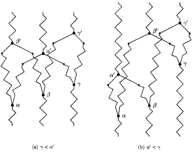
Consider P(l, 2; 3) as a subposet of B2 and take a minimal point, a. It is below

two maximal points, 61,62, so there is at least one path from a to bi and at least one path from a to 62- Choosing one path to b\ and one to b2, we can find the

(a) 7 < a ' (b) cl < 7

Figure 2.3: P ( l , 2; 3) with branching and connection points

branching points a, ß, 7 and the connection points a', ß', 7', so that a < ß < 7 and

a' < ß' < 7'. Each path contains both a branching point and a connection point, and since each connection point is contained in two paths, it must be greater than (at least) two branching points. In particular, a' must be greater than a and ß. Similarly, each branching point is less than (at least) two connection points, so 7

must be less than ß' and 7'. So, we have the inequalities ß < a' and 7 < ß', which gives the order a < ß < 7, a! < ß' < 7'. It is not possible to order 7 and a'. An example of the branching and connection points for the two cases 7 < a' and

a' < 7 are shown in Figure 2.3. Note that in Fig. 2.3(a) a' can be above any pair of branching points, whereas in Fig. 2.3(b) a' has to be above a and ß.

For a particular copy of P(l, 2; 3 ) ^ in B2 we have к copies of P ( l , 2; 3) so we can

sequences a, /3,7 of branching points and sequences ac', ß', V of connection points, where subscript i denotes the points in copy %. We have the order a* < Д < 7;, a[ <

ß[ < 7- for each г, as before. Call the points cti,ßi, 7i, г-branching points, and the points a'^ßl, 7-, г-connection points.

Ideally, we would aim to separate the copies of P(l,2;3) to analyse them indi-vidually (for example by assuming 7- < аг+1). Unfortunately this is not possible so

we have more cases to consider.

Since P(l, 2; 3 ) ^ is formed by identifying maximal points in copy г of P(l, 2; 3) to minimal points in copy г + l , we have that each (z+l)-branching point ai +i < /?i+1 <

7i+i is above (and therefore greater than) a distinct г-connection point ot[ < ß[ < 7г'.

This immediately gives the inequalities ai+x > a\ and 7. < 7i + 1. Looking at ßi+i,

either it is above ß[ or 7- which implies ßi+i > ß[, or it is above a- in which case is not above a[ and so must be above ß[ or 7-. But this implies A+i > «г+i > ß[. To summarise, we have

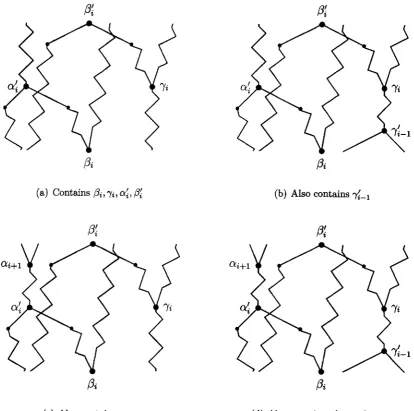
which is all we can deduce about the order of branching and connection points. Suppose we have a P ( l , 2 ; 3 ) ^ in B2[r,n]. We partition [r, n] into sets of two

types (plus two 'end' sets). A set of Type I is of the form [Д, /3-] and a set of Type II of the form [ßl+l, ßi+1-l]. The к sets of Type I and к-1 sets of Type II and the 'end'

sets [r, ß\ — 1] and [ß'k + 1, n] form the partition of [r, n]. We investigate which parts

can contain the branching and connection points. Clearly, ßi and ß[ are contained in the Type I sets. From (2.28) we have that 7 a [ <E [ßh /ЭД (г = 1 , . . . , к). Also, (2.28)

and (2.29) give the inequalities ß^ < аг < ßt and ß[ < 7- < ß'i+1 which implies that

a, e [A-i.A'-iM/^j + l . A - l ] (i = 2,...,k) and 7^ € [^ + l,/?i + 1-l]U[/3i + 1,^+ 1]

(г = 1 , . . . , к - 1). The end cases аг £ [r,ßi - 1] and G [ß'k + 1, n] are obvious.

So, looking at a Type I set [Д, /?•], it contains ßh 7г, a- and ß[ and possibly 7г'_! and OLi < ßi < < ßi < ii - for г = 1 , . . . , /г

ai +i>Q!- 7 i + i > 7 i for г = ! , . . . , * ; - 1

(2.28)

2 . 3 . A POSET NOT CONTAINED IN B2

ß'i

(a) Contains ß[ (b) Also contains

®i+1 «i+i