TMAS-TRIO MEASURE ASSESMENT SCHEME FOR
EFFICIENT ROUTING IN WIRELESS SENSOR NETWORKS
NAVANEETHAN.C#1, MUTYALA V.S.RATHNA KUMARI#2, THAMARAI SELVI.V#3, N.D.VIKRAM#4
#1
Assistant Professor(Senior), SITE School, VIT University, vellore,TamilNadu-632014
#2, #3, #4 M.Tech Software Technology, SITE School, V.I.T University ,vellore,TamilNadu-632014
E-mail: [email protected], [email protected], [email protected],
ABSTRACT
Wireless sensor networks have become one of the buzzwords in the field of networks. The challenging issue in wireless sensor networks is to design energy efficient routing in wireless sensor networks which is mainly focuses on increasing the network lifetime that emphasizes on main aspects namely residual energy, link condition, network lifetime. We introduced an appealing mechanism that supports for energy efficient
routing titled as”Trio Measure Assessment Scheme for Efficient Routing in Wireless Sensor Networks”. In
TMAS algorithm prioritized transmission count (PTX) is used for calculating node status and link quality in addition to this we will balance the load for enhancing the network life time. The main intention to introduce the scheme of load balancing is that sensor nodes that are closer to sink carries more inter-cluster traffic and hence deplete their energy faster than far away sensor nodes, So, by assessing the node status and link quality and load balancing we will get maximum results for efficient routing which will increase the network life time . Our Simulation results on TMAS prove that it outperforms the network lifetime and efficiently maintains the link quality among the clusters.
Keywords: TMAS,PTX ,Node Status, Link Quality, Network Lifetime, Inter-Cluster Traffic.
1. INTRODUCTION
Wireless sensor networks have become a
one of the solution media for wide range of applications including disaster management, security surveillance [1], agriculture, and in military. In general wireless sensor networks consists of tiny autonomous devices called sensor
nodes which aims at computing and
communication [2]. The main aspect of sensor nodes that should be emphasized during operations is its battery lifetime, as charging the battery for sensor nodes is an hectic task. So, it has become a challenging task to design an energy efficient [18] routing scheme for prolonging network lifetime where large amount energy is exhausted [3] during routing.
Clustering[3],[4],[5] is one of the effective techniques which results in the conservation of energy in the sensor nodes while routing, and it is consistent when compared to tree based and chain based routing[6] techniques, as they are cumbersome and doesn’t results an better outcome. The main challenge in the clustering technique is selection of the cluster
head nodes in multiple clusters and providing communication among those multiple clusters through the gateways. We will adapt the passive clustering [7] technique where each node has different states based on the state of information piggybacked in the received packet it changes its state. There are five external states to represent node’s role in a cluster. The external states include initial (IN), ordinary (OD), cluster head (CH), gateway (GW), and distributed gateway (D_GW)[7]. The PC technique also introduces two states, cluster head ready (CH_R) and gateway ready (GW_R), to represent the tentative role of a node. By this technique we can effectively diminish the communication overhead. Basically cluster heads consume more battery power. If the cluster head with a poor link quality and exhaust its battery power the routing path may be destroyed. Which results in, additional retransmissions that leads to energy consumption.
In most of the existing clustering techniques[8][9][10][11], cluster head selection is based on the residual energy[3],
degree of connectivity[15][16], node
adapt multi-hop communication to relay data sink as they cannot support long range communication. So the sensor nodes that are closer to sink carries more inter cluster traffic and hence deplete their energy faster than far away sensor nodes. This study motivates to develop TMAS algorithm that mainly intends to develop a mechanism for selecting the cluster head based on the prioritized transmission count (PTX).Once we select the cluster head and gateway. The gateways will manage sensor nodes under its cluster. We will balance the load[l] of the cluster by calculating the communication energy from the gateway node to all other sensor nodes within that cluster. Hence the overall traffic load of the sensor nodes can be better distributed so that there will be increase in network lifetime.
2. OBJECTIVE OF WORK
This section mainly describes the prioritized transmission count and the procedure for calculating the priority and load balancing in the proposed TMAS algorithm.
2.1 Network Model
We will consider an undirected graph G=(V,E),where V is the set of nodes and E subset of V ×V is the links between two sensor nodes.
Let e(i,j)єE denotes the link between two nodes si
and sj. In order to report the sensing data by the
sink it will periodically sends query messages to nodes. The report must satisfy the quality of sink expectation. That is, the reporting frequency must exceed a pre-defined threshold (Nreq).This threshold is conceded in query messages from the
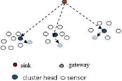
sink. The figure(1) describes about the basic
network architecture in wireless sensor
networks(WSN).In WSN for every cluster there will be a cluster head and gateways will provide communication among clusters.
Fig 1 Represents the location of sensor nodes in network area
2.2 Prioritized Transmission Count
Basic random selection of CH and GW nodes in the clustering technique doesn’t results in efficient outcome. Even selecting the cluster head based on the node id is not an proper approach because the sensor node having greater node id may not have better battery and lifetime which result in poor link quality[8] .So, in order to avoid this we will select the cluster head based on the priority. As we are calculating with respect to the neighboring node then there would be a persistent transmission. We can derive the PTX of CH and GW candidate by considering transit power, residual energy and link quality. A large PTX value indicates high probability of becoming CH or GW node. Because link reliability and data/message delivery ratio mainly depends on channel condition as, the channel condition varies with time in wireless links.
While calculating prioritized transmission
count(PTX) we have to evaluate the link
quality(LQ(i,j)) for node si to sj by making use of
forward delivery ratio(pf) and backward delivery
ratio(pb) from node si to sj. LQ(i,j) be the link
quality from the edge e(i,j).
LQ(i,j) = (1)
Here, each and every node periodically calculates
forward delivery ratio and backward delivery ratio and distance to its neighbors to assess the link quality by broadcasting messages .Then the node si derives the priority whenever it receives
report messages from its neighbors, we calculate priority by using (2).
Let PR(i,j) denote the prioritized transmission count of e(i,j) and the priority of candidate si, respectively
PR(i,j) = (2)
where Erem is the remaining energy of si, d(i,j) is the distance between si and sj , and Etx(k,d(i,j)) is the energy consumption for si to transmit a k-bit message of a distance d(i,j).The model of radio hardware energy dissipation this study uses is the first order model, in which the transmit power includes the energy to run the radio electronics and the power amplifier [17]. Let Etxelec(k) and
Etxamp(k, dn(i,j)) respectively denote the energy
consumption of radio electronics and the power amplifier to transmit a k-bit message a distance
[image:2.612.96.292.573.703.2]We have,
Etx(k, d(i,j)) = Etxelec(k)+Etxamp(k, dn(i,j))
(3)
The first order model make use of both the free space and the multipath fading channel models [11].Free space model is preferred when the distance between transmitter and receiver is less
than predefined thresh hold limit d0.Otherwise
multipath model is adopted . Let Eele represents
the electronics energy which is related to digital coding, filteration and modulation techniques. Etx(k, d(i,j)) = k*Eele+k*ɛfs* d2(i,j) if d(i,j) < d0,
Etx(k, d(i,j)) = k * Eele+ k *ɛmp* d 4
(i,j). else (4)
Here, ɛfs and ɛmp represents the amplifier energy
which describes the acceptable bit error rate and distance between transmitter and receiver.
3. DESCRIPTION OF TMAS ALGORITHM
TMAS algorithm has two stages namely Clustering and Balancing. In the first stage i.e. Clustering stage includes Discovering as well as clustering. In this stage we will discover all the surrounding nodes of sink by sending HELLO messages. Later we will calculate priority for CH, GW candidates by using (2) and then in the clustering process, based on the results of priority it assess the CH or GW candidates. Once we found the cluster head and gateway node we will balance the load which is done at the second stage.
3.1 Clustering Process
Initially ,sink node will send the HELLO messages to all other nodes and based on the report messages further process will goes on .i.e.,
Calculating the PTX PR(i,j)of all the neighboring
nodes of CH_R and GW_R candidates. Assume that all the sensor nodes are having the same communication range and they are stationary. let STnbr represents the set of si’s neighboring nodes
and NSTnbr be the number of sensor nodes in that
set. We will divide STnbr into two subsets, Sg (i)
and Sl (i) based on the comparison between calculated PTX and Nreq. In such a way that the subset Sg (i) is having the elements with PTX greater than or equal to Nreq, and the elements in Sl (i) are having PTXs smaller than Nreq . If Sg (i) ≠ф, set PR(i) as the PTX of the node, which has the minimum PTX in Sg (i) otherwise, set PR(i) as the PTX of the node, which has the
maximum PTX in Sl(i).By the definition of PTX, a candidate derives a large PTX value if it connects to nodes with a higher quality or supports more transmission counts. It determines the candidates satisfying the report quality by
putting them into Ssat (i). If Sg (i) ≠ф , it
considers the minimum PTX of all PTXs as the priority of si. This is because the link having minimum PTX can effectively support the report quality. If none of the links are able to satisfy the
report quality (i.e., Sg (i) = ф ), this study selects
the link that can support as many message reports as possible. Thus, the maximum PTX of all PTXs in Sg(i) as the priority of si .To ensure that the high priority node to be as a CH or GW node, TMAS make use of random back off approach to
suspend the transmission of data packets. Let Tiw
be the waiting period of candidate node si . Then, Tiw can be obtained as
Tiw =TsѲ( ) (5)
where Ts is the time slot unit, and Ѳ (x) rounds
the value of x to its nearest integer. Algorithm mentioned below will clearly describes this first stage.
3.1.1 Algorithm Prioritization Prioritized Transmission Count
./*To be performed by CH_R or GW_R node, Si
*/
Input: Nreq, NSTnbrtotal no of nodes in STnbr
Calculate PR(i,j) where Sj Sjnbr
PR(i,j)=
Sg(i)
(INITIALIZING)
Sl(i)
for j=1 to NSTnbrthen
if PR ij Nreq then
Sg(i)Sg(i) {Sj};
else
Sl(i) Sl(i) {Sj};
if Sgt(i) then
else
PR(i,j)=max qij, Sj Sl(i);
ReturnPR(i,j);
3.1.2 Algorithm clustering
Cluster State Transition
/* The node Si should perform when it receives
report messages from node Sj */
Input: Sicur,Sjcur,in(j)
Switch Sicur do
CASE IN
in(i) in(j) if Sjcur=CH then
SicurGW_R;
Call procedure transition; Else
If Sjcur=GW then
SicurCH_R
Call procedure transition; CASE OD
If(Sjcur=CH) and (in(i) in(j)) then
SicurGW_R;
Call procedure transition; Else
SinewSicur;
Otherwise
STinewSTicur
3.1.3 Algorithm Transition
Calculate Si
Determine Tiw
Is new state determined 0
While Ti
w
does not expire do report message from Sk then
If receive a report message from Sk then
If in(i) in(k) then
If Skcur=GW_R then
Sinew OD
Else
SinewGW
Procedure load
Else if Skcur=GW then
If Si cur
CH_R then
SinewCH
Else
SinewD_GW
Is New state Determined 1;
If is new state Determined=0 then
SicurGW_R then
If receive no report message from CH
Neighbors during Ti
w
then
SinewGW
Procedure load
Else
SinewOD
Sinew Sicur
Return Sinew
3.2 Load Balancing
The main purpose of balancing the load is due to inter-cluster traffic among the sensor nodes that are closer to the sink; it causes depletion of the energy. Here we will calculate Processing load PGi of a gateway Gi i.e., load required to process the data received from its sensors and the corresponding energy consumed
for the processing. Let Costji be the
communication cost which is a function of communication energy dissipated in transferring and receiving r bits of data over the distance
dSj->Gi. The communication cost Costji is
calculated as follows.
Cost E=Etx+Erx = (αtx+
αampd2)*r +αr*r (6)
Where Etx be the energy to send r bits and Erx is
the energy consumed to receive r bits. Assuming a path loss of 1/d2 for traversing a distance d.
where Etx, Erx are energy dissipated in
transmitting and receiving units per bit, αamp is
energy dissipated in transmitter amplifier, r is the number of bits in the message and d is the distance, the message traverses.
Then, the communication energy CEGI of a
gateway Gi is calculated as the sum of the communication cost of all sensors within the cluster.
CEGI =
∑
=
n
j tji 1
cos (7)
where, n is number of sensor nodes in the cluster. We now define the load of a gateway Gi as the function of processing load PGi and the communication energy CEGi, i.e.,
LGi=⌡(CEGI, PGI ) (8)
Since, we assume that all the sensor nodes deployed in the network are same and produce data at the same rate, and then the processing load PGi is directly proportional to number of sensor nodes within the cluster. It means that, to balance the load of each gateway, we have to balance the number of nodes per gateway. In addition to this, we have to minimize the communication energy required per gateway. To keep the system close to the average load, we choose an objective function called Root Mean Cardinality (RMC) of the system. That is,
where, CGk is cardinality of gateway Gk; cardinality of gateway indicates number of sensor nodes currently assigned to gateway Gk. |G| is number of gateways and X is number of sensor nodes currently assigned to various gateways.
3.2.1Algorithm Load Balancing
Procedure Load:
/* Input GW node Sj
For Si=1 to Nreq
{
Calculate cost
Costji =Etx+Erx;
CEGi= ji
} PGi=Nreq
Load= (PGi, CEGi)
If(RMC= )≥load
Then GWicurGWi
Else procedure contention
/* Assign GWi GW_R
Call procedure load End;
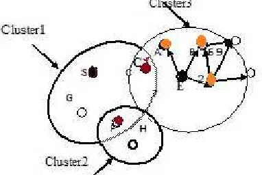
3.3 Diagramatic Representation Of TMAS Process
Fig(.a) represents the nodes within the communication range
Fig(b)represents that there are no neighboring CH nodes so node S will act as CH node.
fig(C) the nodes C, F, G becomes GW_R nodes as it receives message from CH node.
fig(d)As node C doesn’t have any GW neighbors it will become as a GW node and received Packet when its waiting time expires.To reduce the number of GW nodes it will calculate priority to select GW node. In addition to this we will Calculate the load , node F satisfies the criteria.
In fig(f) node E has higher priority so it act as CH. while node H will be CH and node E has higher Sj priority node E will be the CH node.
In fig.(g) nodes A,B,C will be in GW_R state as it Receives message from CH node E. Here, even Node B has highest priority but when we Calculate the CE it doesn’t satisfies Cluster2.
In fig. h node D satisfies the load so D is the GW node and A,B are in OD State and nodes I,J will be in CH_R state
5. SIMULATION RESULTS:
In the simulation we compared the
[image:6.612.83.523.48.735.2]passive clusterting (pc)technique and passive clustering technique–link quality and passive clustering–residual energy and proposed TMAS algorithm.Here,Fig(2) represents the comparision in terms of number of sensors nodes to the packet delivery ratio and Fig(3) represents comparision based on number of sensor nodes to the remaining energy
Table 1:Simulation Parameters.
Parameters Range of values
Network size 400 m × 400 m
Number of Sensor nodes
500
Communication range
100 m
Packet size 4000 bits
Initial battery power
4 Joule
Eele 50 nJ/bit
fs 10 pJ/bit/m2
mp 0.0013 pJ/bit/m4
Ts 100 ms
Nreq 5, 10
Simulation time 100 s
[image:6.612.91.282.275.403.2]Fig(3) Comparision On Different Passive Clustering Techniques Based On Remaining
Energy
5. PREVIOUS WORK
[1]Chun hung Richard Lin and Mario Gerla proposed an adaptive clustering algorithm for multimedia support. It is used to multi-hop
clustering architecture in mobile
network.[2].Arati Manjeshwar and Dharma P. Agrawal- Proposed a new energy efficient protocol, TEEN (Threshold sensitive Energy Efficient sensor Network protocol) for reactive networks. It is suited for time consuming critical applications and also it’s quite efficient for energy consumption. [3]. Wendi B. Heinzelman,et al., proposed a low-energy adaptive clustering hierarchy (LEACH). It is used to achieve good performance in terms of system life time and latency. It enables the self organization of larger networks. [4]. Stephanie Lmdsey, et al., in this paper they proposed a protocol called PEGASIS (Power-Efficient Gathering in Sensor Information Systems). It is an improvement over LEACH. [5]. Gaurav Gupta, et al., proposed an algorithm for wireless networks to sense all sensor nodes in the network. In which all the gateway nodes act as a cluster head and balances load.[6]. Dragos¸ Niculescu., et al., in this system they proposed positioning information for angle of arrival time for the orientation of nodes in the ad-hoc network. [7]. Ossama Younis et al.,proposed a protocol
called HEED (Hybrid Energy-Efficient
Distributed clustering) it will periodically selects the cluster heads according to the system residual energy for transmitting data to the neighboring nodes. [8]. Dali Wei, et al., in this to determine the residual energy and less power or energy consumption in the data sink level of the node of network.[9]Chia-Hung Tsai, et al., Proposed a systematical solution, which includes network formation, automatic address assignment and
light weight routing.[10] S.Banerjee
eteal.,proposed clustering scheme to
create a hierarchical control structure for multi-hop wireless networks[11]R.Eric et al., proposed
a sample opportunistic adaptive routing
protocol(SOAR) to explicitly support multiple simultaneous flows in wireless networks.[12]T. J. Kwon, et al., proposed novel clustering scheme, called Passive Clustering that can reduce the redundant rebroadcast effect in flooding,and demonstrated the efficiency of the proposed scheme in the AODV (Ad hoc, On demand Distance Vector) routing scheme.[13] Pratyay Kuila,et al, Proposed improved load balanced
clustering scheme for wireless sensor
networks[14] Zhixin Liu., et al., proposed DEECIC (Distributed Energy-Efficient Clustering
with Improved Coverage) algorithm and
additionally updates cluster heads according to
the joint information of nodes' residual
energydistribution[15] Sheng-Shih Wang et al. proposed an Energy and Link Efficient Clustering Technique for Reliable Routing in Wireless Sensor Networks.[16] C.P. Low.,et al., Proposed
an efficient -approximation algorithm for
the Load-Balanced Clustering
Problem (LBCP).[17] G. Gupta, et al., Proposed an algorithm to network these sensors in to well define clusters with less energy-constrained gateway nodes acting as cluster-heads, and balance load among these gateways[18] Ridha Soua and Pascale Minet introduced A Survey on Energy Efficient Techniques in Wireless Sensor Networks through which it provides a brief description of all the techniques involved in wireless sensor networks.
6. CONCLUSION
REFRENCES:
[1] F. Akyildiz, W. Su, Y.
Sankarasubramaniam, and E. Cayirci, “A
survey on sensor networks,” IEEE
Communications Magazine, vol. 40, no. 8,
pp102–114, Aug. 2002.
[2] J. Ford, “Telecommunications with MEMS
devices: An overview,” The 14th Annual
Meeting of the IEEE Lasers and Electro-Optics Society, vol. 2, no. 12, pp. 415–416,
Nov. 2001.
[3] O. Younis and S. Fahmy, “HEED: A hybrid,
energy-efficient, distributed clustering
approach for ad hoc sensor networks,” IEEE
Transactions on Mobile Computing, vol. 3,
no. 4, pp. 366–379, Oct. 2004
[4] G. Chen, C. Li, M. Ye, and J. Wu, “An
unequal cluster-based routing protocol in
wireless sensor networks,” Wireless
Networks, vol. 15, no. 2, pp a. 193–207,
Feb. 2009.
[5] Z. Xu, C. Long, C. Chen, and X. Guan,
“Hybrid clustering and routing strategy with low overhead for wireless sensor networks,” in Proceedings of the IEEE International
Conference on Communications (ICC), May
2010, pp. 1–5.
[6] C.-C. Chen and T.-K. Wu, “The survey of
data aggregation techniques in wireless sensor networks: Current approaches and future directions,” in Proc. Int. Conf. Digit.
Technol. Innov. Manage., 2006, pp. 1105–
1126
[7] T. J. Kwon and M. Gerla, “Efficient
flooding with passive clustering (PC) in ad hoc networks,” ACM SIGCOMM Computer
Communication Review, vol. 32, no. 1, pp.
44–56, Jan. 2002
[8] O. Younis and S. Fahmy, “HEED: A hybrid,
energy-efficient, distributed clustering
approach for ad hoc sensor networks,” IEEE
Transactions on Mobile Computing, vol. 3,
no. 4, pp. 366–379, Oct. 2004
[9] D. D. Couto, D. Aguayo, J. Bicket, and R.
Morris, “A high-throughput path metric for multi-hop wireless routing,” in Proceedings
of the ACM International Conference on
Mobile Computing and Networking
(MOBICOM), Sep. 2003, pp. 134–146
[10]M. Gerla and T.-C. Tsai, “Multicluster,
mobile, multimedia radio net-work,”
Wireless Netw., vol. 1, no. 3, pp. 255–265,
Aug. 1995
[11]T. S. Rappaport, Wireless Communications:
Principles and Practice. Prentice-Hall, 2002
[12]J. A. Torkestani and M. R. Meybodi,
“LLACA: An adaptive localized clustering algorithm for wireless ad hoc networks,”
Comput. Electr. Eng., vol. 37, no. 4, pp.
461–474, Jul. 2011.
[13]K. Lee, J. Lee, H. Lee, and Y. Shin, “A
density and distance based cluster head selection algorithm in sensor networks,” in
Proc. Int. Conf. Adv. Commun. Technol.,
Feb. 2010, pp. 162–165
[14]A.Tarachand, Vikas Kumar, Abhishek Raj,
Ashish Kumar, and Prasanta K. Jana,” An Energy Efficient Load Balancing Algorithm
for Cluster-Based Wireless Sensor
Networks
[15]M. Gerla and J.T.C. Tsai, “Multicluster,
mobile, multimedia radio network,”
ACM/Baltzer, Journal of Wireless
Networks,Vol.No. 1, pp. 255–265. 1995
[16]A.K. Parekh, “Selecting routers in ad-hoc
wireless networks,” In Proceedings of
SBT/IEEE International
Telecommunications Symposium, 1994
[17]W. B. Heinzelman, A. P. Chandrakasan, and
H. Balakrishnan, “An application-specific
protocol architecture for wireless
microsensor net-works,” IEEE Transactions
on Wireless Communications, vol. 1, no. 4,
660–670, Oct. 2002
[18]Ridha Soua and Pascale Minet “A Survey
on Energy Efficient Techniques in Wireless Sensor Networks”, IEEE Transactions on