Optimal Maintenance Modeling for Systems with Multiple Non Identical Units Using Extended DSSP Method

(1)

http://dx.doi.org/10.4236/ajor.2016.64027

How to cite this paper: Zhang, X.H. and Zeng, J.C. (2016) Optimal Maintenance Modeling for Systems with Multiple Non- Identical Units Using Extended DSSP Method. American Journal of Operations Research, 6, 275-295

http://dx.doi.org/10.4236/ajor.2016.64027

Optimal Maintenance Modeling for

Systems with Multiple Non-Identical Units

Using Extended DSSP Method

Xiaohong Zhang1,2_{, Jianchao Zeng}1,3*

1_{Division of Industrial and System Engineering, Taiyuan University of Science & Technology,}

Taiyuan, China

2_{School of Economics & Management, Taiyuan University of Science & Technology, Taiyuan, China} 3_{School of Computer Science and Control Engineering, North University of China, Taiyuan, China}

Received 9 April 2016; accepted 27 June 2016; published 30 June 2016

This work is licensed under the Creative Commons Attribution International License (CC BY). http://creativecommons.org/licenses/by/4.0/

Abstract

In the optimal maintenance modeling, all possible maintenance activities and their corresponding probabilities play a key role in modeling. For a system with multiple non-identical units, its main-tenance requirements are very complicated, and it is time-consuming, even omission may occur when enumerating them with various combinations of units and even with different maintenance actions for them. Deterioration state space partition (DSSP) method is an efficient approach to analyze all possible maintenance requirements at each maintenance decision point and deduce their corresponding probabilities for maintenance modeling of multi-unit systems. In this paper, an extended DSSP method is developed for systems with multiple non-identical units considering opportunistic, preventive and corrective maintenance activities for each unit. In this method, dif-ferent maintenance types are distinguished in each maintenance requirement. A new representa-tion of the possible maintenance requirements and their corresponding probabilities is derived according to the partition results based on the joint probability density function of the maintained system deterioration state. Furthermore, focusing on a two-unit system with a non-periodical in-spected condition-based opportunistic preventive-maintenance strategy; a long-term average cost model is established using the proposed method to determine its optimal maintenance parame-ters jointly, in which “hard failure” and non-negligible maintenance time are considered. Numeri-cal experiments indicate that the extended DSSP method is valid for opportunistic maintenance modeling of multi-unit systems.

(2)

Keywords

Extended Deterioration State Space Partition (DSSP), Condition-Based Opportunistic

Preventive-Maintenance, Hard Failure, Non-Negligible Maintenance Times, Multi-Unit Systems

1. Introduction

Preventive maintenance (PM) is a broad term that includes a set of activities to improve the overall reliability and availability of a system [1]. Many of today’s technological systems, such as aircrafts, nuclear power plants, military installations and advanced industrial and medical equipments, are comprised of multiple non-identical critical units. It involves high level of complexity in their maintenance and operation, due to interactions be-tween multiple units within a system. It is very important to design and implement appropriate and effective preventive maintenance for them. On one hand, these interactions must be taken into account in the maintenance decisions because of their strong influences. On the other hand, the interactions also offer the opportunity to group maintenance actions, which may save costs of system performance. Furthermore, improvements in ana-lytical techniques and the availability of fast computers have allowed more complex systems to be investigated [2]. Over the past decades, there has been a growing interest in the modeling and optimization of maintenance of systems consisting of multiple units. As can be seen in the related review papers [2]-[6].

According to the literature, opportunistic maintenance is an effective maintenance strategy for multi-unit sys-tems to collect units in a system that aims to reduce maintenance costs by grouping the maintenance activities of two or more units. Although the goal of opportunistic maintenance is to reduce maintenance costs, it may also impact plant availability. Therefore, the opportunistic maintenance policy was gradually studied in various mul-ti-unit systems maintenance modeling based on different maintenance strategies, such as age-based maintenance (ABM) strategy [7], failure-rate-tolerance-based maintenance (FBM) strategy [8] and condition-based mainten-ance (CBM) strategy [9].

In the optimization maintenance model, all possible maintenance requirements and their corresponding prob-abilities play an essential role in modeling. For a multi-unit system using opportunistic maintenance strategy, maintenance requirements can be dynamic groups with different combination of the system units, even with dif-ferent maintenance actions for these units. In order to formulate the decision problem of multi-unit systems with less mathematical difficulty, most of previous optimal preventive maintenance models for multi-unit systems were developed by means of some simple modeling method, such as Monte Carlo simulation techniques [10] [11]. And in these models, enumeration method is usually used to list all maintenance activities of the system. However, for a system with multiple units, simulation and enumeration method are more complicated and time-consuming, even omission may occur when enumerating its possible maintenance activities. Therefore, it needs to find a more efficient method to analyze the maintenance requirements and deduce their corresponding probabilities for these systems.

For a system composing n units, its deterioration space is an n-dimensional continuous state space. With the increasing of the number of units, the combination of the system states and its calculation for modeling grow exponentially. To deal with curse of dimensionality, many previous researched decomposes a multi-unit system into mutually influential single-unit systems and each single-unit system is formulated separately. Then, it de-veloped an approximation algorithm to obtain an acceptable maintenance policy for a multi-unit system, such as the studies by Wijnmalen and Hontelez [8], Jinqiu, H. and Z. Laibin [12] and Z. Zhang et al. [13]. However, if dependences between units are considered, the optimal maintenance decision on the whole system should de-pend on the deterioration state of the system rather than the deterioration state of individual units. That is to say, optimal maintenance of the individual unit cannot ensure the optimal maintenance of the whole system. There-fore, the decomposing method will injured much inaccuracy and cannot get an efficient maintenance policy since it can reduce the dimension of problem.

(3)

mainten-ance requirements at each maintenmainten-ance decision point are analyzed and their corresponding probabilities are deduced according to the partition results of the joint deterioration state of units. After then an explicit represen-tation of the srepresen-tationary law of the whole system deterioration is derived and its numerical solution is developed considering the dependences between units. Instead of giving an objective-specific optimization model (such as reliability, availability and cost rate or multi-objective), these studies only provide a generalized modeling me-thod for maintenance optimization of multi-unit systems. Also for simplification, the partition meme-thod in the re-cent study [15] only considered whether the unit should or not be maintained to model its deterioration state transition for a non-identical multi-unit system. However, for an objective-specific optimization model, it should not only distinguish which unit should be maintained, also which type of maintenance (opportunistic, preventive or corrective) should be performed on it due to their difference maintenance properties, such as cost and time. Therefore, a more detailed partition method should be studied to satisfy this modeling requirement.

In this paper, an extended DSSP method is presented for opportunistic maintenance modeling of general non-identical multi-unit systems by distinguishing the maintenance type of each unit. In the improved method, a more detailed partition is analyzed and new representation of the possible maintenance groups and their corres-ponding probabilities are derived based on it. Furthermore, in order to show the implementing process of the developed method, a non-periodical inspected condition-based optimization maintenance model is developed for a two-unit system considering hard failure and the non-negligible maintenance times. Using the proposed me-thod, a stochastic model for the long-term average cost per unit time is developed based on semi-regenerative process theory to determine the optimal inspection interval and control limits of units jointly.

The remaining sections are organized as follows. Section 2 describes the extended DSSP method. In Section 3, using the proposed method, a cost model is proposed to assess and optimize the performance of the maintenance policy for two-unit system. Section 4 presents a numerical example, where the analysis results show the imple-menting process of the developed method. Finally, Section 5 concludes the paper.

2. Extended DSSP Methods

The opportunistic maintenance policy was gradually used in various multi-unit systems maintenance modeling based on different maintenance strategies. In the previous proposed opportunistic maintenance strategy studies, a zone of “opportunistic maintenance” such as the age range

(

n N_i,

)

[7], the failure rate interval

(

L−u L,

)

[8] and the deterioration level interval ς( )j,ξk( )j

)

[9], is typically defined according to the control-limit policy to

determine which units should be opportunistically maintained given that a maintenance action on other unit is performed. For multi-unit systems with non-identical units, DSSP method is present in paper [15] to model the opportunistic maintenance of them. In the method, various maintenance actions are corresponded to various de-terioration state zones which are formed by splitting the dede-terioration state space of each unit with maintenance thresholds. For a system consisting of two or more units, the partition result of the system deterioration state is the crossover of the maintenance zone of every unit. More zones present more possible combinations of main-tenance actions. In this pare, all possible mainmain-tenance groups of general multi-unit systems with a known num-ber of non-identical units at each maintenance decision time and their corresponding probabilities are deduced using the presented approach. And further, a general representation of the stationary law of the system deteriora-tion and its numerical soludeteriora-tion is developed. Taking the common feature of the opportunistic maintenance policy into account, an extended DSSP method for opportunistic maintenance of multi-unit systems is proposed as be-low.

2.1. Characteristics of System

A multi-unit system with n non-identical units is considered, in which each unit deteriorates gradually. The gen-eral assumptions for the system are as follows:

1) The deterioration state of unit i i

(

=1, 2,,n

)

at time t can be described by a scalar random variable xt( )i

with initial state 0( ) 0

i

x = , which means the unit i is a new one. The unit i is considered failed as soon as its deterioration state exceeds a critical level D( )fi .

2) Let Xi

( )

t be the continuous stochastic process describing the deterioration process of unit i. On an infinite

discrete time grid tk

(

k∈N

)

, the stochastic process can be described as ( )

( )

N

i k

k∈

(4)

3) The increment of deterioration state of unit _{( )} _{( )} _{( )} i between two consecutive time units (i.e., between tk−1 and tk),

1

i i i k k k

x x x₋

∆ = − , is supposed to be nonnegative, stationary, and statistically independent, which follows the same distribution and the probability density function is fi

( )

x . Consequently, the distribution of the

incre-ments during n units of time is fi( )n

( )

x , where

( )n

_{( )}

i

f x is the nth convolution of fi

( )

x .

4) The global system deterioration evolution is modeled by the n-dimensional continuous stochastic process

( )

t =

(

1

( )

t ,, n

( )

t

)

X X X . The deterioration state of the system at time t can be described by n-dimensional

random variable

(

xt( )1,,xt( )n

)

and it be simplified as

(

x1,,xn

)

in the following.

The maintenance strategy is based on a control limit policy (CLP), which combines condition-based preven-tive, opportunistic and corrective maintenance. For each unit i i

(

=1, 2,,n

)

, the thresholds D( )pi and

( )i o

D

are defined for preventive maintenance and opportunistic maintenance respectively. It is generally assumed that

( ) ( ) ( )

0≤Doi ≤Dpi ≤Dfi . The detailed strategies are as follows:

1) Each unit is inspected non-periodically at discrete times tk

(

k∈N

)

, where k is the number of inspection and

k

τ is the interval of the kth inspection. After each inspection, the exact maintenance activities are deter-mined according to the deterioration state at that time, which is denoted as xi.

2) If ( ) i ( ) i i p f

D ≤x <D , the unit i is maintained preventively.

3) If i ( )f i

x ≥D , an corrective maintenance is performed on the unit i.

4) At each maintenance decision point, if a maintenance is performed on a unit i, for another unit j j

(

≠i

)

, if its deterioration state satisfies ( ) j ( )

j j o p

D ≤x <D , it is maintained opportunistically together with unit i. 5) Otherwise, the units are left as they are.

After maintenance, the maintained unit can be restored to “as good as new” state.

2.2. The Extended DSSP Method

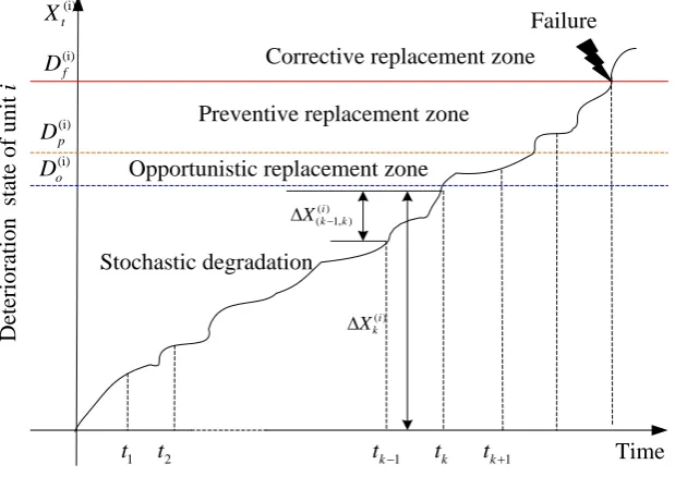
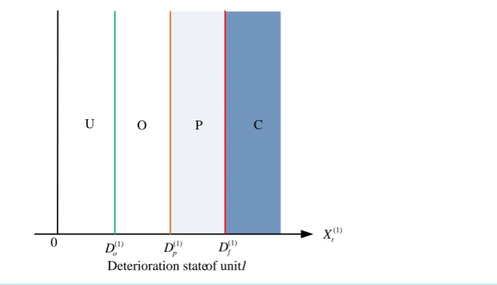
[image:4.595.160.470.485.704.2]

According to the defined strategy, Figure 1 illustrates the deterioration evolution of a single unit system. In this figure, the three maintenance thresholds of each unit split its deterioration state space into four zones: operating zone (U), opportunistic maintenance zone (O), preventive maintenance zone (P) and corrective maintenance zone (C). Each zone presents one maintenance action. Each zone presents one maintenance action. Therefore, the partition result of the deterioration state space of a single-unit system can be simplified asFigure 2 with distinguishing different maintenance types.

Figure 1. Deterioration model of the ith unit.

(i)

o

D (i)

p

D (i)

f

D

Time

Deterioration

state of unit

i

(i)

t

X

1

t t2 tk−1 tk tk+1

Corrective replacement zone

Preventive replacement zone

Opportunistic replacement zone

Stochastic degradation

Failure

( ) ( 1, )

i

k k

X − ∆

( )i k X

(5)

[image:5.595.176.535.79.285.2]

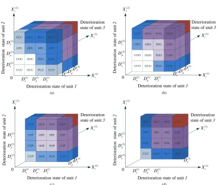
Figure 2. Deterioration state space partition of single-unit systems. For a system consisting of two or more units, the partition result of the system deterioration state is the cros-sover of the maintenance zone of every unit. Each zone presents a possible combination of maintenance actions of all units. The deterioration state space partition with all possible maintenance requirements in two-unit sys-tems and three-unit syssys-tems are depicted inFigure 3and Figure 4. InFigure 4, the partition result is divided into four subparts in accordance with four different maintenance requirements of the third unit: no maintenance (Figure 4(a)), opportunistic maintenance (Figure 4(b)), preventive maintenance (Figure 4(c)) and corrective maintenance (Figure 4(d)). In these figures, each deterioration state space region is named by a maintenance ac-tivity list which represents the maintenance requirement for each unit respectively.

For a multi-unit systems with n non-identical units, its possible maintenance requirement can be expressed as a maintenance activity list A A1 2An, where Ai denotes the maintenance activity for unit i and it have four

possible scenarios: U, O, P and C. Therefore, there are 4n possible maintenance requirements for a n-unit sys-tem corresponding with 4n deterioration state space regions. It’s easy to find that the possible maintenance re-quirement groups of n-unit system can be derived from the possible maintenance requirements of n − 1 units system by embedding its partition result to four possible scenarios: U, O, P and C of unit n. These possible maintenance activity lists are A A1 2A Un−1 , A A1 2A On−1 , A A1 2A Pn−1 and A A1 2A Cn−1 .

2.3. Maintenance Probability

Suppose π_n

(

x₁,,x_n

)

be the joint probability density function of the system deterioration state

(

x₁,,x_n

)

for a maintained multi-unit system with n non-identical units. Let PA An_{1 2}A_n denote the probability of the

main-tenance requirement A A1 2An. For a single-unit system, according to the partition in Figure 2, its

probabili-ties of all possible maintenance requirements can be deduced by the integrating the probability density function of the deterioration state, π₁

( )

x₁ , in its corresponding deterioration region, and the expressions can be ex-pressed as Equations (1)-(4).

( )

( )1

( )

1

U 1 ₀ 1 1 d1

o

D

P x =

∫

π x x (1)

( )

( )1

1 1

O 1 1 1 d 1

p o D D

P x =

∫

π x x (2)

( )

( )1

1

P 1 1 1 d 1

f p

D D

P x =

∫

π x x (3)

( )

( )1

( )

1

C 1 1 1 d1

f

D

P x =

∫

∞ π x x (4) The expressions of the probabilities of all possible maintenance requirements in two-unit systems also can be

Deterioration state of unit 1

(1) o

D

(1) t

X

(1) p

D D(1)f

0

(6)

[image:6.595.91.534.304.680.2]

Figure 3. Deterioration state space partition of two-unit systems.

(a) (b)

(c) (d)

Figure 4. Deterioration state space partition of three-unit systems. (a) The third unit needs no maintenance; (b) The third unit needs opportunistic maintenance; (c) The third unit needs preventive maintenance; (d) The third unit needs corrective main-tenance. Deterioration state of unit 2 (2) t X

Deterioration state of uint 1 (1) o D (1) t X (1) p D (1) f D (2) o D (2) p D (2) f D 0 UU OU UO OO PU CU PO CO OP PP UP CP

UC OC PC CC

Deterioration state of unit 1

(1) o D (1) t X (1) p D (1) f D 0

Deterioration state

of unit 2 (2) t X (2) o D (2) p D (2) f D (3) t X Deterioration state of unit 3

(3) o D (3) p D (3) f D PPC PPC PCC PPP PPP PPC PPC PCC PPP PPC PPC PCC PCC PPP PPC PPC PCC

O PPP PPC

PPP PPP PPC

PPC PPC PCC

UUU OUU PUU CUU

UOU OOU POU COU

UPU OPU PPU CPU

UCU OCU PCU CCU

Deterioration state of unit 1 (1) o D (1) t X (1) p D (1) f D 0

Deterioration state

(3) o D (3) p D (3) f D PPC PPC PCC PPP PPP PPC PPC PCC PPP PPC PPC PCC PCC PPP PPC PPC PCC UUO UOO UPO UCO

OUO PUO CUO

OOO POO COO

OPO PPO CPO

OCO PCO CCO

Deterioration state

(3) p D (3) f D PPC PPC PCC PPC PCC PPC PCC PCC UUP UOP UPP UCP

OUP PUP CUP

OOP OPP OCP POP COP PPP CPP PCP CCP

Deterioration state

(3) f D UUC UOC UPC UCC

OUC PUC CUC

(7)

presented by integrating the joint probability density function of the system deterioration state, π2

(

x x1, 2

)

, in

its corresponding deterioration state space region according to the partition inFigure 3. All the probabilities of maintenance activities for a two-unit system are as shown in Equations (5)-(20).

(

)

( )2 ( )1

(

)

2

UU 1, 2 ₀ ₀ 2 1, 2 d d1 2

o o

D D

P x x =

∫ ∫

π x x x x (5)

(

)

( ) ( )

(

)

( )2 1

2 2

UO 1, 2 ₀ 2 1, 2 d d1 2

p o

o

D D

D

P x x =

∫ ∫

π x x x x (6)

(

)

( ) ( )

(

)

( )2 1

2

UP 1, 2 ₀ 2 1, 2 d d1 2

o f p

D D D

P x x =

∫ ∫

π x x x x (7)

(

)

( ) ( )

(

)

1

2

UC 1, 2 ₀ 2 1, 2 d d1 2

o f

D D

P x x =

∫ ∫

∞ π x x x x (8)

(

)

( )

(

)

( ) ( )2 1

1 2

OU 1, 2 ₀ 2 1, 2 d d1 2

o p

o

D D

D

P x x =

∫ ∫

π x x x x (9)

(

)

( )

(

)

( ) ( )

( )2 1

2 1

2

OO 1, 2 2 1, 2 d d1 2

p P

o o

D D

P x x =

∫ ∫

π x x x x (10)

(

)

( )

(

)

( ) ( )

( )2 1

2 1

2

OP 1, 2 2 1, 2 d d1 2

P f

p o

D D D D

P x x =

∫ ∫

π x x x x (11)

(

)

( )

(

)

( ) ( ) 1 2 1 2

OC 1, 2 2 1, 2 d d1 2

P o f

D D D

P x x =

∫ ∫

∞ π x x x x (12)

(

)

( )

(

)

( ) ( )2 1

1

2

PU 1, 2 ₀ 2 1, 2 d d1 2

o f

p

D D D

P x x =

∫ ∫

π x x x x (13)

(

)

( )

(

)

( ) ( )

( )2 1

2 1

2

PO 1, 2 2 1, 2 d d1 2

p f

o p

D D D D

P x x =

∫ ∫

π x x x x (14)

(

)

( )

(

)

( ) ( )

( )2 1

2 1

2

PP 1, 2 2 1, 2 d d1 2

f f

p p

D D D D

P x x =

∫ ∫

π x x x x (15)

(

)

( )

(

)

( ) ( ) 1 2 1 2

PC 1, 2 2 1, 2 d d1 2

f p f

D D D

P x x =

∫ ∫

∞ π x x x x (16)

(

)

( )

(

)

( )2

1

2

CU 1, 2 ₀ 2 1, 2 d d1 2

o f

D D

P x x =

∫ ∫

∞ π x x x x (17)

(

)

( ) ( )

(

)

( )2

1 2

2

CO 1, 2 2 1, 2 d d1 2

p

o f

D D D

P x x =

∫ ∫

∞ π x x x x (18)

(

)

( ) ( )

(

)

( )2

1 2

2

CP 1, 2 2 1, 2 d d1 2

f

p f

D D D

P x x =

∫ ∫

∞ π x x x x (19)

(

)

( )2 ( )1

(

)

2

OC 1, 2 2 1, 2 d d1 2

f f

D D

P x x =

∫ ∫

∞ ∞ π x x x x (20) It is not difficult to induce that, for a multi-unit system with n non-identical units, the partitions of the deteri-oration space of the n units system can be constructed by embedding the partitions of the n−1 units system into the maintenance zones of the new unit. It can be known from Figure 2, there are four maintenance zones for the nth unit, operating zone (U), opportunistic maintenance zone (O), preventive maintenance zone (P) and

corrective maintenance zone (C), and their coverage regions are _0,D_o( )n

)

, _D_o( )n ,D( )_pn

)

, _D( )_pn ,D( )_fn

)

and

( )

)

, n f D  _∞

 respectively. Therefore, the probability of maintenance requirement A A1 2An can be formed by

(8)

Their probabilities can be expressed as Equations (21)-(24).

(

)

( )

(

)

1 2 1

1 1

U 1, 2, , 1, ₀ 1, 2, , 1, d1 d 1d n

o n

n n D n

A A A n n n n n n n

Q

P ₋ x x x x π x x x x x x x

−

− =

∫ ∫ ∫

− −





    (21)

(

)

( )

(

)

1 2 1

1 1

O 1, 2, , 1, 1, 2, , 1, d 1 d 1d

n p n n

o n

n D n

A A A n n _D n n n n n

Q

−

− =

∫ ∫ ∫

− −





    (22)

(

)

( )

(

)

1 2 1

1 1

P 1, 2, , 1, 1, 2, , 1, d 1 d 1d

n f n n

p n

n D n

A A A n n _D n n n n n

Q

−

− =

∫ ∫ ∫

− −





    (23)

(

)

( )

(

)

1 2 1

1

C 1, 2, , 1, n 1, 2, , 1, d1 d 1d

n

f n

n n

A A A n n _D n n n n n Q

−

− ∞

− =

∫ ∫ ∫

− −





    (24)

where Qn−1 denotes the deterioration state space region for maintenance activity list A A1 2An−1.

A special case is that when there is no unit in the system need to be maintained, all the opportunistic main-tenance requirements will be lay aside for no opportunity is offered. That is, in all regions crossover by operat-ing zone (U) and opportunistic maintenance zone (O) of all units, there is no unit need maintenance. Let

( )

0

n

M denote the random event that there is no maintenance requirement in a multi-unit system with n

non-identical units, its probabilities can be expressed as:

( )

(

)

(

)

( ) ( )

( ) 1 1

1 2 1 1 2 1 1 1

0 , , , , 0 0 0 , , , , d d d

n n

p p p

n

D D D

n

n n n n n n n

M

P x x x x π x x x x x x x

−

− =

∫ ∫

∫

− −

    (25)

In a multi-unit system with n non-identical units, the number of the regions crossover by operating zone (U) and opportunistic maintenance zone (O) of all units is 2n, therefore, the really number of the possible mainten-ance requirement combinations is 4n−2n+1

Equation (1)to Equation (25) indicate that the evaluation of such criterion requires determination of the joint probability density function of the deterioration evolution of the maintained system π_n

(

x₁,,x_n

)(

n=1, 2,

)

. In our previous study [15], the general expression, numeric solution, experimental verification and analysis of

(

1, , n

)(

1, 2,

)

n x x n

π  =  have been introduced in detail. It will not be repeated in this paper.

3. Optimal Maintenance Modeling for Two-Unit Systems

In order to show the implementing process of the extended DSSP method, the optimization model of the main-tenance for two-unit systems is established using the proposed method in this section.

3.1. System Characteristics

A two-unit system is considered in which each unit follows the general assumptions presented in Section 2.1. In addition, a consideration of hard failure is added. That is, the failure of each unit can be found immediately without inspections as it results in a system shutdown, which is referred as a hard failure [16]. In more detail, if the deterioration state of the unit i satisfies i ( )f

i

x ≥D at the time of inspection, an immediate corrective main-tenance is performed on the failed unit [17]. If its deterioration state xi exceeds the critical level

( )i f

D before a planning inspection, the system will down by itself, an immediate corrective maintenance is performed on the failed unit and the inspection plan is rearranged according to the deterioration state after maintained.

The maintenance strategy for this system is also based on the control limit policy defined in Section 2.2. Fur-thermore, non-periodical inspection intervals and non-negligible maintenance times are considered. More addi-tional detailed assumptions are as follows:

1) Let Cins be the specific unit cost for an inspection of the whole system. It consists of two parts,

( )1

ins

C for unit 1 and Cins( )2 for unit 2. The inspection of a component is assumed as perfect and non-destructive, and

the inspection time is considered negligible.

2) For unit i i

(

=1, 2

)

, the maintenance cost incurred by corrective maintenance and preventive maintenance are constant values Cc( )i and

( )i p

(9)

pre-ventive maintenance are tc( )i and

( )i p

t respectively. It can be generally considered that C( )pi Cc( )i and

( )i ( )i p c

t t . When preventive maintenance or corrective maintenance is performed, the system is shutdown. The time elapsed by the system in shutdown state incurs a cost at a cost rate Cd.

3) It is assumed that the opportunistic maintenance of each unit incurs same cost and time as its preventive maintenance.

4) After each maintenance, a new inspection interval is rearranged.

Either a scheduled maintenance with periodic inspection and/or an unscheduled corrective maintenance for hard failure is considered as a system intervention. In addition to the specific unit cost as previously defined, each intervention performance on the system entails a set-up cost Cs, which is assumed to be independent of

the nature of operation and incurred only once when several maintenance operations are performed at the same time.

3.2. Evaluation of the Performance Criteria of the Proposed Policy

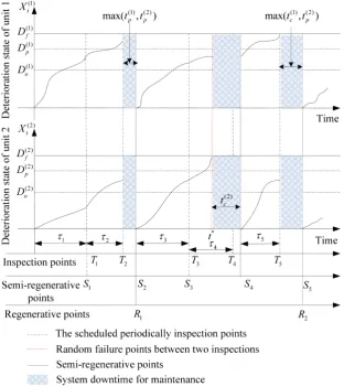
According to the defined strategy, an example deterioration and maintenance evolution of a two-unit system is illustrated in Figure 5.

[image:9.595.159.472.351.703.2]

In this figure, Tk

(

k∈N

)

are the scheduled inspection points. At the inspection time T1 and T3, no main-tenance is required because there are no mainmain-tenance opportunities even though the deterioration states of the units belong to their opportunistic maintenance zones, the next inspection date for the system is scheduled ac-cording to the deterioration state at that time respectively. At the inspection time T2, a preventive maintenance

(10)

is required for the unit 1. While the deterioration state of unit 2 belongs to its opportunistic maintenance zone, it is opportunistically maintained together. After a certain maintenance interval, the system is restored to a new state and a new inspection cycle begins. At time t* between the inspection times T3 and T4, the deterioration state of unit 2 exceeds its critical level, and immediately a corrective maintenance is incurred. At that time, the system is shut down for maintenance. After maintenance, the system is also restored to “as good as new” state and an inspection is scheduled. At the inspection time T5, a preventive maintenance is required for the unit 1. The deterioration state of unit 2 is greater than its opportunistic maintenance threshold and opportunistic main-tenance is required. It can be seen fromFigure 5, at times R1 and R2, all of the units in the system are main-tained and the system is restored to “as good as new” state. Thus, these points are denoted as regenerative points. However, at times S2, S4 and S5, parts of system units are maintained and restored to their new states. To-gether with inspection points S1 and S3, all these points are denoted as semi-regenerative points.

It’s easy to find that the length of a semi-regeneration cycle is varying stochastically. Let the stochastic varia-ble S be the length of a semi-regeneration cycle. It contains two time stochastic periods: 1) Uptime interval be-tween the last starting up time and the system failure time or the next periodical inspection time, denoted as S′, which varies stochastically with the stochastic failure and dynamic inspection interval. 2) Downtime for main-tenance, denoted as D, which varies stochastically with the maintenance activities for stochastically deteriora-tion.

A cost model is proposed to assess and optimize the performance of the proposed policy. According to re-newal theory, the average cost of an infinite time is defined a,

( )

expected cost on one semi-renewal cycle

(

_{( )}

( )

)

lim

expected length of a semi-renewal cycle

t

E C C t

CR t

t

S

E S →∞

= ≈ = (26)

where E S

( )

is the expectation of the time length of a semi-regeneration cycle. The term E C S

(

( )

)

denotes the expectation of the total cost of the semi-regeneration cycle.

In accordance with the characteristics of the system deterioration process and the maintenance strategies de-scribed above, the choices of the inspection interval and the opportunistic and preventive maintenance thre-sholds for each unit influences the performance of the proposed policy. If the inspection interval is too large, the probability of failure increases between two inspections, which results in increased maintenance costs. In con-trary, it is expensive to inspect the system too frequently. Similarly, the low opportunistic and preventive main-tenance thresholds result in frequent preventive mainmain-tenance and the remaining life of the deteriorated but still working unit cannot be fully exploited. Otherwise, the failure probability and the maintenance costs increase between two inspections. To minimize the total maintenance cost of the whole system, the optimization of the proposed policy can be defined as a constrained optimization problem, if the average cost can be represented as a function of these decision variables as following:

( )

(

( ) ( ) ( ) ( )

)

( ) ( )

(

)

( ) ( ) ( )

1 2 1 2

1 1

1 2

1 1 1

2 2 2

min min , , , ,

. . ,

k p p o o k k

k

o p f o p f

D D D D

s t m x x

CR

D D D

D t

D D

τ

τ − −

= Ψ

=

≤ ≤

≤ ≤ (27)

The unit i i

(

=1, 2

)

is considered failed as soon as its deterioration state exceeds its critical level D( )fi , and

the system is shutdown for the unit failure. Due to the characteristic of hard failure, the exact time of failure of unit i is unknown. Therefore, the kth stopping of the operation system can be two scenarios: 1) Pre-scheduled inspection, in which case the length of the kth uptime duration is Sk′ =τk. (2) System failure between two

in-spections, in which case the length of the kth uptime duration is S′ =k τkf

(

0<τfk <τk

)

. It should be explain that

if a failure occurs at time τkf with

(

0,

]

k

f k

τ ∈ τ . In order to facilitate the analysis, an infinite discrete time grid is adopted here, it is assumed that the exact time of failure of unit i can be set as any one integer value between

(

0,τ_k

]

. That is to say, it is assumed that that the exact failure time is at the integer discrete time if it occurs in a time unit. Let

(

| i;

)

k f k i

(11)

after the last semi-regeneration point given that the revealed deterioration state equal yi′ and the next

inspec-tion was scheduled τk time units later (Castanier, Grall, & Bérenguer, 2005). This probability can be

ex-pressed as,

(

)

(

( )

)

0 _if | i ; f k f k f k k k f k _i

f k i f i i i f D H y y τ τ τ

τ ′τ  _τ >_τ

≤ ′

 = 

−

 (28)

The expected uptime duration in a semi-regeneration cycle is expressed as:

( )

1

(

)

(

)

1 k

k f

k k

f f k k

S P S P S

E

τ

τ τ τ τ

−

=

′ =

∑

′= + ′= (29)

Using tf as the exact failure time of the system, Equation (33) can be obtained.

(

) (

)

(

) (

)

(

)

(

)

1 1 1 1

k k k

f f f f k k f f f f

k k

f f f f

P S P t

P t P t

τ τ τ

τ τ

′ = = − < ≤

= ≤ > −

 

= ≤ _ − ≤ − _ (30)

The failure of the system can be triggered by failure of unit 1 and/or unit 2, therefore,

(

)

2

(

) (

)

1 2

1

,

i

f f f f

i

P t r P t r P t r t r

=

= =

∑

= − = = (31)

In Equation (31), P t

(

if =r

)

(

i=1, 2

)

consider the scenario that each unit in failure state separately,

(

1 2

)

,

f f

P t =r t =r takes into account the scenario that both units are simultaneously in failure state. These prob-

abilities can be evaluated by analysis of all the scenarios leading to failure. The failure of unit i may occur under two conditions. If unit i was maintained at its previous semi-regenerative point, then yi′ =0. If unit i was not maintained at its previous semi-regenerative point, then yi′ =yi <D( )pi and

( )i

₍

₎

j p

y <D i≠ j or yi′ = <yi Do( )i

and yj≥D( )pi

(

i≠ j

)

. Therefore, the probability of the unit i being in failure state is expressed as Equation (32),

and the probability of both units being simultaneously in failure state is expressed as Equation (33).

(

)

( ) ( )

(

)

( )

(

)

( ) ( ) ( )

(

)

(

)

( ) ( )

(

)

( )

(

) (

)

( )

(

) (

)

( ) ( ) 2 1

2 1 2 1 2 1 2 2 1 2 1 2 1 2

2 1 2 2 1 2

0 0

2 1 2

0 0

, d d , d d | 0,

, d d | 0, , | , d d

, | , d d

p p

o o o o

j i o o i j p p i j p p D D i

f _D _D _D _D i k

D D

i j i k i i k j i

D D

i i k j i

P t r y y y y y y y y H r

y y y y H r y y H r y y y

y y H r y y y

π π τ

π τ π τ

π τ ∞ ∞ ∞ ∞   = =_ − _     +_ _ +   +

∫ ∫

(32)

(

)

( ) ( )

(

)

( )

(

)

( ) ( ) ( )

(

) (

)

(

)

( )

(

)

(

)

(

)

( ) ( )

(

)

(

)

(

) (

)

2 1

2 1 2 1

2

(1)

1

2

1 2

2 1 2 1 2 2 1 2 1 2 1 2

2 1 2 1 2 2 2 1

0

2 1 2 2 1 1 1 2

0

2 1 2 1 1

, , d d , d d | 0, | 0,

, d | , d | 0,

, | ,

p p

o o o o

o p

D D

f f _D _D _D _D k k

D k k D D k k D k

P t r t r y y y y y y y y H r H r

y y y H r y y H r

y y y H r y y H r

y y H r y H

π π τ τ

π τ τ

π τ ∞ ∞ ∞ ∞   = = =_ − _     + _ _   + _ _ +

∫ ∫

(

)

( ) ( )1 2

2 2 2 1

0 0 | , d d

p p

D D

k

r y τ y y

∫ ∫

(33)

If the system has not failed between two inspections, the operation of the system can be stopped by pre- scheduled inspection. Therefore, the probability of the length of the uptime duration is S′ =τk can be

(12)

(

)

1

(

)

1

k

k f

k

k P Sk f

P S

τ

τ − τ

=

′

= − =

′ =

_∑

(34)

If the operation of the system is stopped by pre-scheduled inspection, all units in the system are inspected and the maintenance activities are arranged according to the revealed states. Different maintenance groups incur dif-ferent probabilities and costs. According to partitions inFigure 3, the revealed system state can falls in 16 re-gions. Different cost will incurred for different regions with different probability which can be calculated ac-cording to to partitions inFigure 3, the revealed system state can falls in regions:

1) OO , UO , OU and UU , no maintenance is performed, only the system inspection cost Cins need to be

paid and no maintenance time is consumed. The probability of this occurrence is :

( )

(

)

(

)

( ) ( )2 1

2 2

1 2 2 1 2 1 2

0 , 0 0 , d d

p p

D D

M

P x x =

∫ ∫

π x x x x (35) 2) PU or UP , only unit 1 or unit 2 needs a preventive maintenance with probability PU

(

)

2 1, 2 P x x or

(

)

UP

2 1, 2

P x x . If the maintainable unit is i i

(

=1, 2

)

, the unavailable duration for maintenance is t( )pi and the

maintenance costs is Cins +Cs+Cp( )i +Cd ⋅t( )pi .

3) PO , OP and PP, due to the assumption that the opportunistic maintenance of each unit incurs same cost and time as its preventive maintenance, in these scenarios, the unavailable duration for maintenance is

( ) ( )

(

1 2

)

max tp ,tp and the maintenance costs can be expressed as

( )1 ( )2

(

( ) ( )1 2

)

max ,

ins s p p d p p

C +C +C +C +C ⋅ t t .

The probability is POP2

(

x x1, 2

)

+PPO2

(

x x1, 2

)

+PPP2

(

x x1, 2

)

.

4) CU or UC , only unit 1 or unit 2 needs a corrective maintenance with probability CU

(

)

2 1, 2 P x x or

(

)

UC

2 1, 2

P x x . If the maintainable unit is i i

(

=1, 2

)

, the unavailable duration for maintenance is tc( )i and the

maintenance costs is Cins +Cs+Cc( )i +Cd ⋅tc( )i .

5) OC and PC , the unavailable duration for maintenance is max

(

t( ) ( )p1,tc2

)

and its maintenance costs can be

expressed as C_ins+C_s+C_p( )1 +C_c( )2 +C_d⋅max

(

t_p( ) ( )1,t_c2

)

. The probability of its occurrence is

(

)

(

)

2 2

OC 1, 2 PC 1, 2

P x x +P x x .

6) CO and CP , the unavailable duration for maintenance is max

(

tc( ) ( )1,tp2

)

and its maintenance costs can be

expressed as Cins+Cs+Cc( )1 +C( )p2 +Cd⋅max

(

tc( ) ( )1,tp2

)

. The probability of its occurrence is

(

)

(

)

2 2

CO 1, 2 CP 1, 2

P x x +P x x .

7) CC , the unavailable duration for maintenance is max

(

t_c( ) ( )1,t_c2

)

and the maintenance costs is

( )1 ( )2

(

( ) ( )1 2

)

max ,

ins s c c d c c

C +C +C +C +C ⋅ t t . The probability of its occurrence is PCC2

(

x x1, 2

)

.

If system failure occurs between two inspections, it contains two sub-scenarios:

1) If the system failure is triggered by failure of one unit i i

(

=1 or 2

)

. Its failure probability is

(

) (

1 , 2

)

k k k

i f f f

P S′=τ −P S′=τ S′=τ . A corrective maintenance is performed on unit i and an inspection is

per-formed on unit j j

(

≠i

)

.

a) If xj <Do( )j , the unit j will not be maintained, the unavailable duration only contains corrective maintaining

time for unit i, tc( )i , and the maintenance costs can be expressed as

( )j ( )i ( )i ins s c d c

C +C +C +C ⋅t . The probabil-ity of its occurrence is:

(

)

( ) ( )

2 1 2

0 , d d

j o

i f

D

i j D π x x x x

∞

(13)

b) If Do( )j ≤xj <D( )fj , the unit j will be preventively maintained simultaneously with unit i. Compared to the

previous sub-scenario, the unavailable duration is the maximum of the corrective maintaining time for unit i,

( )i c

t , and the preventive maintenance time for unit j, t( )pj , then the maintenance costs can be expressed as

( ) ( ) ( )

(

( ) ( )

)

max ,

j i j i j ins s c p d c p

C +C +C +C +C ⋅ t t . The probability of its occurrence is:

(

)

( ) ( )

( )

2 1, 2 d d

j f i j o f D i j D D π x x x x

∞

∫ ∫

(37)

2) If the system failure is triggered by failure of two units, its probability is P(S '₁ =τk_f,S '₂ =τk_f). At that time, the entire system will be correctively maintained simultaneously. The unavailable duration for maintenance

is max

(

tc( ) ( )1,tc2

)

and the maintenance costs is

( ) ( )

(

( ) ( )1 2

)

max ,

i j

s c c d c c

C +C +C +C ⋅ t t .

The expected total cost of a semi-regenerative cycle is concluded by Equation (38),

( )

(

)

(

)

{

( )

(

)

(

( ) ( )

)

(

)

( ) ( )

(

)

(

)

( ) ( )

(

( ) ( )

)

(

)

(

)

(

)

(

( ) ( )

)

₍

₎

2 1 2 2

1 2 PU 1 2

0 1

2 UP 1

1 1

2 2 1 2 1 2

2

PO 1 2 OP 1 2 PP 1 2 CU 1 2

1 1

max ,

1 , ,

,

, , , ,

k

k f

ins ins s p d p

ins s p d p ins s p p d k

f M

p p ins s c d c

S P S P x x P x x

P x x

P x x P x x

E C C C C C C t

C C C C t C C C C C t t

C C C C

P x x

C P x t x τ τ τ − =   =  − =  ⋅     + + + ⋅ + + + + ⋅ ⋅   + + + + ⋅ ⋅ _ + + + + ⋅ _ ⋅_ _+ + + + ⋅ ⋅ +

∑

( ) ( )

(

)

(

)

( ) ( )

(

( ) ( )

)

₍

₎

( ) ( )

(

( ) ( )

)

₍

₎

( ) ( )

(

( ) ( )

)

₍

₎

}

(

) (

)

2 2 1 2 1 2

1 2 1 2

1

2 2

UC 1 2 PC 1 2

2

CP 1 2

2

CC 1 2

1 2

1

2 1 2

max , max , max , , , , , , k k f

ins s c d c ins s p c d p c ins s c p d c p

ins

k k k

i f f f i j

s c c d c c

C C C t C C C C C t t

C C C C C t t

P x x P x x

P x x

P S P S S

τ

τ τ τ

≠ =   + + + ⋅ ⋅ _ + + + + ⋅ _⋅   +_ + + + + ⋅ _⋅   + + + + + +    + _ = − = =     ⋅ ⋅ 

∑

(

( ) ( ) ( )

)

₍

₎

( ) ( ) ( ) ( ) ( )

(

( ) ( )

)

(

)

( ) ( )

(

)

( )

(

)

(

( ) ( )

(

( ) ( )

)

}

1 1 2 0 1 2 1

2 1 2

2

1

, d d

, max , max , j o i f j f i j o f

j i i ins s c d c j i j i j

ins s c p d c

D i j D D i j D D k k f p

s c c d c

f c

C C C C t

C C C C C t t

C C C

x x x x

P S S C t t

π π τ τ − _∞ ∞  ⋅ _  + ⋅ _ + + + ⋅ ⋅ + +  + + + ⋅ + + = = ⋅ + ⋅

∑

∫ ∫

(38) Based on the above analysis, the expected unavailable duration for maintenance over a semi-regenerative cycle can be expressed as Equation (39).

( )

(

)

{

( )

₍

₎

( )

₍

₎

(

( ) ( )

)

(

)

(

)

(

)

( )

₍

₎

( )

₍

₎

( ) ( )

(

)

(

)

(

( ) ( )

)

₍

₎

(

( ) ( )

)

₍

₎

}

(

)

1 2 2

PU 1 2 UP 1 2

1

2 2

PO 1 2 OP 1 2 PP 1 2 1 2 UC 1 2

2 2 2

PC 1 2 CP

1 2 1 2

1 2

1 2 1 2 1 2

1 2 CC 1 2

max ,

max , max , max

1 , ,

, , , , ,

, , , ,

k

k f

p p p p

c c

p c c p c

k f C f c U k i

E D t t t t

t

P S P x x P x x

P x x P x x P x x P x x t P x

t t t t t t

x

P x x P x x P x x

P S P

τ τ τ τ − =     ⋅ + = − = ⋅ + + +     + + ⋅     ⋅ = + ⋅ + ⋅ ⋅ + ⋅ + ⋅ −

∑

(

)

( )

₍

₎

( ) ( ) ( ) ( )

(

)

( ) ( )

(

)

( )

(

)

(

( ) ( )

)

1

1 2 ₀ 1 2

1

1 2 1 2

1 2

m

, , d d

, d d ,

ax , max ,

j k o i f k f j f i j o f D k k

f f _D i j

i j

D _k _k

i j i c

i j

c p _D _D f f c c

t

t t

S S x x x x

x x x x P S S t t

τ

τ τ π

π τ τ

− _∞ ≠ = ∞  = = ⋅     + ⋅ _+ = = ⋅ _   _⋅  _   

∑ ∑

∫ ∫

(39)

(14)

of constraint variables. A genetic algorithm (GA) is chosen as an optimization method to solve the model be-cause it can deal with linear and nonlinear, constrained and non-constrained, as well as discrete, continuous, and hybrid search spaces.

4. Numerical Experiments

4.1. Experimental Results

A numerical example is presented herein to demonstrate the correctness and validation of the DSSP method. A gamma distribution is often used to characterize continuous wear processes with non-negative, stationary, and statistically independent increments starting from zero level [9] [17]. An advantage of the gamma distribution process is the existence of an explicit probability distribution function which permits feasible mathematical de-velopments [18]. Therefore, we assume that the deterioration increments of unit i, ∆xk( )i , follow the gamma

dis-tribution, Γ

(

α βi, i

)

. Its probability density function can be expressed as:

(

)

_{( )}

( )

1

0

1 | ,

d e

e , 0

, 0

i i

i

x i

i

i i

x i

i x x

f x x x

α

α β

α

α α

α β − −

∞ _{− −}

= ≥

Γ

Γ =

_∫

> (40)

A gamma wear process in continuous time z follows the gamma distribution Γ

(

zα β_i, _i

)

.

The kth inspection interval τk is defined as a function of the system deterioration state after the previous

maintenance decision,

(

1( )1, 2( )1

)

k k

m x − x − , where m

( )

⋅ is a decreasing function from 0 to T (Grall, Dieulle et al. 2002). In the numerical experiment, we define m x x

(

1, 2

) (

= −1 a x1 1−a x2 2

)

T as an experimental function to

ensure the maximum inspection interval is T. Therefore, determination of the optimal τk is to determine the

optimal value of the coefficients a1 and a2.

For two non-identical units, we suppose that: α =1 1, β =1 1.5, α =2 2, β =2 2, ( )1

4

f

D = , D( )f2 =5. When τ =k 3,

( )1 2.5

o

D = , Do( )2 =3.5,

( )1 3.5

p

D = , D( )p2 =4, and truscated data is defined as

( )1 6Df and

( )2

6Df instead of ∞, approximate numerical solution of π

(

x x1, 2

)

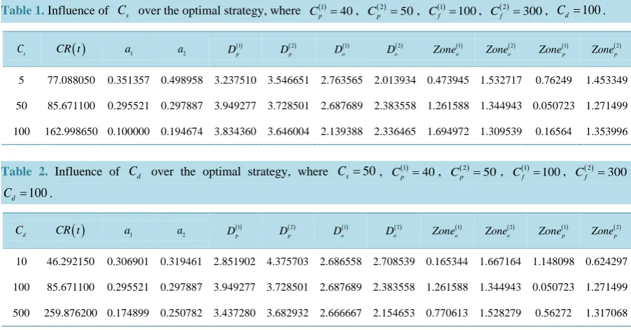
is shown inFigure 6.

We will verify the proposed deterioration state space partition method by making a decision table and per-forming sensitivity analysis of different parameters. Additionally suppose that C( )p1 =40,

( )2 50

p

[image:14.595.99.536.492.703.2]

C = , Cc( )1 =100,

Figure 6. Example of deterioration and maintenance evolution of a two-unit system.

0 5

10 15

20 25

0 5 10 15 20 25 300 0.005 0.01 0.015

Deterioration state of unit 1 Deterioration state of unit 2

S

tat

ionar

y

pr

obabi

lit

y

dens

it

y

f

unc

ti

(15)

( )2 300

c

C = , t( )p1 =0.5,

( )2 1

p

t = , tc( )1 =2,

( )2 4

c

t = , Cs=50, Cd =100,

( )1 2

ins

C = , Cins( )2 =3, then Cins=5,

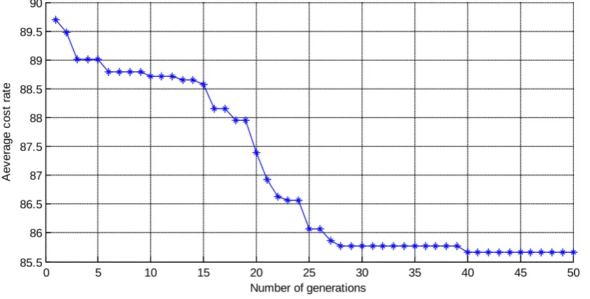
and T=10. The approximate optimal value of the expected costs per unit time is obtained using GA with parameters set as follows: population size is 20, maximum number of generations is 50, generation gap is 0.8, crossover rate is 0.8, and mutation rate is 0.2.Figure 7 shows an example of the evolution of the optimization process. The optimal values of the decision variables are α =1 0.295521, α =1 0.297887,

( )1

2.683018

p

D = ,

( )2

3.461388

p

D = , Do( )1 =1.003265,

( )2

2.920907

o

D = corresponding to the minimal cost rates

( )

85.671100

CR t = .

4.2. Sensitivity Analysis

From the definition of π₂

(

x x₁, ₂

)

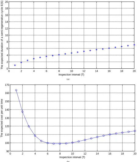
, we discover that adjustment of the length of the inspection cycle and oppor-tunistic and preventive maintenance thresholds can result in different stationary probability density functions. Further, it can influence the probabilities of all possible maintenance groups. In a specific maintenance optimi-zation model, it can obtain different specific target values for different choices. For facilitation, we analyze the effects of the inspection interval on the expected duration of a semi-regenerative cycle and the expected cost per unit time with a deterministic value T. Their relations are presented inFigure 8. We can observe from Figure 8(a)that E S

( )

increases with increasing inspection period T. However, its rate of growth reduced gradually and reached an asymptote at a certain time. Because the probability that random failure occurs in an inspection interval is lower when T is smaller, the expected duration of a semi-regenerative cycle approaches the length of the inspection period. When T becomes larger, the probability that a random failure occurs in an inspection in-terval increases. Then, the expected duration of a semi-regenerative cycle gradually closes to the natural failure period of the system. The results inFigure 8(b) indicate minimal values of expected costs per unit time with different values of T. It can be observed from the this figure that expected costs rate increase with increasing T

after their optimal values, due to the increase in the corrective maintenance costs and the probability that random failure occurs in an inspection interval. However, the growth curve of the expected cost rate becomes smooth when T becomes too large because the expected duration of a semi-regenerative cycle gradually closes to the natural failure period of the system.

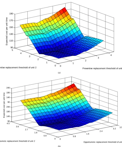
Next, we focus on the influence of the opportunistic and preventive maintenance thresholds of each unit over the optimal values. When T=5, Do( )i =Dp( )i

(

i=1, 2

)

, and

( )i p

D varies from 0 to D( )fi , the results inFigure

9(a) show minimal values of expected total costs with different preventive maintenance thresholds. When 5

T= , D( )p1 =3.5,

( )2 4.5

p

D = , and Do( )i varies from 0 to

( )i p

[image:15.595.105.527.489.703.2]

D , the results in Figure 9(b) show minimal

Figure 7. An example of optimization result of GA.

0 5 10 15 20 25 30 35 40 45 50

85.5 86 86.5 87 87.5 88 88.5 89 89.5 90

Number of generations

A

ev

er

age c

os

t r

at

(16)

(a)

[image:16.595.89.539.86.618.2]

(b)

Figure 8. Effects of inspection interval on the optimization objective. (a) On the expected duration of a semi-regenerative cycle; (b) On the expected cost per unit time.

values of expected total costs with different opportunistic maintenance thresholds. Figure 9 indicate that the cost rate is relatively small at smaller D( )pi and

( )i o

D due to the higher probability of preventive maintenance and lower probability of random failure, and combined with the fact that preventive maintenance costs are less than corrective maintenance costs. But if D( )pi and

( )i o

D is too small, frequent preventive maintenance also incurs high costs. With the increase in preventive maintenance thresholds, preventive maintenance zone

gradu-0 2 4 6 8 10 12 14 16 18 20

0 2 4 6 8 10 12 14 16 18 20

Inspection interval (T)

T

he ex

pec

ted dur

at

ion of

a s

em

i-regener