Sizing the Government

Munich Personal RePEc Archive

Sizing the Government

De Witte, Kristof and Moesen, Wim

University of Leuven

22 April 2009

Online at

https://mpra.ub.uni-muenchen.de/14785/

Sizing the government

Kristof De Witte

and

Wim Moesen

University of Leuven (KUL)

Naamsestraat 69

3000 Leuven, Belgium

[email protected]

www.econ.kuleuven.be/kristof.dewitte

April 22, 2009

Abstract

Is there such a thing as an optimal government size? We investigate by the

non-parametric Data Envelopment Analysis (DEA) the so-called ‘Armey curve’ which claims

an inverted U-shaped relationship between government size and economic performance.

The DEA scores are linked to control variables as initial per capita income, openness,

population density, urbanization, country size and family size. For 23 OECD-countries

we estimate the country speci…c e¢ciency scores, which reveal the extent to which a

country uses excess public resources to achieve the observed growth rate of GDP.

JEL Classi…cation: H10, H21, H31

Keywords: Data Envelopment Analysis, Government size, Public sector

perfor-mance, Armey-curve.

Introduction

During the second half of the last century, government involvement in OECD-countries

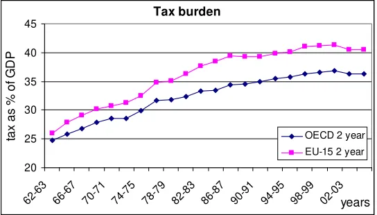
ex-panded rapidly. Whereas the size of the tax burden (i.e., the ratio of tax revenue to GDP)

was 24.7% in 1960, the tax burden reached an average of 36.3% in 2003. Many theories

for the growth of government have been o¤ered. Wagner’s law (1877) states that the

de-mand for governmental services has an income elasticity in excess of one. Baumol (1967)

blames the unbalanced growth between the private and public sectors, Niskanen (1971)

bu-reaucratic expansionism. Other theories mention interest-group lobbying, …scal illusion or

public-employee bloc voting (for an overview see, e.g., Lybeck and Henrekson 1988; Meltzer

and Richard 1983; ).

These theories have in common that government expansion is inherent and continuous.

Although it has been argued by Higgs (1987) that due to the ratchet e¤ect the size of

goverment increases permanently, we observe for a sample of 23 OECD countries that from

the end of the 1990s on, government involvement measured by the general tax burden, slowed

down and even decreased. We illustrate this in Figure 1 where we measure the tax burden

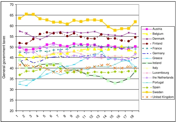
for OECD and EU-15 countries by taking two-year intervals. Focusing on the last 16 years,

we present the tax burden for the 23 0ECD countries in Figure 2.

This paper follows the stream of economists which insists on downsizing government,

although this is an intricate issue as the civil servants themselves have many political powers

(Buchanan and Tullock, 1977). In Section 1, we explain the arguments for downsizing the

goverment by the so-called ‘Armey curve’ (Armey 1995). The conceptual starting point is a

society without a government. The absence of government allows lawlessness, insecurity and

instability. Even a small government could advance welfare by introducing the protection

of property rights and the rule of law. But the richer society gets, the more government

gets involved (Slemrod et al. 1995). The median voter prefers state-of-the-art health care,

education and pension systems. As the scope of the government grows, so do the tax burden

and public expenditures. Public choice theory predicts that governments will expand in

size beyond its e¢cient level: higher public expenditures result in a lower GDP growth.

Advocates of the Armey curve try to estimate the e¢cient level of government involvement.

They obtain optimal values which are lower than the current observations.

drawbacks which are circumvented by the non-parametric estimation in Section 2. Using Data

Envelopment Analysis (DEA), we develop an alternative approach to determining the optimal

size of the government. By applying an input-oriented model (i.e., minimization of the inputs

for a given output level) on a sample of 23 OECD countries, we benchmark governments by

comparing GDP growth relative to their tax burdens. In a …rst stage analysis, we investigate

the variables as proposed by Armey (1995). We measure the size of the government by

overall government spending (general government outlays). These expenditures include the

spendings from the central, state and local government as well as spendings by the social

security system (cfr. Guptaet al. 2001). Other measures of government size are also popular. Meltzer and Richard (1981) use the share of income redistributed by government as a measure

of relative size. Katsimi (1998) de…nes the size of the public sector as the ratio of public to

total employment. Others use the total tax level or the share of government consumption

in total consumption. As these measures of government size are strongly correlated (e.g.,

correlation of 0.88 between public spending and overall taxation level), our results remain

robust for related measures.

In a second stage, we correct the …rst stage gross e¢ciency measures. As a …rst correction

variable, we develop the idea of the anorexia family. Countries with lean family sizes prefer larger government involvement, since the public sector takes over several concerns which used

to be handled within the family. Family size is considered as an implicit revelation of the

preference for the extent of government involvement. Other correction factors are openness

of the economy (Roderik 1996), initial GDP per capita to capture the catching up e¤ect

(Wagner 1877) and the income of the median voter, urbanization, country size (proxied by

the total population), population density and the capital stock (proxy of physical capital

stock).

In methodological terms, this paper develops a simple procedure to correct the DEA

e¢-ciency scores for environmental characteristics by using the residuals of the Tobit regressions.

We extend the procedure as suggested by Gasparani and Ramos (2003) to a more generous

correction mechanism. The optimal size of the public sector is computed as the actual size

Tax burden 20 25 30 35 40 45 62-63 66-67 70-71 74-75 78-79 82-83 86-87 90-91 94-95 98-99 02-03 years ta x a s % o f GD P

OECD 2 year EU-15 2 year

Figure 1: Tax burden 1962-2003

times the adjusted net e¢ciency score. We do not consider the in‡uences of outliers nor

measurement errors. From the outset, it should be emphasized that our approach o¤ers only

a partial analysis. As such, we do not investigate the crucial issue of equity, i.e., the

in-terpersonal redistribution of opportunities, income and wealth. Furthermore, in the context

of political economy, the many dimensions of ‘eudemonia’ (good life and happiness) are not

covered except for the contribution from real growth.

Our results show that, on average, the public sector of the 23 OECD countries which

constitute our sample should decrease by 3.74 percentage points to reach an overall tax

burden of 41.22% of GDP. The Italian public sector, followed by the Swedish, would be

prone to the largest decrease with, respectively, 10.24 and 7.88 percentage points. Public

spending in New Zealand appears to be too low and could thus increase.

1

Is there an optimal government size?

1.1

The Armey curve

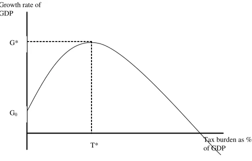
The search for an optimal size of government has been popularized by Armey (1995). The

so-called ‘Armey curve’, which is represented in Figure 3, describes the relationship between

20 25 30 35 40 45 50 55 60 65 70

1 2 3 4 5 6 7 8 9 _{10 11 12 13 14 15 16 17 18}

G ener al gover nm ent t axes Austria Belgium Denmark Finland France Germany Greece Ireland Italy Luxembourg the Netherlands Portugal Spain Sweden United Kingdom

Figure 2: Tax burden for some OECD countries

If the government has no resources (i.e., zero taxation level), the growth rate of the economy

corresponds to G0. In a world without rule of law, private agents have to protect their

own property rights. The establishment of a government skims some income, but creates a

higher growth rate by introducing the provision of public goods and services which increases

overall economic e¢ciency. At low levels of government spending, an increase in the tax rate

raises the growth rate since the outlays (e.g., for infrastructure, education, public health,

protection of property) are considered to be productive (Scully 2003). However, whereas

the …rst euros spent have huge marginal e¤ects, the next euros have smaller e¤ects. For

example, once a country possesses primary roads, the positive e¤ects of secondary roads are

smaller. In addition, as higher taxes are needed to …nance government, distortions usually

become more prevalent. Agents change their behavior in order to escape taxes. Public choice

theory also predicts that the government o¢cials become increasingly self-interested and not

benevolent (see Mueller (2003) for an overview). Therefore, the curve has a concave shape

due to decreasing marginal returns: a proportional increase in spending and taxation yields

a less than proportional increase in economic growth. But thanks to positive externalities,

an additional percentage of tax burden still creates higher economic e¢ciency (i.e., a positive

T* G*

Tax burden as % of GDP Growth rate of

GDP

G0

Figure 3: Armey curve

slope).

At some point, the marginal bene…ts from increased government spending become zero.

With a tax burden of T , the government induces the highest possible rate of economic

growth. BeyondT , government spending is more oriented towards non-productive spending

(e.g., transfers and subsidies). An increase in the tax rate then lowers the growth rate of the

economy. In contrast with what has come before, the additional resources claimed by the

government come at the cost of private projects with higher returns.

1.2

Estimation of the optimal government size

The empirical literature provides several attempts to estimate the optimal level of the public

sector. We mention some studies. Based on a model of endogenous growth, Barro (1990) …nds

the growth maximizing tax rate to be 25.1%. However, the standard error of the coe¢cient

is so large that con…dence in the estimate is quite small. Chao and Grubel (1998) place

the maximum of the Armey curve for Canada at 34% of GDP. Pevcin (2004) suggests that

the Armey curve for 12 European countries peaks when government spending is between

36.6% and 42.1% of GDP. Scully (1994) estimated a curve similar to the Armey curve. His

model yields an optimal tax burden of 19.3% of GDP for the United States and 23% for

is 22.5%, far below the observed tax burden of 28%. Afonso et al. (2006) calculate that

countries with lean public sectors and with public expenditure ratios of about 30% of GDP

tend to be the most e¢cient countries in terms of public performance. As we show below,

our results are somewhat similar, in that we estimate the average optimal size for the OECD

countries to be around 40% of GDP with a standard deviation of 5%.

1.3

Drawbacks of a parametric estimation

Although the Armey curve represents an attractive conceptual framework, it su¤ers from a

few drawbacks which make an empirical estimation of the curve rather inadequate. Some

authors (e.g., Pevcin 2004) estimate the Armey curve by using a panel dataset in which the

space and time dimension are disregarded. Measuring the optimum in this way assumes

that all countries have the same G0, as well as the same preferences and the same rate of

decreasing marginal returns (Slemrod et al. 1995). These assumptions seem unrealistic.

Moreover, the social cost of raising revenues, as well as their social bene…ts, can be expected

to vary among countries due to di¤erences in the e¤ectiveness of budgetary institutions

and political economy factors. In some countries, for example, citizens favor redistributive

policies, while in others, they do not (Guptaet al. 2001).

If the Armey curve is estimated by country speci…c time series as in, e.g., Scully (2001),

correlation is confused with causation. During periods of more robust economic growth, as

in the 1950s and 1960s, government involvement was rather modest. Governments enlarged

their outlays in the 1970s and 1990s when economic growth slowed down. However, this

negative correlation does not necessarily mean causation. On the one hand, economic growth

is subject to many exogenous factors (see, e.g., Crafts and Toniolo (1996)); on the other hand,

government involvement is the result of the aggregation of social preferences in society, which

varies with the voting rules in place. Estimations such as those by Scully (2001) do not take

these e¤ects into account.

In addition, parametric models assume a priori a particular functional form on the

dataset, which is di¢cult to justify. We suggest an alternative exploration by estimating the

optimal tax burden by use of the non-parametric ‘Data Envelopment Analysis’ (DEA). This

procedure allows us to compare governments and to benchmark their long term achievements.

We are able to correct for control variables, such as the openness of a country or preferences

about government involvement in the economy (see infra). In this paper, we follow a

top-down approach as explained in Slemrod et al. (1995). Top-down studies investigate the overall association between government involvement and economic growth. They contrast

with bottom-up studies which estimate costs country by country, program by program and

tax by tax.

2

Measuring government size with DEA

2.1

Measuring with DEA

Data envelopment analysis (DEA) assesses the relative e¢ciency of decision making units

(DMUs). The original model with constant returns to scale was proposed by Charnes, Cooper

and Rhodes (CCR) (1978) and later extended by Banker, Charnes and Cooper (BCC) (1984)

to variable returns to scale. The DEA approach de…nes a non-parametric frontier which

serves as a benchmark for e¢ciency measures. The frontier is constructed as the piecewise

linear combination of the e¢cient DMUs in the sample.

We consider the input-oriented model which searches for the minimal inputs needed to

produce given outputs. The e¢ciency of a DMU is obtained as the maximum of the ratio of

the weighted sum of its outputs to the weighted sum of its inputs, subject to the condition

that this ratio for any DMU does not exceed 1. This condition means that no DMU can operate beyond the e¢ciency frontier. We further assume non-negative weights. If there

are m inputs xi, s outputs yr and n DMUs (indexed by j " f1;2; : : : ; ng), we state the BCC-problem as a simple linear programming formulation:

k(x; y) = j xo n

P

i=1 i

xi;yo n

P

i=1 i

yi; i 0; n

P

i=1 i

= 1;i= 1; :::; n (1)

The inputs and outputs, labelled with aisubscript, are the inputs and outputs ofDM Ui

technical e¢ciency score ofDM Ui is de…ned as the value of i. If i equals 1, the DMU is

relatively e¢cient. If i is less than 1, it could produce, given its inputs, (1 i) percent

more outputs. We consider i as a gross e¢ciency measure which we will further correct for

control variables in order to obtain an adjusted net e¢ciency measure.

Consider the case where there is only one input variable in an input-oriented model.

Multiplying the e¢ciency score i by the only input value, we obtain the targeted input

value. This targeted input value indicates the optimal input for the DMU, given its output.

We compute the optimal size of the government by the use of this optimal target value.

2.2

Advantages of DEA

To our best knowledge, the optimum of the Armey curve has been estimated only by the use

of parametric methods. In this contribution, we apply an input-oriented DEA model to the

problem (i.e., minimization of the inputs for a given amount of outputs). Although one of the

advantages of DEA is the use of multiple inputs and outputs, we compute the model only for

one input and one output variable. The tax burden is used as the input variable, and GDP

growth as the output variable. This is consistent with the idea behind the Armey curve: for

a given GDP growth rate, what is the optimal level of tax burden? By the use of DEA, we

calculate for every country an optimal government size relative to the observed performances

of the other countries in the dataset. In other words, we benchmark the governments by

relating a country’s economic growth to the size of its government. Since DEA is a

non-parametric estimation procedure, we do not need any a priori assumption about the shape of the production function, as is required in the literature estimating an inverted U-shape.

Moreover, in a second step, we will take into account control variables (e.g., openness of the

country) and preferences (e.g., redistribution towards families).

The analysis covers OECD economies. Studying only OECD countries o¤ers several

advantages (see, e.g., Alesina and Furceri 2008). Firstly, data quality and comparability

are of higher standards. Comparability is the more important due to the relative nature

of the DEA technique. Secondly, data from OECD and non-OECD countries do not share

a common set of coe¢cients in growth regressions (Grier and Tullock 1989). As such, it is

di¢cult to pool these data. Finally, and related to the previous point, the economic structures

in emerging OECD countries di¤er from those in mature economies. Therefore, we considere

a sample of 23 reasonably comparable OECD countries. We borrow the data from the

OECD statistical databases and evaluate the year 1999 (due to data constraints for family

size, see infra). Nevertheless, we experimented with other years as well. As mentioned earlier, the output variable is GDP growth.1 _{Gross Domestic Product (GDP) is preferred}

above Gross National Product (GNP) as GDP yields a better correlation with the economic

activity within a country. The degree of government involvement is measured by the level of

general government spending (total outlays). General government spending is the sum of the

spendings by the central, state and local government, as well as social security spendings.

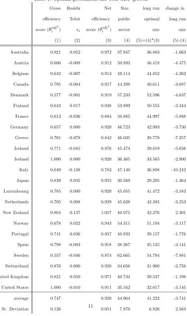
The input-oriented e¢ciency scores are presented in the …rst column of Table 1. We learn

from this exercise that Ireland and the United States allocate the levied taxes most e¢ciently.

For a given GDP growth, their governments need the smallest tax absorption. The Swedish

and Danish governments spend according to the gross e¢ciency scores the collected taxes in

the least e¢cient way in order to push GDP. The average gross e¢ciency score is 0.75. This

means that, if governments would perform e¢ciently (i.e., as the US and Irish governments),

they would only need 75% of the current taxation level.

3

Correction for exogenous in‡uences

To improve the comperability of the sample, we make corrections for preferences and some

other control variables. By the use of a specially designed econometric procedure, we correct

the gross e¢ciency scores to obtain net e¢ciency values. We …rst introduce and explore the

Table 1: Optimal government size with GDP growth

Gross Residu Net Size long run change in

e¢ciency Tobit e¢ciency public optimal long run

score ( adj

0

i ) i score (

adj3

i ) sector size size

(1) (2) (3) (4) (5)=(4)*(3) (5)-(4)

Australia 0.921 0.052 0.972 37.947 36.883 -1.063

Austria 0.606 -0.008 0.912 50.893 46.418 -4.475

Belgium 0.642 -0.007 0.913 49.114 44.852 -4.262

Canada 0.795 -0.004 0.917 44.298 40.611 -3.687

Denmark 0.577 -0.001 0.919 57.233 52.596 -4.637

Finland 0.643 0.017 0.938 53.899 50.555 -3.344

France 0.612 -0.036 0.884 50.885 44.997 -5.888

Germany 0.657 0.000 0.920 46.723 42.993 -3.730

Greece 0.701 -0.078 0.842 46.035 38.778 -7.257

Iceland 0.771 -0.045 0.876 45.474 39.819 -5.656

Ireland 1.000 0.000 0.920 36.465 33.565 -2.900

Italy 0.649 -0.138 0.783 47.140 36.898 -10.242

Japan 0.839 0.035 0.955 30.569 29.205 -1.364

Luxembourg 0.785 0.000 0.920 45.055 41.472 -3.583

Netherlands 0.705 0.008 0.929 45.638 42.385 -3.253

New Zealand 0.804 0.137 1.057 40.075 42.376 2.301

Norway 0.678 0.022 0.943 54.311 51.194 -3.117

Portugal 0.741 0.036 0.957 40.933 39.157 -1.776

Spain 0.798 -0.003 0.918 38.267 35.125 -3.141

Sweden 0.557 -0.046 0.874 62.665 54.784 -7.881

Switzerland 0.876 0.000 0.920 34.656 31.900 -2.756

United Kingdom 0.821 0.050 0.971 40.734 39.537 -1.198

United States 1.000 -0.010 0.911 35.162 32.017 -3.145

average 0.747 0.920 44.964 41.222 -3.741

3.1

The anorexia family

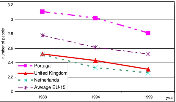
Family size in OECD countries steadily decreased during the last few decades. Whereas

an average family consisted of 2.8 members in 1988, eleven years later a typical family has

only 2.5 members (see Figure 4). One could say that the anorexia family emerges. The

question remains as what extent this decline in family size re‡ects government involvement.

Empirically, we …nd a strong negative correlation (-0.80) between family size and overall

government taxes measured as a percentage of GDP and between family size and government

spending (-0.55) (see Figure 5 for 1999 data).

On the one hand, the anorexia family invites the government to take up more tasks.

Whereas before, for instance, families themselves looked after their younger and older

mem-bers, crèches and resthomes supported by the government often ful…l that requirement

nowa-days. Several tasks which formerly were family responsibilities are nowadays assigned to the

welfare state. On the other hand, thanks to extended government involvement, families could

emaciate. Governments provide, for instance, pension allowances such that children are no

longer the only safeguards for retired parents.2

Although we …nd a strong correlation, we do not know the direction of the causality.

In further research, this causality should be carefully examined by Instrumental Variables

(IV) techniques.3 _{To present a ‡avor of the correlation between the family size and the}

government size, by use of an ordinary least squares estimation, we test the hypothesis that,

for 23 OECD-countries, a smaller family size yields a larger government involvement. The

results are presented in Table 2. Family size alone can explain 30.5% of the variation in

taxation levels. We also checked whether the results remain robust if we add per capita GDP

as an explanatory variable.

There exists a large and growing public …nance literature on the relationship between

government involvement and family size. A large part of the literature focuses on the link

between fertility, growth and government size. This branch is based on the inspiring paper

of Galor and Weil (1996). Another branch of the literature discusses the role of family size

2 2.2 2.4 2.6 2.8 3 3.2

1988 1994 1999 year

number

of

peopl

e

Portugal United Kingdom Netherlands Average EU-15

Figure 4: Family size 1988-1999

knowledge the literature does not provide a model which speci…es the relationship between

family size and the size of the government.

In the remainder of this section, we consider family size to represent an implicit

prefer-ence for the extent of government involvement. Societies which prefer a larger government

involvement (e.g., Denmark with general government spending equal to 52.5% of GDP in

1999), have on average smaller families (i.e., Denmark counts only 2.14 members in 1999).

Due to the unknown causality is the reverse also true: societies with lean public sectors

(e.g., Spain with 38.3% of GDP), have on average bigger families (i.e., Spain counts 3.24

family members). If we consider total ‘social’ expenditures, which are measured as the sum

of resources spend for families, disabled persons, the unemployed, elderly people and sick

persons, as an explicit measure for government involvement, we …nd a signi…cant negative

correlation (-0.65) between explicit and implicit preferences. Family size can explain 38.5%

of the variation in total social expenditures (see Table 3 and Figure 6).

3.2

Other control variables

The countries in the sample di¤er in several aspects. First of all, di¤erent countries have

di¤erent tastes and preferences about the optimal size of government. We capture preferences

UK Sweden Finland Portugal Austria Netherlands Luxembourg Italy Ireland France Spain Greece Germany Denmark Belgium 25 35 45 55 65

2 2,2 2,4 2,6 2,8 3 3,2 3,4

family size (1999)

G ov er nm ent s pending (1999)

Figure 5: The anorexia family and government spending

United States United Kingdom Switzerland Sweden Spain Portugal Norway New Zealand Netherlands Luxembourg Japan Italy Ireland Iceland Greece Germany France Finland Denmark Canada Belgium Austria Australia 10 15 20 25 30 35

2 2,2 2,4 2,6 2,8 3 3,2 3,4

Family size (1999)

T ot al s oc ial ex pendi tures (1999)

Table 2: Relationship government size - family size

Dependent variable: logarithm of average taxes levied by general government

Variable Coe¢cient Std. Error

Constant 4.6027 *** 0.2744

Family size -0.3277 *** 0.1080

R-squared 0.3049

where *** denotes signi…cance at 1% level.

Table 3: Relationship social expenditures - family size

Dependent variable: logarithm of total social expenditures

Variable Coe¢cient Std.Error

Constant 4.3218 0.3424

Familysize -0.4889 0.1347

R-squared 0.3854

where *** denotes signi…cance at 1% level.

for the extent of government involvement by the average family size. Countries with lean

families prefer larger government involvement as argued in the previous section.

Secondly, we correct for the degree of countries’ openness to trade. Open countries are

more subject to external shocks and therefore need a larger public sector to accomplish a

stabilizing role (Roderik 1996). We measure the degree of openness by computing the sum of

exports and imports as a percentage of GDP. Afonsoet al. (2006) remark that exports also

can act as a proxy for the degree of international competition in labor and capital markets,

and that greater competitiveness would penalize public ine¢ciency disproportionately. If

the penalizing e¤ect of Afonso et al. (2006) dominates, we expect a positive sign in the correction, if Roderik’s stabilizing requirement dominates, we expect a negative sign.

A third correction measure is GDP per capita. It captures the large income elasticity

(exceeding one) with respect to governmental services as suggested by Wagner (1877). He

stated that richer economies prefer larger public sectors. In addition, GDP per capita is also

a measure for the income of the median voter4 (although median income is more usual), who

is an important actor in the public choice literature (starting from Tullock 1972; Borcherding

and Deacon, 1972).

Fourthly, we include the capital stock of a country. This variable aims to proxy the physical

capital stock which stimulates an e¢cient production of (public) goods and services (Afonso

et al. 2006).

Finally, we include some traditional variables to explain government involvement: country

size (expressed as total population), population density and urbanization (proxied by the

share of national population in the 10% of regions with the largest populations).

In order to compute the adjusted net e¢ciency score for each DMU, we econometrically

explore these factors which are likely to in‡uence productive e¢ciency. The left-hand variable

is the gross e¢ciency score, while the right-hand variables are the correction factors. Since

the gross e¢ciency scores are right-censored (no values above 1), we have to estimate by

a Tobit model. The regression residuals from the Tobit model indicate the portion of the

e¢ciency that remains unexplained after correcting for the control variables (Tupper and

Resende 2004). Since the residuals alternate in sign, whereas a proper e¢ciency measure

should possess a one-sided distribution, we use the procedure of Gasparini and Ramos (2003),

which allows us to generate adjusted DEA scores that are con…ned within the[0;1]interval:

adj

i = i+ (1 max

j=1;:::;n j) (2)

where adji denotes the adjusted e¢ciency score forDM Ui, istands for the residual for each

DM Ui obtained from the Tobit estimation.

However, we consider this procedure as ‘too severe’. Some governments could be

‘inef-…cient’ simply because they are too small. Those governments could, by increasing the tax

burden, obtain a larger GDP growth. The adjusted e¢ciency score as obtained by

equa-tion (2) fails to detect those ine¢cient governments. Therefore, we extend the procedure of

Gasparini and Ramos (2003) to a more general correction mechanism. Our suggestion is to

consider not only the largest residual, but an average of the wlargest residuals. Hence, we

sort the residuals i in order of magnitude and compute:

adjw

i = i+ (1

1

w w

X

j=1

j): (3)

residuals are corrected. The larger is w, the less severe is the correction and, hence, the

larger is the average optimal public sector. As we do not know the proper value of w, we

further perform a sensitivity analysis.

3.3

Sizing the government

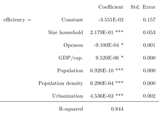
The results of the estimation are given in Table 1. The left column in the Table represents

the uncorrected gross e¢ciency scores. By estimating a Tobit regression, we correct the gross

e¢ciency scores. The Tobit estimation is presented in Table 4. Family size, openness of the

economy, country size, population density and urbanization have a statistically signi…cant

e¤ect on the e¢ciency of the DEA model. As capital stock has a very insigni…cant e¤ect, we

removed it from the results. Family size has the expected positive e¤ect on gross e¢ciency.

The larger the average family, the higher the gross e¢ciency. Hence, countries with larger

average family size (and thus preferences for less government involvement), can create a

given GDP growth with fewer government spendings. Since larger exports decrease e¢ciency,

Roderik’s stabilizing e¤ect emerges. GDP per capita shows a positive but insigni…cant e¤ect

on the e¢ciency: the richer the country, the higher the gross e¢ciency. Both country size,

population density and urbanization in‡uence the gross e¢ciency scores positively.

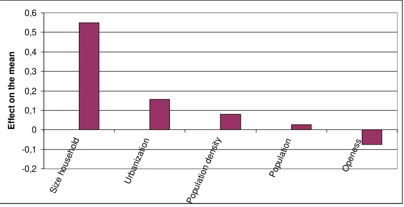
As also the size of the e¤ect is of importance, we present in Figure 7 the e¤ect on the

mean of each of the signi…cant variables. We observe that the e¤ect of the household size

has the largest in‡uence on e¢ciency. Urbanization, population density and population have

clearly a lower e¤ect on the mean.

Since we are primarily interested in the residuals which we obtain from the Tobit

regres-sion, the …nding whether a certain variable has a signi…cant impact on the e¢ciency score

does not matter so much for our purpose. The residuals are reproduced in the second column

of Table 1. From the residuals, we compute the net e¢ciency scores by use of equation (3)

with w arbitrarily set to, e.g., 3 (later on, we perform a sensitivity analysis). The optimal

size is computed as the government size times the adjusted net e¢ciency score.

From comparing the gross and the net e¢ciency scores, we learn that all countries, except

for Ireland and the United States, gain from the correction for control variables. The e¢ciency

scores of Denmark, Sweden and Austria increase the most, thanks to the correction for

redistributive preferences. If we take control factors into account, the optimal average tax

burden of the 23 OECD countries should amount to 41.22% of GDP. The public sector

thus should on average decrease by 3.74 percentage points. Note that our results compare

well with those in related literature (e.g., Chao and Grubel 1998 or Pevcin 2004). But the

optimal government size di¤ers considerably between the countries. The largest decrease in

tax burden should occur in Italy, with a fall of 10.24 percentage points. Also Sweden, Greece,

Iceland and France should decrease the tax burden by more than 5 percentage points. In

contrast, the tax burden in New Zealand should optimally increase by 2.30 percentage points

to 42.37% of GDP.

Table 4: Tobit estimation with GDP growth

Coe¢cient Std. Error

e¢ciency = Constant -3.551E-02 0.157

Size household 2.179E-01 *** 0.053

Openess -9.100E-04 * 0.001

GDP/cap. 9.520E-06 * 0.000

Population 6.920E-10 *** 0.000

Population density 6.290E-04 *** 0.000

Urbanization 4.536E-03 *** 0.002

R-squared 0.844

where *** denotes e¢ciency at 1% level, ** at 5% and * at 10%.

In order to test the robustness ofw in determining the size of the optimal government

involvement, we perform a sensitivity analysis. We compute for several values of w the

optimal tax burden. The results are presented in Table 5. Notice that, as w increases, the

optimal size of government rises as well. The di¤erence between adj 1

i and adj7

i amounts

on average to 3.92 percentage points. However, some countries bene…t more from generous

-0,2 -0,1 0 0,1 0,2 0,3 0,4 0,5 0,6

Size househol

d

Urbani zat

ion

Pop ulat

ion densi

ty

Pop ulat

ion

Openess

Eff

ect

on

the

m

ean

Figure 7: E¤ect on the mean of the exploratory variables

points. Sweden is followed by Denmark (a di¤erence of 4.98), Norway (4.72) and Finland

(4.69). These Scandinavian countries take most advantage of a more generous weighting of

w. Japan (with 2.66) obtains the least gain from the weighting system.

However, even in a very generous model (i.e., w equal to 7), most governments would

have to decrease spending by 2.41 percentage points in order to obtain higher GDP growth.

Only New Zealand should decrease its tax burden in none of the models. Australia and

United Kingdom should optimally increase the government size from the moment we correct

by takingwas 7.

3.4

Public sector performance

Economic growth is not the only objective that a benevolent government can pursue.

Mus-grave (1959) de…ned three major tasks for the government: (1) allocative e¢ciency, (2)

economic stability and (3) redistribution. Afonso et al. (2005) added to these main tasks four opportunity indicators: the quality of administration, education, health and public

in-frastructure. The last four indicators describe the rule of law and the promotion of equality

and opportunity in the market place. Afonso et al. (2005) constructed the composite

Table 5: Sensitivity analysis

Actual size adj

1

i

adj2 i

adj3 i

adj4 i

adj5 i

adj6 i

adj7 i

Australia 37.947 34.704 36.326 36.883 37.295 37.551 37.803 38.008

Austria 50.893 43.496 45.670 46.418 46.970 47.314 47.652 47.927

Belgium 49.114 42.031 44.130 44.852 45.384 45.716 46.042 46.307

Canada 44.298 38.067 39.960 40.611 41.092 41.391 41.685 41.924

Denmark 57.233 49.310 51.755 52.596 53.217 53.604 53.983 54.293

Finland 53.899 47.460 49.763 50.555 51.140 51.504 51.861 52.152

France 50.885 42.075 44.249 44.997 45.549 45.893 46.230 46.505

Germany 46.723 40.309 42.306 42.993 43.499 43.815 44.125 44.377

Greece 46.035 36.135 38.102 38.778 39.278 39.589 39.894 40.143

Iceland 45.474 37.207 39.150 39.819 40.312 40.619 40.921 41.166

Ireland 36.465 31.471 33.029 33.565 33.961 34.207 34.449 34.646

Italy 47.140 34.191 36.205 36.898 37.409 37.728 38.040 38.295

Japan 30.569 27.449 28.755 29.205 29.536 29.743 29.946 30.111

Luxembourg 45.055 38.884 40.809 41.472 41.960 42.265 42.564 42.807

Netherlands 45.638 39.764 41.714 42.385 42.880 43.189 43.491 43.738

New Zealand 40.075 40.075 41.787 42.376 42.811 43.081 43.347 43.564

Norway 54.311 48.075 50.395 51.194 51.783 52.150 52.510 52.803

Portugal 40.933 36.807 38.556 39.157 39.601 39.878 40.149 40.370

Spain 38.267 32.928 34.563 35.125 35.540 35.799 36.053 36.259

Sweden 62.665 51.185 53.863 54.784 55.464 55.887 56.303 56.641

Switzerland 34.656 29.909 31.390 31.900 32.275 32.510 32.739 32.927

United Kingdom 40.734 37.197 38.938 39.537 39.979 40.254 40.524 40.744

United States 35.162 29.997 31.500 32.017 32.398 32.636 32.869 33.059

average 44.964 38.640 40.561 41.222 41.710 42.014 42.312 42.555

maximum 62.665 51.185 53.863 54.784 55.464 55.887 56.303 56.641

minimum 30.569 27.449 28.755 29.205 29.536 29.743 29.946 30.111

cator ‘Public Sector Performance’ (PSP) by equal weighting of these seven sub-indicators.

We investigate whether the optimal size of the government changes if we use the

PSP-indicator in the …rst step of the DEA-model. In this setting, the government has to minimise

spending, while ful…lling a whole set of public activities. In the DEA input-model,

govern-ment spending remains the input, while PSP becomes the output variable. Once more we

correct for implicit preferences (family size as proxy), openness, GDP per capita, country

size, population density and urbanization. The results are given in Table 6.

Table 6 with PSP as output in the …rst step, slightly di¤ers from Table 1 with GDP growth

as output in the initial DEA-model. The correlation is 0.93. Whereas the average size of

the government was 41.22%, an extension to broader government tasks yields an optimal

tax burden of 42.18%. Again we compute the di¤erence between the actual size and the

long run optimum. The Italian public sector should reduce its resources the most. It should

optimally decrease its spending by 9.22 percentage points. Sweden, Germany, France and

Finland complete the top-…ve biggest declines. Norway, New Zealand, Australia and United

Kingdom should optimally enlarge their public sector to meet the PSP criteria even better.

The di¤erence between the two models is largest for Norway. The optimal Norwegian

spendings are 8.27 percentage points higher, if measured by PSP. The German government

involvement should optimally be 3.18 percentage points smaller if measured by GDP growth

as output variable in the …rst step. There is almost no di¤erence between the two procedures

for the United States (0.15 percentage points larger if measured by PSP as output in the …rst

step) and Switzerland (0.11).

4

Concluding remarks

Government involvement expanded rapidly in the second part of the last century. Many

economists insist on downsizing the government. Their arguments are based on the

so-called ‘Armey curve’. We indicate that these estimates rely on unrealistic assumptions, the

ignorance of preferences and a confusion of correlation with causation. We …nd a strong

negative correlation between family size and overall government size. On the one hand,

Table 6: Optimal government size with PSP

Gross Residu Net Size long run change in

e¢ciency Tobit e¢ciency public optimal long run

score ( adj

0

i ) i score (

adj3

i ) sector size size

1 2 3 4 5 = 4*3 5 = 4

Australia 0.959 0.104 1.060 35.714 37.851 2.137

Austria 0.606 -0.042 0.914 50.222 45.894 -4.328

Belgium 0.642 0.038 0.994 47.593 47.303 -0.290

Canada 0.785 -0.032 0.924 42.935 39.688 -3.247

Denmark 0.577 0.015 0.971 56.160 54.514 -1.646

Finland 0.643 -0.037 0.919 54.501 50.092 -4.409

France 0.612 -0.051 0.905 49.136 44.486 -4.650

Germany 0.657 -0.067 0.889 44.779 39.808 -4.971

Greece 0.701 -0.061 0.895 40.716 36.440 -4.276

Iceland 0.771 0.012 0.968 42.084 40.728 -1.356

Ireland 0.963 0.005 0.961 38.414 36.898 -1.515

Italy 0.649 -0.160 0.796 45.290 36.070 -9.220

Japan 1.000 0.040 0.996 31.673 31.537 -0.136

Luxembourg 0.891 0.000 0.956 46.379 44.338 -2.041

Netherlands 0.705 0.023 0.979 46.675 45.693 -0.983

New Zealand 0.795 0.112 1.068 44.113 47.093 2.979

Norway 0.678 0.116 1.072 55.491 59.466 3.975

Portugal 0.741 0.008 0.964 38.871 37.463 -1.407

Spain 0.791 -0.018 0.938 38.671 36.291 -2.380

Sweden 0.551 -0.084 0.872 61.829 53.891 -7.938

Switzerland 0.876 0.000 0.956 33.253 31.789 -1.463

United Kingdom 0.821 0.054 1.010 40.166 40.580 0.413

United States 1.000 0.003 0.959 33.537 32.173 -1.364

Table 7: Tobit estimation with PSP

Coe¢cient Std. Error

e¢ciency = Constant 2.553E-01 0.163

Size household 9.142E-02 0.064

Openess -9.640E-04 0.001

GDP/cap. 5.270E-06 *** 0.000

Population 1.110E-09 ** 0.000

Population density 4.820E-04 ** 0.000

Urbanization 5.956E-03 *** 0.002

R-squared 0.763

where *** and ** denote, respectively, signi…cance at 1 and 5% level.

the anorexia family forces the government to take up more tasks. On the other hand, as

government involvement expands, families could emancipate.

We estimate by the use of a non-parametric ‘Data Envelopment Analysis’ (DEA) the

gross e¢ciency of government spendings (1999 data). In a second stage, these gross-scores

are corrected by linking them to classic control variables such as initial per capita income

(Wagner 1877), degree of openness (Roderik 1996), country size, population density and

urbanization. We introduce family size as a novel explanatory variable. By the use of a

generous correction mechanism, we compute the optimal size of the government. The optimal

average government involvement in the 23 OECD countries amounts to 41.22% of GDP. This

means that the public sector should on average decrease by 3.74 percentage points. Whereas

the largest decrease should occur in Italy with a reduction of 10.24 percentage points, New

Zealand should optimally increase its government involvement by 2.30 percentage points.

Borrowing the composite indicator ‘Public Sector Performance’ (PSP) of Afonsoet al. (2005), we enlarge the objectives of a benevolent government beyond economic growth. It

appears that the average optimal tax burden slightly increases to 42.17%. However, Italy

and Sweden should still decrease their government involvement by more than 5 percentage

points.

Acknowledgements

We are grateful to Bart Capéau, Laurens Cherchye, Koen Decancq, Blanca Zuluaga, James

Gibb, two anonymous referees, the Editor in Chief of Public Choice and participants at the

OR48 Conference in Bath University for their helpful comments.

Notes

1_{In order to …lter out the economic cycles from the raw data, we take the arithmetic mean of real GDP}

growth for the period 1988 - 2004. The variable thus obtained reads as the long-run GDP growth.

2_{Remark that when government taxes are considered as a proxy for the government size, the causation}

could be in‡uenced by the design of the tax system. For a speci…c tax system, a larger family size could

reduce government revenues.

3_{In the current research, we do not examine the causality formally as (1) the appropriate techniques are}

not available in the non-parametric DEA and as (2) selecting the appropriate IV are an intricate issue.

4_{Indeed, thanks to the law of large numbers we approximate a normal distribution, such that, the median}

value converges to the mean value.

References

[1] Afonso, A., Furceri, D. (2008). Government size, composition, volatility and economic

growth.ECB Working Paper Series 849, p. 45.

[2] Afonso, A., Schuknecht, L., Tanzi, V. (2005). Public sector e¢ciency: an international

comparison.Public Choice 123, 321-347.

[3] Afonso, A., Schuknecht, L., Tanzi, V. (2006). Public sector e¢ciency, Evidence for new

EU member states and emerging markets.ECB Working Paper Series 581, p. 47.

[4] Alesina, A. ,Wacziarg, R. (1998). Openness, country size and government.Journal of

Public Economics 69, 305-321.

[6] Banker, R., Charnes, A.,Cooper, W. (1984). Some models for estimating technological

and scale ine¢encies in data envelopment analysis.Management Science 30, 1078-1092.

[7] Barro, R. (1990). Government spending in a simple model of endogenous growth.Journal

of Political Economy 95 (5), 103-125.

[8] Barro, R. (1991). Economic growth in a cross-section of countries.Quarterly Journal of

Economics 106 (2), 407-443.

[9] Baumol, W. (1967). Macroeconomics of unbalanced economic growth: the anatomy of

the urban crisis.American Economic Review 57, 415-426.

[10] Borcherding, T.E., Deacon, R.T. (1972). The demand for the services of non-federal

governments.American Economic Review 62 (5), 891-901.

[11] Branson, J., Lovell, K. (2001). A growth maximising tax structure for New Zealand.

International Tax and Public Finance 8, 129-146.

[12] Buchanan, J., Tullock, G. (1977). The expanding public sector: Wagner squared.Public

Choice31 (1), 147-150.

[13] Chao, J., Grubel, H. (1998). Optimal Levels of Spending and Taxation in Canada, In

Herbert Grubel (ed.). How to Use the Fiscal Surplus: What is the Optimal Size of

Government? Vancouver: Fraser Institute, 53-68.

[14] Charnes, A., Cooper, W., Rhodes, D. (1978). Measuring the e¢ciency of Decision

Mak-ing Units.European Journal of Operational Research 2, 429-444.

[15] Crafts, N., Toniolo, G. (1996).Economic growth in Europe since 1945. Cambridge Uni-versity Press.

[16] Cremer, H., Dellis, A., Pestieau, P. (2003). Family size and optimal income taxation.

Journal of Population Economics 16, 37-54.

[17] Galor, O., Weil, D.N. (1996). The Gender Gap, Fertility, and Growth. American

Eco-nomic Review 86, 374-387.

[18] Gasparini, C., Ramos, F. (2003). Efetividade e e…ciencia no ensino medio brasileiro.

Economia Aplicada 7, 389-411.

[19] Grier, K., Tullock, G. (1989). An empirical analysis of cross-national economic growth:

1951-1980.Journal of Monetary Economics 24, 259-276.

[20] Gupta, S., Leruth, L., Mello, L., Chakravarti, S. (2001). Transition economies: How

appropriate is the size and scope of Government?.IMF Working Papers 55, p. 31.

[21] Higgs, R. (1987). Crisis and Leviathan: Critical episodes in the growth of American

government.Oxford University Press.

[22] Katsimi, M. (1998). Explaining the size of the public sector.Public Choice 96, 117-144.

[23] Lybeck, J., Henrekson, M. (1988).Explaining the growth of government. Amsterdam : North-Holland, p. 396.

[24] Meltzer, A., Richard, S. (1981). A rational theory of the size of government. Journal of

Political Economy 89, 914-925.

[25] Meltzer, A., Richard, S. (1983). Tests of a rational theory of the size of goverment.Public

Choice 41, 403-418.

[26] Mueller, D.C. (2003). Public Choice III. Cambridge University Press, third edition.

[27] Musgrave, R. (1959).The theory of public …nance. McGraw-Hill, New York, p. 161-385.

[28] Niskanen, W. (1971). Bureaucracy and Representative Government. Chicago: Aldine and Atherton.

[29] Pevcin, P. (2004). Does optimal size of government spending exist?. Paper presented

to the EGPA (European Group of Public Administration), 2004 Annual Conference,

Ljubljana, p. 12.

[30] Roderik, D. (1996). Why Do More Open Economies Have Bigger Governments?.NBER

[31] Scully, G. (1994). What is the optimal size of Government in the United States?.NCPA

Policy Report 188, p. 10.

[32] Scully, W. (2001). Government expenditure and quality of life.Public Choice 108, 123-145.

[33] Scully, W. (2003). Optimal taxation, economic growth and income inequality. Public

Choice115, 299-312.

[34] Slemrod, J., Gale, W., Easterly, W. (1995). What do cross-Country studies teach about

government involvement, prosperity and Economic growth?.Brookings papers on

Eco-nomic Activity 2, 373-431.

[35] Tullock, G. (1972). Book review: W. A. Niskanen, Bureaucracy and representative

gov-ernment.Public Choice 12, 119-124.

[36] Tupper, H., Resende, M. (2004). E¢ciency and regulatory issues in the Brazilian water

and sewage sector: an empirical study.Utilities Policy 12, 29-40.

[37] Wagner, A. (1877).Finanzwissenschaft. Leipzig: C.F. Winter.