Munich Personal RePEc Archive
Bootstrapping realized multivariate
volatility measures
Dovonon, Prosper and Goncalves, Silvia and Meddahi, Nour
Concordia University, CIREQ
July 2010
Online at
https://mpra.ub.uni-muenchen.de/40123/
Bootstrapping realized multivariate volatility measures
∗Prosper Dovonon†, S´ılvia Gon¸calves‡ and Nour Meddahi§
Concordia University, Universit´e de Montr´eal and Toulouse School of Economics
July 30, 2010
Abstract
We study bootstrap methods for statistics that are a function of multivariate high frequency returns such as realized regression coefficients and realized covariances and correlations. For these measures of covariation, the Monte Carlo simulation results of Barndorff-Nielsen and Shephard (2004) show that finite sample distortions associated with their feasible asymptotic theory approach may arise if sampling is not too frequent. This motivates our use of the bootstrap as an alternative tool of inference for covariation measures.
We consider an i.i.d. bootstrap applied to the vector of returns. We show that the finite sample performance of the bootstrap is superior to the existing first-order asymptotic theory. Nevertheless, and contrary to the existing results in the bootstrap literature for regression models subject to heteroskedasticity in the error term, the Edgeworth expansion for the i.i.d. bootstrap that we develop here shows that this method is not second order accurate. We argue that this is due to the fact that the conditional mean parameters of realized regression models are heterogeneous under stochastic volatility.
Keywords: Realized regression, realized beta, realized correlation, bootstrap, Edgeworth expan-sions.
1
Introduction
Realized statistics based on high frequency returns have become very popular in financial economics.
Realized volatility is perhaps the most well known example, providing a consistent estimator of the
integrated volatility under certain conditions, including the absence of microstructure noise (see Jacod
(1994), Jacod and Protter (1998), Barndorff-Nielsen and Shephard (2002) and Andersen, Bollerslev,
Diebold and Labys (2003)). Its multivariate analogue is the realized covariance matrix, defined as
the sum of the outer product of the vector of high frequency returns. Two economically interesting
∗We would like to thank Torben Andersen, Tim Bollerslev, Valentina Corradi, Peter Hansen, Andrew Patton and Neil
Shephard for useful comments. This work was supported by grants FQRSC, SSHRC and MITACS. The third author benefited from the financial support of the chair ”March´e des risques et cr´eation de valeur” Fondation du risque/SCOR. Parts of this paper were written while Gon¸calves was visiting the Banco de Portugal, Lisboa, and the Finance department at Stern Business School.
†Economics Department, Concordia University, 1455 de Maisonneuve Blvd. West, H 1155, Montreal, Quebec, Canada
H3G 1M8. Tel: (514) 848-2424 ext. 3479. Email: [email protected].
‡D´epartement de sciences ´economiques, CIREQ and CIRANO, Universit´e de Montr´eal. Address: C.P.6128, succ.
Centre-Ville, Montr´eal, QC, H3C 3J7, Canada. Tel: (514) 343 6556. Email: [email protected]
§Toulouse School of Economics. Address: 21 All´ee de Brienne, 31000 Toulouse, France. Phone: +33 (0)5 61 12 85
functions of the realized covariance matrix are the realized correlation and the realized regression
coefficients. In particular, realized regression coefficients are obtained by regressing high frequency
returns for one asset on high frequency returns for another asset. When one of the assets is the market
portfolio, the result is a realized beta coefficient. A beta coefficient measures the asset’s systematic
risk as assessed by its correlation with the market portfolio. Recent examples of papers that have
obtained empirical estimates of realized betas include Andersen, Bollerslev, Diebold and Wu (2005,
2006), Campbell, Sunderam and Viceira (2009), and Viceira (2007).
Recently, Barndorff-Nielsen and Shephard (2004) (henceforth BN-S(2004)) have proposed an
asymp-totic distribution theory for realized covariation measures based on multivariate high frequency returns. Their simulation results show that asymptotic theory-based confidence intervals for regression and
cor-relation coefficients between two assets returns can be severely distorted if the sampling horizon is not
small enough. To improve the finite sample performance of their feasible asymptotic theory approach,
BN-S (2004) propose the Fisher-z transformation for realized correlation. This analytical
transforma-tion does not apply to realized regression coefficients, which in particular can be negative and larger
than one in absolute value.
In this paper we propose bootstrap methods for statistics based on multivariate high frequency
returns, including the realized covariance, the realized regression and the realized correlation
coeffi-cients. Our aim is to improve upon the first order asymptotic theory of BN-S (2004). We consider
an i.i.d. bootstrap applied to the vector of realized returns. Gon¸calves and Meddahi (2009) have
re-cently applied this method to realized volatility in the univariate context. They also proposed a wild bootstrap for realized volatility with the motivation that intraday returns are (conditionally on the
volatility path) independent but heteroskedastic when log prices are driven by a stochastic volatility
model. In this paper we focus only on the i.i.d. bootstrap for three reasons. First, the results in
Gon¸calves and Meddahi (2009) show that the i.i.d. bootstrap dominates the wild bootstrap in Monte
Carlo simulations even when volatility is time varying. Second, the i.i.d. bootstrap is easier to apply
than the wild bootstrap: the wild bootstrap requires choosing an external random variable used to
construct the bootstrap data whereas the i.i.d. bootstrap does not involve the choice of any tuning
pa-rameter. Third, the i.i.d. bootstrap is a natural candidate in the context of realized regressions driven
by heteroskedastic errors. Indeed, the i.i.d. bootstrap applied to the vector of returns corresponds to a pairs bootstrap, as proposed by Freedman (1981). His results show that the pairs bootstrap is robust
to heteroskedasticity in the error term of cross section regression models. Mammen (1993) shows
that the pairs bootstrap is not only first order asymptotically valid under heteroskedasticity in the
error term, but it is also second-order correct (i.e. the error incurred by the bootstrap approximation
converges more rapidly to zero than the error incurred by the standard normal approximation).
We can summarize our main contributions as follows. We show the first order asymptotic validity
of the i.i.d. bootstrap for estimating the distribution function of the realized covariance matrix and
corre-lation coefficients. Our simucorre-lation results show that the bootstrap outperforms the feasible first order
asymptotic theory of BN-S (2004). For the realized regression estimator, we develop an Edgeworth
expansion of the i.i.d. (or pairs) bootstrap distribution that allows us to study the ability of this
method to provide an asymptotic refinement over the distribution theory of BN-S (2004). We focus on
the realized regression test statistic because existing results in the statistics literature (see Mammen
(1993)) suggest that the pairs bootstrap may be second order correct in this case even under stochastic
volatility. This is not the case for the two other statistics (covariance and correlation coefficients),
where the i.i.d. bootstrap cannot be expected to provide second order refinements due to the fact
that it does not replicate the conditional heteroskedasticity in the data. Thus, we do not analyze their higher order properties in this paper. A wild bootstrap could be used in this case, as in Gon¸calves
and Meddahi (2009).
Contrary to our expectations based on the existing theory for the pairs bootstrap in the statistics
literature, we show that the pairs bootstrap does not provide an asymptotic refinement over the
stan-dard first order asymptotic theory in the context of realized regressions. We contrast our application of
the pairs bootstrap to realized regressions with the application of the pairs bootstrap in standard cross
section regressions. We show that there is a main difference between these two applications, namely
the fact that the parameters describing the conditional mean high frequency returns model (i.e. the
conditional mean of the high frequency returns of one asset conditional on the high frequency returns
of another asset) are heterogeneous. This implies that the score of the underlying realized regression
model is heterogeneous and does not have mean zero (although the mean of the sum of the scores is zero). This heterogeneity implies that the standard Eicker-White heteroskedasticity robust variance
estimator is not consistent in the realized regression context, which justifies the need for the more
involved variance estimator proposed by BN-S (2004). The pairs bootstrap variance coincides with
the Eicker-White robust variance estimator and therefore it does not provide a consistent estimator of
the variance of the scaled average of the scores. This is in contrast with the results of Freedman (1981)
and Mammen (1993), where the score has mean zero by assumption. Nevertheless, the pairs bootstrap
is first order asymptotically valid when applied to a bootstrap t-statistic which is studentized with a
variance estimator that is consistent for the population bootstrap variance of the scaled average of the
scores. Because the bootstrap scores have mean zero, the Eicker-White robust variance estimator can be used for this effect. This implies that the bootstrap statistic is not of the same form as the statistic
based on the original data, which explains why we do not get second order refinements for the pairs
bootstrap in our context.
An important characteristic of high frequency financial data that our theory ignores is the presence
of microstructure effects: prices are observed with contamination errors (the so-called noise) due
to the presence of bid-ask bounds, rounding errors, etc, and prices are non-synchronous, i.e., the
prices of two assets are often not observed at the same time, leading to the well known Epps effect.
Mykland, and Ait-Sahalia (2005), Zhang (2010), and Barndorff-Nielsen, Hansen, Lunde and Shephard
(2008a) provide consistent estimators of the integrated volatility. Likewise, Hayashi and Yoshida
(2005) provide a consistent estimator of the covariation of two assets when they are non-synchronous,
but their analysis rules out the presence of noise. Recently, Mykland (2010) provides a consistent
estimator of the variance of the Hayashi and Yoshida (2005) covariance estimator, thus allowing
for feasible asymptotic inference. Less is known when the two effects are present; see however the
analysis in Zhang (2010), Griffin and Oomen (2006), Voev and Lunde (2007), and more recently,
Barndorff-Nielsen, Hansen, Lunde and Shephard (2008b). Another feature that our theory ignores is
the possible presence of jumps and co-jumps. This is a difficult problem that the literature has only started recently to address (see Jacod and Todorov (2008), Bollerslev and Todorov (2010) and Gobbi
and Mancini (2008)).
The bootstrap methods that we propose in this paper are not robust to the presence of
microstruc-ture noise (nor jumps) and apply only to synchronously observed multivariate returns. By abstracting
from these complications, we can focus on the realized multivariate volatility measures proposed by
BN-S (2004). These are very simple to compute and are often used as meaningful measures of
covari-ation in applied work using moderate sampling frequencies (such as 30 or 15-minute returns, where
the market microstructure noise and the Epps effect are less pronounced). Because this amounts to
using a small to moderate sample size, the quality of the asymptotic approximations is less reliable,
and we expect the bootstrap (in particular, the method we propose here) to be more useful in this
empirically relevant case.
The remainder of this paper is organized as follows. In Section 2, we introduce the setup, review the
existing first order asymptotic theory and state regularity conditions. In Section 3, we introduce the
bootstrap methods and establish their first-order asymptotic validity for the three statistics of interest
in this paper under the regularity conditions stated in Section 2. Section 4 contains a Monte Carlo
study that compares the finite sample properties of the bootstrap with the feasible asymptotic theory
of BN-S (2004). Section 5 provides a detailed study of the pairs bootstrap for realized regressions.
We first revisit the first order asymptotic theory of the realized regression estimator, comparing the
standard Eicker-White robust variance estimator with the more involved estimator of the variance
proposed by BN-S (2004). We then contrast the theoretical properties of the pairs bootstrap, in particular its asymptotic variance, with the properties of the pairs bootstrap in a standard cross
section regression. We also discuss the second order accuracy of this bootstrap method based on the
Edgeworth expansions that we develop here. Section 5 contains one empirical application and Section
6 concludes. Appendix A contains the tables and figures. Appendix B contains the proofs.
A word on notation. In this paper, and as usual in the bootstrap literature, P∗ (E∗ and V ar∗)
denotes the probability measure (expected value and variance) induced by the bootstrap resampling,
conditional on a realization of the original time series. In addition, letting h denote the sampling
horizon, for a sequence of bootstrap statistics Zh∗, we writeZh∗=oP∗(1) in probability, or Z∗
h →P
∗
as h → 0, in probability, if for any ε > 0, δ > 0, limh→0P[P∗(|Zh∗|> δ)> ε] = 0. Similarly, we
write Z∗
h = OP∗(1) as h → 0, in probability if for all ε > 0 there exists a Mε < ∞ such that
limh→0P[P∗(|Zh|∗ > Mε)> ε] = 0.Finally, we writeZh∗→d∗ Z ash→0, in probability, if conditional
on the sample,Z∗
h weakly converges toZ underP∗,for all samples contained in a set with probability
converging to one.
2
Setup and statistics of interest
2.1 The setup
Let p(t), for t≥ 0, denote the log-price of a q dimensional vector of assets. We assume that p(t) is
defined on some filtered probability space Ω,F,(Ft)t≥0, Psuch that
p(t) =p(0) +
Z t
0
α(u)du+
Z t
0
Θ (u)dWu, (1)
where W is a q dimensional vector of independent Brownian motions, α is a q dimensional process
whose elements are predictable and has locally bounded sample paths, and the spot covolatility process
q×q dimensional matrix Θ has elements which have c`adl`ag sample paths.
Given a sampling horizonh, we assume that we can compute 1/hequally spaced intraday returns
yi =p(ih)−p((i−1)h) =
Z ih
(i−1)h
α(u)ds+
Z ih
(i−1)h
Θ (u)dWu, i= 1, . . . ,1/h,
where we will let yki to denote the i-th intraday return on asset k,k= 1, . . . , q.
The parameters of interest in this paper are functions of the elements of the integrated covariance
matrix measured over a fixed time interval [0,1] (which could represent a day, a month or a quarter,
for instance) and defined as Γ ≡R01Σ (u)du, where we let Γkl denote the element (k, l) of Γ. When k=l, we write Γk = Γkk.
A consistent estimator of Γ (ash→0) is the realized covariance matrix defined as ˆΓ =P1i=1/hyiyi′.
The l-th diagonal element of ˆΓ is the realized volatility of asset l, whereas its (k, l)-th element is the
realized covariance between the returns on assets land k.
Under (1) and given our assumptions on α and Θ (see e.g. Jacod and Protter (1998)), we have
that
√
h−1vechΓˆ−vech(Γ)→stM N(0, V),
where →st M N denotes stable convergence to a mixed Gaussian distribution, vechΓˆ denotes the vector that stacks the lower triangular elements of the columns of the matrix ˆΓ into a vector, andV is
the asymptotic conditional variance of vechΓˆ. Specifically, following BN-S (2004), Remark 5 (ii),
V =LΩL′,
elements
Ω =
Z 1
0 {
Σkk′(u) Σll′(u) + Σkl′(u) Σlk′(u)du}k,k′
,l,l′=1,...,q.
BN-S (2004) propose the following consistent estimator ofV:
ˆ
V =h−1
1/h
X
i=1
xix′i−1
2h −1
1/h−1
X
i=1
xix′i+1+xi+1x′i
,
where xi =vech(yiyi′) (see Corollary 2 of BN-S (2004), whose extension to the more general model
assumed here can be obtained by applying Theorem 2.1 of Barndorff-Nielsen, Graversen, Jacod,
Podol-skij and Shephard (2006) (henceforth BNGJPS (2006)). Thus,
Th ≡Vˆ−1/2 √
h−1vechΓˆ−vech(Γ)→stN 0, I
q(q+1)/2
, (2)
where Iq(q+1)/2 is aq(q+ 1)/2 dimensional identity matrix.
As BN-S (2004) remark, ˆV is a substantially different estimator than that used by
Barndorff-Nielsen and Shephard (2002) in the univariate context, in which case letting xi =yi2, it corresponds
to
ˆ
V =h−1
1/h
X
i=1
y4i −h−1
1/h−1
X
i=1
yi2yi2+1,
as opposed to 23P1i=1/hy4
i, the estimator proposed by BN-S (2002). The main feature of notice is
the presence of lags of returns in the second piece. One of our contributions is to provide a new
interpretation for this estimator in the context of the realized regression estimator (see Section 5.1).
2.2 The statistics of interest
In this paper, we focus on three standard measures of dependence between two assets returnsyk and
yl. One measure is the realized covariance betweenyl and yk given by ˆΓlk, the (l, k)-th element of ˆΓ.
The other two measures are the realized regression coefficient from regressing yli on yki,
ˆ
βlk = Γˆkl ˆ Γk
,
which consistently estimates βlk = Γkl
Γk, and the realized correlation coefficient,
ˆ
ρlk= qΓˆkl ˆ ΓkΓˆl
,
which estimates ρlk = √Γkl
ΓkΓl.
A distribution theory for each of these measures is readily available, given that the convergence in
(2010)). In particular, for the realized covariance measure, we have that
TΓ,h≡ √
h−1Γˆlk−Γlk
p
ˆ
VΓ
→dN(0,1),
where
ˆ
VΓ=h−1 1/h
X
i=1
yki2yli2 −h−1
1/h−1
X
i=1
ykiyliyk,i+1yl,i+1,
is a consistent estimator of VΓ.
Similarly, for the realized regression,
Tβ,h≡ √
h−1(ˆβ
lk−βlk)
q
ˆ
Vβ
→dN(0,1),
where
ˆ
Vβ = ˆΓ−k2h−1gˆβ,
with ˆgβ =P1i=1/hx2βi−
P1/h−1
i=1 xβixβ,i+1,and xβi =yliyki−βˆlky2ki=yki
yli−βˆlkyki
.
For the realized correlation, thet-statistic is
Tρ,h≡ √
h−1(ˆρ
lk−ρlk)
q
ˆ
Vρ
→dN(0,1),
where
ˆ
Vρ=
ˆ ΓlΓˆk
−1
h−1ˆg
ρ,
with ˆgρ = P1i=1/hx2ρi −
P1/h−1
i=1 xρixρ,i+1, xρi = yki(yli −βˆlkyki)/2 +yli(yki −βˆklyli)/2, and ˆβkl =
P1/h
i=1ykiyli/P1i=1/hy2li.
3
The bootstrap for realized covariation measures
Our bootstrap method consists of resampling the vector of returns yi in an i.i.d. fashion from the set
{yi :i= 1, . . . ,1/h}. Thus, if Ii is i.i.d. on{1, . . . ,1/h},we let yi∗=yIi fori= 1, . . . ,1/h.
The bootstrap realized covariance matrix is ˆΓ∗ = P1/h
i=1yi∗yi∗′. Letting xi∗ = vech(yi∗y∗′i ), we can
write√h−1vechΓˆ∗=√h−1P1/h
i=1x∗i. It is easy to show thatE∗
vechΓˆ∗=vechΓˆ.Similarly,
V∗=V ar∗√h−1vechΓˆ∗=h−1 1/h
X
i=1
xix′i−
1/h
X
i=1
xi
1/h
X
i=1
xi
′
.
We can show that
V∗ →P V +
Z 1
0
vech(Σ (u))vech(Σ (u))′du−
Z 1
0
vech(Σ (u))du
Z 1
0
vech(Σ (u))du
′ ,
which is not equal toV (one exception is when Σ (u) = Σ for allu). AlthoughV∗ does not consistently
statistic,
Th∗ ≡Vˆ∗−1/2√h−1vechΓˆ∗−vechΓˆ,
where
ˆ
V∗ =h−1
1/h
X
i=1
x∗ix∗′i −
1/h
X
i=1
x∗i
1/h
X
i=1
x∗i
′
is a consistent estimator of V∗. The following theorem states formally these results.
Theorem 3.1 Suppose (1) holds. Then, as h → 0, (a) Vˆ∗ −V∗ P→∗ 0, in probability, and (b)
supx∈Rq(q+1)/2|P∗(Th∗ ≤x)−P(Th≤x)| →0 in probability.
The statistics of interest in this paper can be written as smooth functions of the realized covariance matrix. The following theorem proves that the i.i.d. bootstrap is first order asymptotically valid when
applied to smooth functions of the (appropriately centered and studentized version of ) the vectorized
realized covariance matrix.
Letf :Rq(q+1)/2 →Rdenote a real valued function with continuous derivatives, and let the q×1
vector-valued function ∇f denote its gradient. We suppose that ∇f(vech(Γ)) is nonzero for any
sample path of Γ. The statistic of interest is defined as
Tf,h= √
h−1fvechΓˆ−f(vech(Γ))
q
ˆ
Vf
,
where ˆVf,h=
∇′fvechΓˆVˆ ∇fvechΓˆ.The i.i.d. bootstrap version ofTf,h isTf,h∗ , which
replaces ˆΓ with ˆΓ∗, Γ with ˆΓ, and ˆV
f with ˆVf∗ =
∇′fvechΓˆ∗Vˆ∗∇fvechΓˆ∗,which is a consistent estimator of the bootstrap asymptotic varianceV∗
f ≡
∇′fvechΓˆV∗∇fvechΓˆ.
Theorem 3.2 Under the same conditions of Theorem 3.1, ash→0,supx∈R P∗
T∗
f,h≤x
−P(Tf,h≤x)
→
0, in probability.
We can apply Theorem 3.2 to prove the first order asymptotic validity of the bootstrap for each of
the three measures of dependence of interest here. In particular, for the bootstrap realized covariance measure ˆΓ∗
lk=
P1/h
i=1yli∗yki∗, the corresponding bootstrapt-statistic is
TΓ∗,h≡ √
h−1Γˆ∗
lk−Γˆlk
q
ˆ
V∗
Γ
,
where ˆV∗
Γ =h−1
P1/h
i=1yli∗2yki∗2−
P1/h i=1yli∗yki∗
2
.
Similarly, the bootstrapt-statistic associated with the bootstrap realized regression ˆβ∗lk = ˆΓ∗lk
ˆ Γ∗
k
is
Tβ,h∗ ≡ √
h−1(ˆβ∗
lk−βˆlk)
q
ˆ
V∗
β
where
ˆ
Vβ∗= ˆΓ∗−k 2h−1
1/h
X
i=1
y∗ki2yli∗ −βˆ∗lkyki∗2≡Γˆ∗k−2Bˆ1∗. (4)
Finally, the bootstrap realized correlation coefficient is ˆρ∗lk = Γˆ∗lk
q
ˆ Γ∗
k
q
ˆ Γ∗
l
and the corresponding t
-statistic is
Tρ,h∗ ≡ √
h−1(ˆρ∗
lk−ˆρlk)
q
ˆ
V∗
ρ ,
where ˆV∗
ρ =
ˆ Γ∗
lΓˆ∗k
−1
ˆ
B∗
ρ,Bˆρ∗=h−1Pxρi∗2,andx∗ρi=y∗ki
y∗
li−βˆ
∗
lkyki∗
/2+y∗
li
y∗
ki−βˆ
∗
kly∗li
/2.Here ˆ
β∗kl denotes the bootstrap OLS regression estimator of the realized regression of y∗k on y∗l.
4
Monte Carlo simulation results
We compare the finite sample performance of the bootstrap with the first-order asymptotic theory
for constructing confidence intervals for each of the three covariation measures. Our Monte Carlo
design follows that of BN-S (2004). In particular, we assume that dp(t) = Θ (t)dW(t), with Σ (t) =
Θ (t) Θ′(t), where
Σ (t) =
Σ11(t) Σ12(t)
Σ21(t) Σ22(t)
=
σ21(t) σ12(t)
σ21(t) σ22(t)
,
and σ12(t) = σ1(t)σ2(t)ρ(t). As in BN-S (2004), we let σ21(t) = σ 2(1)
1 (t) + σ 2(2)
1 (t), where for
s = 1,2, dσ12(s)(t) = −λs(σ12(s)(t)−ξs)dt+ωsσ(1s)(t)
√
λsdbs(t), where bi is the i-th component of a
vector of standard Brownian motions, independent from W. We let λ1 = 0.0429, ξ1 = 0.110, ω1 =
1.346, λ2 = 3.74, ξ2 = 0.398, and ω2= 1.346. Our model for σ22(t) is the GARCH(1,1) diffusion
studied by Andersen and Bollerslev (1998): dσ22(t) = −0.035(σ22(t) −0.636)dt + 0.236σ22(t)db3(t).
Finally, we follow BN-S (2004), and let ρ(t) = (e2x(t)−1)/(e2x(t)+ 1), where x follows the GARCH
diffusion: dx(t) =−0.03(x(t)−0.64)dt+ 0.118x(t)db4(t).
Table 1 contains the actual coverage probabilities of one-sided 95% confidence intervals for each of the three covariation measures across 10,000 replications for five different sample sizes: 1/h =
1152,288,48,24 and 12, corresponding to “1.25-minute”, “5-minute”, “half-hour”, “1-hour”, and
“2-hour” returns for a market that is open 24 hours. For markets that are open only 8 hours, these
correspond to “25-seconds”, “1 minute and 40 seconds”, “5-minute”, “20-minute” and “40-minute”,
respectively. Bootstrap intervals are based on 999 bootstrap replications each. Both lower one-sided
(whereθ≤afor some random variableaandθthe parameter of interest) and upper one-sided (where
θ ≥ b for some random variable b) intervals are considered. Table 2 contains results for two-sided
[image:10.612.87.547.82.248.2]intervals. For the bootstrap, both symmetric and equal tailed intervals are considered.
Table 1 shows that for the covariance and regression coefficients, lower one-sided intervals based
for the covariance measure between the two assets has coverage ratee equal to 80.76% when h =
1/12 (corresponding to a “2-hour” sampling frequency for a 24 hours open market or a “40-minute”
frequency for an 8 hours open market) whereas it is equal to 86.01% for the regression coefficient.
These numbers increase to 88.09% and 91.08% whenh= 1/48 (“30-minute” and “10-minute” sampling
frequencies, for 24 and 8 hours open markets, respectively). In contrast, the corresponding upper 95%
nominal level intervals for the covariance and regression coefficients have probability rates equal to
98.4% and 92.64%, whenh= 1/12,and 97.42% and 94.69%, whenh= 1/48, respectively. The opposite
is true for the correlation coefficient, where the BN-S (2004) lower one-sided intervals tend to be better
behaved than upper one-sided intervals. The rates for h = 1/12 (cf. h = 1/48) are 92.02% (94.86%) and 83.51% (89.86%) for lower and upper 95% intervals, respectively. In this case, we also report
the coverage probabilities of intervals based on the Fisher-z transform, as proposed by BN-S (2004).
The Fisher transform implies coverage rates of 90.47% (93.75%) and 88.57% (92.35%) whenh= 1/12
(cf. h= 1/48) for lower and upper 95% intervals respectively, thus improving upon the raw statistic
only in the upper case. By comparison, Table 1 shows that the bootstrap intervals have coverage
probabilities much closer to the desired 95% level than the intervals based on the asymptotic theory.
This is especially true for the upper one-sided intervals, where the bootstrap essentially eliminates
the finite sample distortions associated to the BN-S intervals. The bootstrap performance is quite
remarkable for the correlation coefficient where it dominates both the raw and the Fisher transform
based intervals of BN-S (2004).
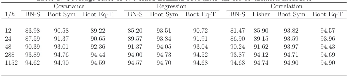
Table 2 shows that the superior performance of the bootstrap carries over to two-sided intervals. Symmetric intervals are generally better than equal-tailed intervals (which is consistent with the theory
based on Edgeworth expansions) and both improve upon the first order asymptotic theory. The gains
associated with the i.i.d. bootstrap can be quite substantial, especially for the smaller sample sizes,
when distortions of the BN-S intervals are larger. For instance, for the regression coefficient, the
coverage rate for a symmetric bootstrap interval when 1/h = 12 (cf. h = 1/48) is equal to 93.51%
(94.05%), whereas it is equal to 85.20% (91.37%) for the feasible asymptotic theory of BN-S (2004)
(the corresponding equal-tailed interval yields a coverage rate of 90.72% (93.04%), better than BN-S
(2004) but worse than the symmetric bootstrap interval). The gains are especially important for the
two-sided intervals for the correlation coefficient, when the asymptotic theory of BN-S (2004) does worst. For 1/h= 12, the bootstrap symmetric interval has a rate of 93.82% (the equal tailed interval
is in this case even better behaved, with a rate equal to 94.57%) whereas the BN-S interval based on
the raw statistic has a rate of 81.47% and the interval based on the Fisher-z transform has a rate of
85.90%. These numbers increase to 93.97%, 94.43%, 90.24%, and 91.62%, for the bootstrap symmetric
and equal-tailed intervals, the BN-S interval and the Fisher-z transform interval, respectively. For the
correlation coefficient, the bootstrap essentially removes all finite sample bias associated with the first
5
A detailed study of realized regressions
The realized regression estimator is one of the most popular measures of covariation between two assets. In this section we study in more detail the application of the i.i.d. bootstrap to realized regression.
We first provide a new interpretation for the feasible approach of BN-S (2004). In particular, we
establish a link between the standard Eicker-White heteroskedasticity robust variance estimator and
the variance estimator proposed by BN-S (2004). We then exploit the special structure of the regression
model to obtain the asymptotic distribution of the bootstrap realized regression estimator. We relate
the bootstrap variance with the Eicker-White robust variance estimator. We end this section with a
discussion of the second order accuracy of the i.i.d. bootstrap in this context.
5.1 The first order asymptotic theory revisited
Supposedp(t) = Θ (t)dW(t) where Θ is independent of W.1 Then, conditionally on Σ, we can write
yli =βlkiyki+ui, (5)
where independently acrossi= 1, . . . ,1/h,ui|yki ∼N(0, Vi),withVi ≡Γli−Γ
2
lki
Γki,andβlki≡
Γlki
Γki. Here
Γlki =
Rih
(i−1)hΣlk(u)du. Thus, the regression coefficient in the true DGP describing the relationship
between yli and yki is heterogeneous (it depends on i) and the true error term in this model is
heteroskedastic.
When we regressyli onyki to obtain ˆβlk, we get that ˆβlk P
→βlk≡ Γlk
Γk.Thus, ˆβlk does not estimate
βlkibut insteadβlk, which can be thought of as a weighted average ofβlki. We can write the underlying
regression model as follows:
yli =βlkyki+εi, (6)
whereεi = (βlki−βlk)yki+ui.It follows thatεi|yki ∼N((βlki−βlk)yki, Vi), independently across i.
Moreover, noting that E(yki) = 0,
Cov(yki, εi) =E(ykiεi) = (βlki−βlk) Γki = Γlki−βlkΓki,
which in general is not equal to zero (unless the volatility matrix is constant). However,EP1i=1/hykiεi
=
0, and therefore ˆβlk converges in probability toβlk. Because E(ykiεi)6= 0, ˆβlk does not consistently
estimateβlki but estimatesβlk instead. This is the parameter of interest, and therefore the
endogene-ity problem is not a concern here. Nevertheless, the fact that E(ykiεi)6= 0 and is heterogeneous has
important consequences for the asymptotic inference on βlk, as we now explain.
1We make the assumption of no leverage and no drift for notational simplicity and because this allows us to easily
To find the asymptotic distribution of ˆβlk, we can write
√ h−1βˆ
lk−βlk
=
√
h−1P1/h
i=1ykiεi
P1/h i=1y2ki
= (Γk)−1 √
h−1 1/h
X
i=1
ykiεi+oP (1).
The asymptotic variance of √h−1βˆ
lk is thus of the usual sandwich form Vβ ≡ V ar
√
h−1βˆ
lk
=
(Γk)−2B,where B = limh→0Bh, and Bh = V ar
√
h−1P1/h
i=1ykiεi
.Because E(ykiεi) 6= 0, we have
that
Bh=h−1
1/h
X
i=1
E yki2ε2i−h−1
1/h
X
i=1
(E(ykiεi))2≡B1h−B2h.
We can easily show that
B= lim
h→0Bh =
Z 1
0
Σ2lk(u) + Σl(u) Σk(u)−4βlkΣlk(u) Σk(u) + 2β2lkΣ2k(u)
du.
It follows that
Sβ,h≡ √
h−1(ˆβ
lk−βlk)
p
Vβ →
dN(0,1),
where Vβ = (Γk)−2B. We can contrast this result with Proposition 1 of BN-S (2004). It is easy to
check that B =g(lk),i, where g(lk),i is defined as in Proposition 1 of BN-S (2004) (where we let i= 1
here given that we measure the integrated regression coefficient over the [0,1] interval).
It is helpful to contrast the BN-S (2004) variance estimator of Vβ with the Eicker-White
het-eroskedasticity robust variance estimator that one would typically use in a cross section regression
context. Let ˆεi denote the OLS residual underlying the regression model (6). Then, the Eicker-White
robust variance estimator of B is given by ˆB1h =h−1P1i=1/hy2kiˆε2i.In contrast, noting that xβi=ykiˆεi,
BN-S (2004)’s estimator ofB corresponds to
h−1gˆβ =h−1
1/h
X
i=1
y2kiˆε2i −h−1
1/h−1
X
i=1
ykiˆεiyk,i+1ˆεi+1 ≡Bˆ1h−Bˆ2h. (7)
We can see thath−1ˆg
β = ˆB1h−Bˆ2h, where ˆB1his the usual Eicker-White robust variance estimator, and
ˆ
B2h =h−1Pi1=1/h−1ykiˆεiyk,i+1ˆεi+1. This extra term is needed to correct for the fact that E(ykiεi)6= 0
and is heterogeneous, as we noted above. In particular, ˆB1h →B1h and ˆB2h→B2h in probability.
5.2 First order asymptotic properties of the pairs bootstrap
The i.i.d. bootstrap applied to the vector of returns yi is equivalent to the so-called pairs bootstrap,
a popular bootstrap method in the context of cross section regression models. Freedman (1981)
proves the consistency of the pairs bootstrap for possibly heteroskedastic regression models when the
dimension p of the regressor vector is fixed. Mammen (1993) treats the case where p → ∞ as the sample size grows to infinity. Mammen (1993) also discusses the second order accuracy of the pairs
bootstrap is not only first order asymptotically valid under heteroskedasticity in the error term, but
it is also second-order correct.
For the bivariate case, the pairs bootstrap corresponds to resampling the pairs (yli, yki) in an i.i.d.
fashion. Although we focus on this case here, our results follow straightforwardly when dealing with
a multiple regression model where we regress the intraday returns on asset l on the returns of more
than one asset. In this case, the pairs bootstrap corresponds to an i.i.d. bootstrap on the tuples that
collect the dependent and all the explanatory variables.
Let ˆβ∗lk denote the OLS bootstrap estimator from the regression of yli∗ on yki∗. It is easy to check
that ˆβ∗lk converges in probability (underP∗) to ˆβ
lk =
P1/h
i=1E∗(yli∗y∗ki)
P1/h
i=1E∗(y∗ki2)
. The bootstrap analogue of the
regression error εi in model (6) is thus ε∗i = y∗li−βˆlky∗ki, whereas the bootstrap OLS residuals are
defined as ˆε∗i =yli∗ −βˆ∗lkyki∗.
Our next theorem provides the first order asymptotic properties of ˆβ∗lk.
Theorem 5.1 Suppose (1) holds. As h→0,
a) √h−1βˆ∗
lk−βˆlk
→d∗
N0, V∗
β
, in probability, where V∗
β =
ˆ Γk
−2
B∗
h.
b) B∗h=V ar∗√h−1P1/h
i=1y∗kiε∗i
=h−1P1i=1/hyki2ˆε2i ≡Bˆ1h.
c) V∗
β →P (Γk)−2B∗ 6=Vβ (except when the volatility matrix is constant), where B∗ =B+R01(Σlk(u)−βlkΣk(u))2du.
Part (a) of Theorem 5.1 states that the bootstrap OLS estimator has a first order asymptotic
normal distribution with mean zero and covariance matrix V∗
β. Its proof follows from Theorem 3.2.
Parts (b) and (c) show that the pairs bootstrap variance estimator is not consistent for Vβ in the
general context of stochastic volatility. One exception is when volatility is constant, in which case
B∗=B and V∗
β →P Vβ.
To understand the form ofV∗
β, note that we can write
√
h−1βˆ∗
lk−βˆlk
=
1/h
X
i=1
yki∗2
−1
√ h−1
1/h
X
i=1
yki∗ε∗i.
Since P1i=1/hyki∗2 →P∗ P1i=1/hyki2 = ˆΓk, in probability, it follows that
√
h−1βˆ∗
lk−βˆlk
=Γˆk
−1√
h−1 1/h
X
i=1
y∗kiε∗i +oP∗(1),
in probability. We can now apply a central limit theorem to √h−1P1/h
i=1yki∗ε∗i to obtain the limiting
normal distribution for √h−1βˆ∗
lk−βˆlk
. It follows that
√
h−1βˆ∗
lk−βˆlk
in probability, where Vβ∗ = Γˆk
−2
Bh∗, with Bh∗ = V ar∗√h−1P1/h
i=1y∗kiε∗i
. Part (b) of Theorem
5.1 follows easily from the properties of the i.i.d. bootstrap. In particular, we can show that Bh∗ =
h−1P1i=1/hy2kiˆε2i, since P1i=1/hykiˆεi = 0 by construction of ˆβlk. Thus, the i.i.d. bootstrap variance of
the scaled average of the bootstrap scores y∗
kiε∗i is equal to ˆB1h, the Eicker-White heteroskedasticity
robust variance estimator of the scaled average of the scoresykiεi.
Theorem 5.1 (part c) shows that the pairs bootstrap does not in general consistently estimate the
asymptotic variance of ˆβlk. An exception is when volatility is constant. This is in contrast with the
existing results in the cross section regression context, where the pairs bootstrap variance estimator
of the least squares estimator is robust to heteroskedasticity in the error term. This failure of the
pairs bootstrap to provide a consistent estimator of the variance of ˆβlk is related to the fact that, as
we explained in in the previous section, we cannot in general assume that E(ykiεi) = 0, unless for
instance when volatility is constant. When the scores have mean zero, i.e. E(ykiεi) = 0, the
Eicker-White robust variance estimator, and therefore the pairs bootstrap variance estimator, are consistent
estimators of the asymptotic variance of the scaled average of the scores. Both Freedman (1981)
and Mammen (1993) make this assumption. The fact that E(ykiεi) 6= 0 creates a bias term in ˆB1h,
which is estimated with the variance estimator proposed by BN-S (2004). Because B∗
h = ˆB1h, the
pairs bootstrap variance estimator is not a consistent estimator ofBh =V ar
√
h−1P1/h
i=1ykiεi
. The
heterogeneity (and non zero) mean property of the scores in our context is crucial to understanding
the differences between the realized regression and the usual cross section regression.
The i.i.d. bootstrap is nevertheless first order asymptotically valid when applied to thet-statistic
T∗
β,h (defined in (3)), as our Theorem 3.2 proves. This first order asymptotic validity occurs despite
the fact thatVβ∗ does not consistently estimateVβ.The key aspect is that we studentize the bootstrap
OLS estimator with ˆVβ∗ (defined in (4)), a consistent estimator of Vβ∗, implying that the asymptotic variance of the bootstrap t-statistic is one.
5.3 Second order asymptotic properties of the pairs bootstrap
In this section, we study the second order accuracy of the pairs bootstrap for realized regressions. In
particular, we compare the rates of convergence of the error of the bootstrap and the normal
approx-imation when estimating the distribution function of Tβ,h. This is accomplished via a comparison of
the Edgeworth expansion of the distribution ofTβ,hwith the bootstrap Edgeworth expansion ofTβ,h∗ ,
which we derive here. See Gon¸calves and Meddahi (2008) and Zhang et al. (2010) for two recent
papers that have used Edgeworth expansions for realized volatility as a means to improve upon the
first order asymptotic theory.
The results in this section are derived under the assumption of zero drift and no leverage (i.e.
W is assumed independent of Σ). As in Gon¸calves and Meddahi (2009), a nonzero drift changes the
expressions of the cumulants derived here. The no leverage assumption is mathematically convenient
Allowing for leverage is a difficult but promising extension of the results derived here.
Finally, we follow BNGJPS (2006) and assume that the spot covariance matrix Σ (t) = Θ (t) Θ′(t)
satisfies the following assumption
Σ (t) = Σ (0) +
Z t
0
a(u)du+
Z t
0
σ(u)dWu+
Z t
0
v(u)dZu, (8)
wherea,σ, andvare all adapted c`adl`ag processes, withaalso being predictable and locally bounded, and Z is a vector Brownian motion independent of W.
The second order asymptotic properties of the pairs bootstrap that we study in this section involves
the asymptotic distribution of statistics such as the realized cross-bipower variation of the log-price
process,p(t), t≥0, for powers larger than 2. The asymptotic distribution derived by BNGJPS (2006)
for such statistics is valid under Assumptions (1) and (8).
For i = 1,3, we denote by κi(Tβ,h) the first and third order cumulants of Tβ,h, respectively.
Conditionally on Σ, the second order Edgeworth expansion of the distribution ofTβ,his given by (see
e.g. Hall, 1992, p. 47),
P(Tβ,h≤x) = Φ (x) + √
hq(x)φ(x) +o√h,
where for any x ∈ R, Φ (x) and φ(x) denote the cumulative distribution function and the density
function of a standard normal random variable. The correction termq(x) is defined as
q(x) =−
κ1+1
6κ3 x
2
−1
,
where κ1 and κ3 are the coefficients of the leading terms of κ1(Tβ,h) and κ3(Tβ,h), respectively. In
particular, up to order O√h, ash→0,κ1(Tβ,h) = √
hκ1 and κ3(Tβ,h) = √
hκ3.
Given this Edgeworth expansion, the error (conditional on Σ) incurred by the normal
approxima-tion in estimating the distribuapproxima-tion of Tβ,h is given by
sup
x∈R|
P(Tβ,h≤x)−Φ (x)|= √
hsup
x∈R|
q(x)φ(x)|+O(h).
Thus, supx∈R|q(x)φ(x)|is the contribution of orderO√hto the normal error.
Similarly, we can write a one-term Edgeworth expansion for the conditional distribution ofT∗
β,has
follows
P∗(Tβ,h∗ ≤x) = Φ(x) +√hqh∗(x)φ(x) +OP(h),
where q∗
h is defined as
q∗h(x) =−(κ∗1,h+κ∗3,h(x2−1)/6),
and where κ∗
1,h and κ∗3,h are the leading terms of the first and the third order cumulants of Tβ,h∗ . In
particular,κ∗
1
T∗
β,h
=√hκ∗
1,h and κ∗3
T∗
β,h
=√hκ∗
3,h, up to order OP
√
h.
given by
P∗ Tβ,h∗ ≤x−P(Tβ,h≤x) = √
h (q∗h(x)−q(x))φ(x) +OP(h)
= √h(plimq∗h(x)−q(x))φ(x) +oP
√
h
= −√h
(κ∗1−κ1) +
1 6(κ
∗
3−κ3) x2−1
φ(x) +oP
√
h,
where κ∗1 ≡ plimκ1∗,h and κ∗3 ≡ plimκ3∗,h. If κ∗1 = κ1 and κ∗3 =κ3, P∗
Tβ,h∗ ≤x−P(Tβ,h≤x) =
oP√h,and the bootstrap error is of a smaller order of magnitude than the normal error which is
equal to O√h. If this is the case, the bootstrap is said to be second-order correct and to provide an asymptotic refinement over the standard normal approximation.
The following result gives the expressions of κi and κ∗i for i = 1,3. We need to introduce some
notation.
Let
A0 =
Z 1
0
Σk(u) Σlk(u)−βlkΣ2k(u)
du,
A1 =
Z 1
0
2Σ3lk(u) + 6Σl(u) Σlk(u) Σk(u)−18βlkΣ2lk(u) Σk(u) −6βlkΣ2
k(u) Σl(u) + 24β2lkΣlk(u) Σ2k(u)−8β3lkΣ3k(u)
du,
B =
Z 1
0
Σ2lk(u) + Σl(u) Σk(u)−4βlkΣlk(u) Σk(u) + 2β2lkΣ2k(u)
du,
H1 =
4A0
Γk √
B, and H2 =
A1
B3/2.
Similarly, let
B∗ = B+
Z 1
0
(Σlk(u)−βlkΣk(u))2du,
A∗
1 = A1+ 2
Z 1
0
(Σlk(u)−βlkΣk(u))3du,
H1∗ = 4A0 Γk
√
B∗, and H ∗
2 =
A∗
1
B∗3/2.
Theorem 5.2 Suppose (1) and (8) hold with α≡0 andW independent of Σ. Then, conditionally on
Σ, (a) κ1= 12(H1−H2) and κ3= 3H1−2H2; and κ∗1 = 34(H1∗−H2∗) and κ3∗= 32(3H1∗−2H2∗).
Theorem 5.2 shows that the cumulants ofT∗
β,handTβ,hdo not generally agree. Notice in particular
thatB 6=B∗contributes to this discrepancy. B here denotes the limiting variance of the scaled average
of the scores whereasB∗ denotes its bootstrap analogue. As we noted before, under general stochastic
volatility, the pairs bootstrap does not consistently estimate B and the bias term is exactly equal to the difference between B and B∗, i.e. B∗ −B = R1
0 (Σlk(u)−βlkΣk(u))2du = plimh→0B2h,
where B2h = h−1Pi1=1/h(E(ykiεi))2. An exception is when the volatility matrix is constant, where B2h = 0 and therefore B∗ = B. In this case, we also have that A∗1 =A1 = A0 = 0, implying that
expansion to orderO(h) to be able to discriminate the two approximations. In the general stochastic
volatility case, the pairs bootstrap error is of orderO√h, similar to the error incurred by the normal approximation.
The lack of second order refinements of the pairs bootstrap in the context of realized regressions
is in contrast with the results available in the bootstrap literature for standard regression models (see
Mammen (1993)). One explanation for this difference lies in the fact that E(ykiεi)6= 0, as we noted
above. This implies thatTβ,h must rely on a variance estimator that contains a bias correction term,
as proposed by BN-S (2004). Instead, in the bootstrap regression, E∗(yki∗ε∗i) =hP1i=1/hykiˆεi = 0, and
therefore there is no need for the bias correction proposed by BN-S (2004). This implies that the bootstrap t-statistic T∗
β,h is not of the same form as Tβ,h, relying on a bootstrap variance estimator
ˆ
V∗
β that depends on an Eicker-White type variance estimator ˆB1∗h.
6
Empirical application
A well documented empirical fact in finance is the time variability of bonds risk, as recently documented
by Viceira (2007) and Campbell, Sunderam and Viceira (2009) for the US market. As suggested by
the CAPM, the bond risk is often measured by its beta over the return on the market portfolio. With
a positive beta, bonds are considered as risky as the market while a bond with a negative beta could
be used to hedge the market risk.
Viceira (2007) studies the bond risk for the US market by considering the 3-month (monthly) rolling realized beta as measured by the ratio of the realized covariance of daily log-returns on bonds
and stocks and the realized volatility of the daily log-return on stocks over the same period. Following
the standard practice, the number of days in a month is normalized to 22 such that the 3-month
realized beta is computed considering sub-samples of 66 days. From July 1962 through December
2003, Viceira (2007) reports a strong variability of US bond CAPM betas, which may switch sign even
though the average over the full sample is positive. Nevertheless, in his analysis Viceira (2007) does
not discuss the precision of the realized betas as a measure of the actual covariation between bonds
and stock returns.
The aim of this section is to illustrate the usefulness of our approach as a method of inference for realized covariation measures in the context of measuring the time variation of bonds risk. We
consider both the US bonds market, as in Viceira (2007), and the UK bonds market.
Our data set includes the daily 7-to-10-year maturity government bond index for the US and the
UK markets as released by JP Morgan from January 2, 1986 through August 24, 2007. As a proxy
for the US and the UK market portfolio returns, we consider the log-return on the S&P500 and the
FTSE 100 indices, respectively. The S&P500 index is designed to measure performance of the broad
domestic economy through changes in the aggregate market value of 500 stocks representing all major
companies traded on the London Stock Exchange. The first two series have a shorter history and
therefore constrained the sample we consider in this study.
From the estimates presented in Table 3 (Appendix A), the full-sample beta for bonds in the US
is about 0.024, slightly smaller than the UK bond beta, which is about 0.030. Both the bootstrap and
the asymptotic theory based confidence intervals display support that the true values of the betas in
both countries are positive.
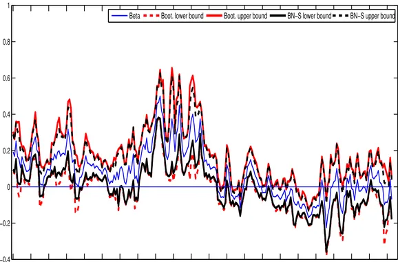
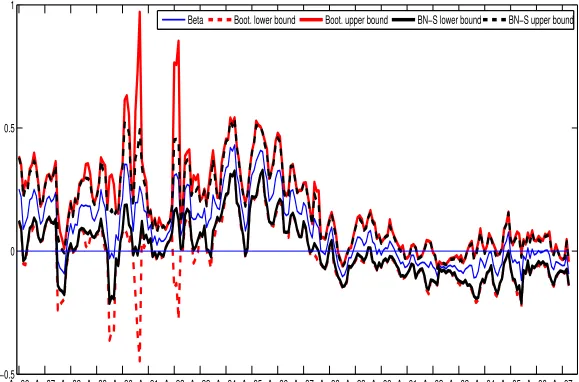
A closer analysis of Figures 1 and 2 shows that the average positivity of the betas hides considerable
time variation in both countries, a fact already documented by Viceira (2007) for the US market.
Furthermore, the betas for these two countries follow similar dynamics. We can distinguish two patterns for the 3-month betas. For the period before April 1997, the betas are mostly significantly
positive or, in few cases, non-significantly different from 0. This period is also characterized by betas
of larger magnitude, with a maximum value of 0.500 at the end of July 1994 for the US and 0.438 in
August 1994 for the UK. The period after April 1997 is characterized by a drop of the magnitude of
the bonds betas in both countries. They are often not significantly different from 0. For this whole
sub-period, the betas for the US and UK bonds are significantly negative only between June 2002
and July 2003, but in these cases their magnitude is small. We conclude that bonds are riskier in the
period before April 1997, while in the recent periods they appear to be non risky or at most a hedging
instrument against shocks on market portfolio returns.
A comparison of the bootstrap intervals with the intervals based on the asymptotic theory of BN-S
(2004) suggests that the two types of intervals tend to be similar, but there are instances where the bootstrap intervals are wider than the asymptotic theory-based intervals (see Tables 4 and 5 for a
detailed comparison of the two types of intervals for a selected set of dates). This is especially true for
the first part of the sample for the UK bond market, where the width of the bootstrap intervals can be
much larger than the width of the BN-S (2004) intervals. It turns out that these days correspond to
days on which there is evidence for jumps, as determined by applying the test for jumps of
Barndorff-Nielsen and Shephard (2006). Because none of the intervals discussed here (bootstrap or asymptotic
theory-based) are robust to the presence of jumps, a different analysis should be pursued for these
particular days.
7
Conclusion
This paper proposes bootstrap methods for inference on measures of multivariate volatility such as
integrated covariance, integrated correlation and integrated regression coefficients. We prove the first
order asymptotic validity of a particular bootstrap scheme, the i.i.d. bootstrap applied to the vector of
returns, for the three statistics of interest. Our simulation results show that the bootstrap outperforms
the feasible first order asymptotic approach of BN-S(2004).
bootstrap as proposed by Freedman (1981) and further studied by Mammen (1993). We analyze the
second order accuracy of this bootstrap method and conclude that it is not second order accurate.
This contrasts with the existing literature on the pairs bootstrap for cross section models, which
shows that this method is not only robust to heteroskedasticity in the error term but it is also second
order accurate. We provide a detailed analysis of the pairs bootstrap in the context of realized
regressions which allows us to highlight some key differences with respect to the usual application of
the pairs bootstrap in standard cross section regression models. These differences explain why the
pairs bootstrap does not provide second order refinements in this context.
An important assumption we make throughout this paper is that prices on different assets are observed synchronously and at regular time intervals. If prices are nonequidistant but synchronous,
results in Mykland and Zhang (2006) show that although the asymptotic conditional variance of the
realized covariation measures changes, the same variance estimators remain consistent. Consequently,
the same t statistics as those considered here can be used for inference purposes. In this case, we
can rely on the same i.i.d. bootstrap t statistics to approximate their distributions. The case of
non-synchronous data is much more challenging because in this case the realized covariation measures
are not consistent estimators of their integrated volatility measures. Different estimators (and
corre-sponding standard errors) are required. The extension of the bootstrap to these alternative estimators
and test statistics is left for future research.
Table 1. Coverage rates of one-sided nominal 95% intervals for covariation measures
Covariance Regression Correlation
Lower Upper Lower Upper Lower Upper
1/h BN-S Boot BN-S Boot BN-S Boot BN-S Boot BN-S Fisher Boot BN-S Fisher Boot
12 80.76 87.30 98.40 97.34 86.01 90.05 92.64 95.46 92.02 90.47 94.91 83.51 88.57 94.67 24 84.74 89.55 98.04 96.08 89.34 91.90 94.63 95.27 93.55 92.15 94.51 87.46 91.13 94.24 48 88.09 92.28 97.42 95.15 91.08 93.05 94.69 94.27 94.86 93.75 95.15 89.86 92.35 94.21 288 92.22 94.61 96.61 94.62 93.57 94.80 95.34 94.55 95.42 94.75 94.94 93.58 94.45 94.81 1152 93.69 94.98 95.50 94.39 94.30 95.07 95.35 94.78 95.27 94.92 95.03 94.38 94.82 94.95
Note: 10,000 replications, with 999 bootstrap replications each.
Table 2. Coverage rates of two-sided nominal 95% intervals for covariation measures
Covariance Regression Correlation
1/h BN-S Boot Sym Boot Eq-T BN-S Boot Sym Boot Eq-T BN-S Fisher Boot Sym Boot Eq-T
12 83.98 90.58 89.22 85.20 93.51 90.72 81.47 85.90 93.82 94.57 24 87.59 91.37 90.65 89.57 93.84 91.91 86.90 89.15 93.59 93.96 48 90.39 93.01 92.36 91.37 94.05 93.04 90.24 91.62 93.97 94.43 288 93.89 94.76 94.44 94.00 94.73 94.52 93.87 94.12 94.71 94.69 1152 94.62 94.90 94.59 94.57 94.70 94.68 94.63 94.74 94.90 94.90
Note: 10,000 replications, with 999 bootstrap replications each.
[image:21.792.103.689.271.399.2]Figure 1: Symmetric bootstrap and BN-S (2004) asymptotic theory based 95% two-sided confidence intervals for the CAPM 3-month (monthly) rolling realized beta of US bond. April 1986 through July 2007.
Apr86 Apr87 Apr88 Apr89 Apr90 Apr91 Apr92 Apr93 Apr94 Apr95 Apr96 Apr97 Apr98 Apr99 Apr00 Apr01 Apr02 Apr03 Apr04 Apr05 Apr06 Apr07 −0.4
−0.2 0 0.2 0.4 0.6 0.8 1
Beta Boot. lower bound Boot. upper bound BN−S lower bound BN−S upper bound
Figure 2: Symmetric bootstrap and BN-S (2004) asymptotic theory based 95% two-sided confidence intervals for the CAPM 3-month (monthly) rolling realized beta of UK bond. April 1986 through July 2007.
Apr86 Apr87 Apr88 Apr89 Apr90 Apr91 Apr92 Apr93 Apr94 Apr95 Apr96 Apr97 Apr98 Apr99 Apr00 Apr01 Apr02 Apr03 Apr04 Apr05 Apr06 Apr07 −0.5
0 0.5 1
Beta Boot. lower bound Boot. upper bound BN−S lower bound BN−S upper bound
Table 3. Full-sample estimates of bonds betas for the US and the UK
from January 2, 1986 through August 24, 2007 Beta BN-S 95% 2-sided CI Boot. symm. 95% CI US
0.024 [0.010,0.038] [0.009,0.038] UK
[image:24.612.111.499.92.667.2]0.030 [0.016,0.045] [0.015,0.046]
Table 4. Divergence between BN-S and bootstrap confidence intervals for the US
Date Beta BN-S Bootstrap
31-Jul-86 0.167 [0.027,0.306] [−0.022,0.355] 29-Aug-86 0.152 [0.015,0.289] [−0.053,0.357] 30-Sep-86 0.106 [0.017,0.194] [−0.041,0.252] 31-Jul-89 0.204 [0.036,0.371] [−0.025,0.432] 29-May-92 0.111 [0.004,0.217] [−0.010,0.231] 29-May-98 0.093 [0.001,0.184] [−0.012,0.197] 31-Aug-00 0.062 [0.002,0.121] [−0.002,0.126]
30-Jan-98 -0.054 [−0.101,−0.008] [−0.111,0.003] 27-Feb-98 -0.059 [−0.115,−0.002] [−0.128,0.010] 29-Dec-00 -0.055 [−0.109,−0.000] [−0.117,0.008] 31-May-01 -0.055 [−0.107,−0.004] [−0.113,0.003] 31-Dec-03 -0.154 [−0.302,−0.005] [−0.319,0.011] 29-Oct-04 -0.146 [−0.256,−0.036] [−0.293,0.001]
Table 5. Divergence between BN-S and bootstrap confidence intervals for the UK
Date Beta BN-S Bootstrap
31-Mar-88 0.070 [0.003,0.137] [−0.010,0.150] 31-Oct-90 0.197 [0.016,0.377] [−0.175,0.568] 31-Dec-90 0.262 [0.031,0.493] [−0.446,0.970] 30-Apr-92 0.307 [0.162,0.452] [−0.151,0.764] 29-May-92 0.314 [0.173,0.454] [−0.131,0.758] 30-Jun-92 0.288 [0.125,0.450] [−0.277,0.852] 29-Jan-93 0.129 [0.003,0.254] [−0.049,0.306] 26-Feb-93 0.131 [0.018,0.243] [−0.029,0.290] 31-Mar-93 0.153 [0.046,0.259] [−0.004,0.309] 31-Aug-93 0.122 [0.001,0.242] [−0.025,0.268] 29-Aug-97 0.054 [0.002,0.105] [−0.003,0.111] 30-Sep-97 0.132 [0.031,0.233] [−0.015,0.279] 31-Oct-97 0.109 [0.015,0.202] [−0.027,0.244]
Appendix B
This Appendix is divided in three parts. The first part (Appendix B.1) contains the proofs of Theorems 3.1, 3.2 and 5.1, as well as two auxiliary lemmas. The second part (Appendix B.2) contains the proof of Theorem 5.2 (a) and a list of lemmas useful for this proof. The third part (Appendix B.3) contains the proof of Theorem 5.2 (b) and a list of auxiliary lemmas.
Appendix B.1. Proofs of Theorems 3.1, 3.2 and 5.1.
Lemma B.1 Under (1), for any q1, q2 ≥ 0 such that q1 +q2 > 0, and for any k, l = 1, . . . , q,
h1−(q1+q2)/2P1/h
i=1|yli|q1|yki|q2 =OP(1).
Proof of Lemma B.1. Apply Theorem 2.1 of Barndorff-Nielsen, Graversen, Jacod, Podolskij and Shephard (2006) (henceforth BNGJPS (2006)).
Lemma B.2 Under (1), fork, l, k′, l′ = 1, . . . , q, with probability approaching one, (i)P1i=1/hy∗kiy∗liP→∗
P1/h
i=1ykiyli, and (ii) h−1
P1/h
i=1yki∗y∗liyk∗′iyl∗′i
P∗
→h−1P1/h
i=1ykiyliyk′iyl′i.
Proof of Lemma B.2. We show that the results hold in quadratic mean with respect toP∗, with probability approaching one. This ensures that the bootstrap convergence also holds in probability. For (i), we have
E∗
1/h
X
i=1
yki∗yli∗
=h−1E∗(yk∗1y∗l1) =h−1h
1/h
X
i=1
ykiyli=
1/h
X
i=1
ykiyli.
Similarly,
V ar∗
1/h
X
i=1
yki∗yli∗
=h−1V ar∗(y∗k1yl∗1) =h−1 E∗(yk∗1yl∗1)2−(E∗yk∗1yl∗1)2
=h−1
h
1/h
X
i=1
(ykiyli)2−
h
1/h
X
i=1
ykiyli
2 =
1/h
X
i=1
(ykiyli)2−h
1/h
X
i=1
ykiyli
2
=oP (1),
since Lemma B.1 implies thatP1i=1/h(ykiyli)2=OP(h) =oP(1) and Pi1=1/hykiyli =OP(1). The proof of
(ii) follows similarly and therefore we omit the details.
Proof of Theorem 3.1. (a) follows from Lemma B.2 by noting that the elements of x∗
ix∗′i are of all
of the formy∗
kiy∗liyk∗′iy∗l′i, fork, l, k′, l′ = 1, . . . , q. To prove (b), first note that both ˆV∗ and V∗ are non
singular in large samples with probability approaching one, ash→0. Second, letting
Sh∗ =V∗−1/2√h−1( 1/h
X
i=1
x∗i −
1/h
X
i=1
xi),
we have that
Th∗ = ˆV∗−1/2V∗1/2Sh∗.
Because ˆV∗−1V∗ P→∗ Iq(q+1)/2, in probability, the proof of (b) follows from showing that for any λ∈
Rq(q+1)/2 such that λ′λ= 1,
sup
x∈R|
P∗(
1/h
X
i=1
˜
where
˜
x∗i = λ′V∗λ−1/2√h−1λ′(x∗
i −E∗(x∗i)).
Clearly, E∗P1/h
i=1x˜∗i
= 0 andV ar∗P1/h
i=1x˜∗i
= 1. Thus, by Katz’s (1963) Berry-Essen Bound, for some small ǫ >0 and some constantK >0,
sup
x∈R P∗ 1/h X i=1 ˜
x∗i ≤x
−Φ(x) ≤K 1/h X i=1
E∗|x˜∗i|2+ǫ.
Next, we show that P1i=1/hE∗|x˜∗
i|2+ǫ=op(1). We have that
1/h
X
i=1
E∗|x˜∗i|2+ǫ = h−1E∗|x˜∗1|2+ǫ =h−1E∗
λ′V∗λ −1/2
h−1/2λ′(x1∗−E∗(x∗1))
2+ǫ
= h−1h−(2+ǫ)/2|λ′V∗λ|−(2+ǫ)/2E∗|λ′(x∗1−E∗(x∗1))|2+ǫ
≤ 22+ǫh−(2+ǫ/2)|λ′V∗λ|−(1+ǫ/2)E∗|λ′x∗1|2+ǫ ≤22+ǫh−(2+ǫ/2)|λ′V∗λ|−(1+ǫ/2)E∗|x∗1|2+ǫ
= 22+ǫh−1−ǫ/2|λ′V∗λ|−(1+ǫ/2)
1/h
X
i=1
|xi|2+ǫ,
where the first inequality follows from the Cr and the Jensen inequalities, and the second inequality
follows from the Cauchy-Schwarz inequality and the fact that λ′λ= 1. We let|z|= (z′z)1/2 for any vector z. It follows that
1/h
X
i=1
|xi|2+ǫ =
1/h
X
i=1
|xi|2(1+ǫ/2) ≤
1/h X i=1 q X j=1
yji2
2(1+ǫ/2)
.
Lemma B.1 and the Minkowski inequality imply thatP1i=1/h|xi|2+ǫ=OP(h1+ǫ), so thatP1i=1/hE∗|x˜∗i|2+ǫ =
OP(hǫ/2) =oP(1).
Proof of Theorem 3.2. SinceThconverges stably in distribution toN 0, Iq(q+1)/2
, by an application
of the delta method (see Podolskij and Vetter (2010, Proposition 2.5 (iii))),Tf,h d
→N(0,1). Similarly, by a mean value expansion, and conditionally on the original sample,
√
h−1f(vech(ˆΓ∗))−f(vech(ˆΓ))=√h−1∇′fvech(ˆΓ) vech(ˆΓ∗)−vech(ˆΓ)+o
P∗(1),
since ˆΓ∗→P∗ ˆ
Γ in probability. Let
Sf,h∗ ≡ √
h−1f(vech(ˆΓ∗))−f(vech(ˆΓ))
q
V∗
f
,
with V∗
f ≡ ∇′f(vech(ˆΓ))V∗∇f(vech(ˆΓ)). It follows that Sf,h∗ →d
∗
N(0,1) in probability, given
The-orem 3.1 (b). Next note that Tf,h∗ =
r V∗ f ˆ V∗ f
S∗f,h, where ˆVf∗ →P∗ Vf∗. The result follows from Polya’s
theorem (e.g. Serfling, 1980) given that the normal distribution is continuous.
Proof of Theorem 5.1. Take q = 2 and l= 1 and k= 2. Part (a) follows from Theorem 3.2 with
f(θ) = θ2/θ3. Vβ∗ and part (b) are proven in the text. Part (c) follows from Theorem 1 of BNGJS