http://dx.doi.org/10.4236/ti.2013.44026
A New Attribute Decision Making Model Based on
Attribute Importance
Wei Liu1, Yuming Zhai2*
1Glorious Sun School of Business and Management, Donghua University, Shanghai, China 2School of Economics and Management, Shanghai Institute of Technology, Shanghai, China
Email: [email protected], *[email protected]
Received September 2, 2013; revised October 2, 2013; accepted October 9, 2013
Copyright © 2013 Wei Liu, Yuming Zhai. This is an open access article distributed under the Creative Commons Attribution License, which permits unrestricted use, distribution, and reproduction in any medium, provided the original work is properly cited.
ABSTRACT
In the light of universality of uncertainty, we propose a decision making model in completed information system. Con- sidering the attribute reduction, attribute importance and mismatched information, a multiple attribute decision making model based on importance of attribute is constructed. First of all, decision table is obtained by the knowledge known and deleting reduced attributes. Also, attributes value reduction obtained to simplify the decision table and rules is ex- tracted. Then, rules are utilized to make decision for a new problem. Finally, an example is advanced to illustrate our model.
Keywords: Rough Set; Decision Making; Multiple Attribute
1. Introduction
Decision making is choosing a strategy among many dif- ferent projects in order to achieve some purposes. Ac- cording to various decision criteria, the decision-making problem is formulated as three different models: high risk decision, usual risk decision and low risk decision. With different attitude of decision makers for different types of decision models, decision criteria areformulated as five different models: optimistic-decisioncriterion, pessimis- tic-decision criterion, evenness-decision criterion, mini- mum-risk-decision criterion, compromise-decision crite- rion.
Rough set theory [1,2], a new mathematical approach to deal with inexact, uncertain or vague knowledge, has recently received wide attention on the research areas in both of the real-life applications and the theory itself. And the real-life applications speed up the theory re- search about rough set. Rough set theory is an extension of set theory, in which a subset of a universe is described by a pair of ordinary sets called the lower and upper ap- proximations. Rough set theory is emerging as a power- ful theory dealing with imperfect data. It is an expanding research area which stimulates explorations on both real- world applications and on the theory itself. It has found practical applications in many areas such as knowledge
discovery, machine learning, data analysis, approximate classification, conflict analysis, and so on. The theory of rough sets has been successfully applied to diverse areas, such as pattern recognition, artificial intelligent, machine learning, knowledge acquisition, economy forecast, data mining and so on [3,4]. Rough set theory adopts the con- cept of equivalence classes to partition the training in- stances according to some criteria. Two kinds of parti- tions are formed in the mining process: lower approxi- mations and upper approximations, from which certain and possible rules are easily derived. It operates only on the data and does not require any added information; it is completely data-driven.
tegrated the concept of rough inclusion relation into the Pawlak rough set model, thus being able to allow for some degree of misclassification in the mining process. Probabilistic rough set approximations can be formulated based on the notions of rough membership functions [11] and rough inclusion [12]. Also, rough set over dual-uni- verse is studied [13].
Since extended models introduction, they have been used in many research fields successfully. In these mod- els, decisions about new problems are made according rules extracted. However, some attributes of new prob- lems are inconsistent with rules completely. In this situa- tion, how to make decision might well repay investiga- tion.
In this paper, considering imperfectly matching be- tween new problem and rules exit, we introduce relative importance when deal with new problems. Firstly, we present same basic concept of rough set. Then we con- struct a new multiple attribute decision making model by considering relative importance of attribute. Finally, an example is advanced to illustrate our model.
2. Preliminaries
The rough set theory, firstly introduced by Pawlak in 1982, is a valuable mathematical tool for dealing with vagueness and uncertainty [10,11]. A rough set is a for- mal approximation of a crisp set (i.e., conventional set) in terms of a pair of sets which give the lower and the upper approximation of the original set.
Let I
U A,
be an information system (attribute-value system), where U is a non-empty set of finite ob- jects (the universe) and A is a non-empty, finite set of attributes such that for every . a is the set of values that attribute a may take. The informa- tion table assigns a value
: a
a UV aA V
a x from Va to each at-
tribute a and object x in the universe U. With any there is an associated equivalence relation IND(P):
PA
, 2 ,
IND P x y U a P a x a y (1)
The relation IND(P) is called a P-indiscernibility rela-tion. The partition of U is a family of all equivalence classes of IND(P) and is denoted by U IND P
(orU P). If
x y, IND P
, then x and y are indiscerni-ble (or indistinguishaindiscerni-ble) by attributes from P.Let X U be a target set that we wish to represent using attribute subset P; that is, we are told that an arbitrary set of objects X comprises a single class, and we wish to express this class (i.e., this subset) using the equivalence classes induced by attribute P.
However, the target set X can be approximated using only the information contained within P by constructing the P-lower and P-upper approximations of X:
P
,
P
PX x x X PX x x X (2)
The P-lower approximation, or positive region, is the union of all equivalence classes in
xP which arecon-tained by (i.e., are subsets of) the target set. The lower approximation is the complete set of objects in U P that can be positively (i.e., unambiguously) classified as belonging to target set X.
The P-upper approximation is the union of all equi- valence classes in
xP which have non-empty intersec-tion with the target set. The upper approximation is the complete set of objects that in U P that cannot be positively (i.e., unambiguously) classified as belonging to the complement (X) of the target set X. In other words, the upper approximation is the complete set of objects that are p.
In summary, the lower approximation of a target set is a conservative approximation consisting of only those objects which can positively be identified as members of the set. (These objects have no indiscernible “clones” which are excluded by the target set.) The upper approxi- mation is a liberal approximation which includes all ob- jects that might be members of target set. (Some objects in the upper approximation may not be members of the target set.) From the perspective of U P, the lower ap- proximation contains objects that are members of the target set with certainty (probability = 1), while the upper approximation contains objects that are members of the target set with non-zero probability (probability > 0).
An interesting question is whether there are attributes in the information system (attribute-value table) which are more important to the knowledge represented in the equivalence class structure than other attributes. Often, we wonder whether there is a subset of attributes which can, by itself, fully characterize the knowledge in the database; such an attribute set is called a reduct.
Formally, a reduct is a subset of attributes such that
REDP
1)
RED P
x x , that is, the equivalence classes in-
duced by the reduced attribute set RED are the same as the equivalence class structure induced by the full attrib- ute set P.
2) the attribute set RED is minimal, in the sense that
xRED a
x P for any attribute ; in otherwords, no attribute can be removed from set RED with-out changing the equivalence classes
aRED
xP.A reduct can be thought of as a sufficient set of fea- tures—sufficient, that is, to represent the category struc- ture.
tigation, and that will ultimately be of use in predictive modeling.
In rough set theory, the notion of dependency is de- fined very simply. Let us take two (disjoint) sets of at- tributes, set P and set Q, and inquire what degree of de- pendency obtains between them. Each attribute set in- duces an (indiscernibility) equivalence class structure, the equivalence classes induced by P given by
P
x , and
the equivalence classes induced by Q given by
xQ. Let
xQ
Q Q1, 2, ,QN
, where Qi is a given equivalence class from the equivalence-class structure induced by attribute set Q. Then, the dependency of at-tribute set Q on attribute set P, P
Q , is given by
1 1N i i P
PQ Q
U
(3)That is, for each equivalence class Qi in
xQ, we add up the size of its lower approximation by the attrib- utes in P, i.e., PQi. This approximation (as above, for arbitrary set X) is the number of objects which on attrib- ute set P can be positively identified as belonging to tar- get set Qi. Added across all equivalence classes in
xQ, the numerator above represents the total number of ob- jects which—based on attribute set P—can be positively categorized according to the classification induced by attributes Q. The dependency ratio therefore expresses the proportion (within the entire universe) of such classi- fiable objects. The dependency P “can be inter-preted as a proportion of such objects in the information system for which it suffices to know the values of attrib- utes in P to determine the values of attributes in Q”.
Q
Another, intuitive, way to consider dependency is to take the partition induced by Q as the target class C, and consider P as the attribute set we wish to use in order to “reconstruct” the target class C. If P can completely re- construct C, then Q depends totally upon P; if P results in a poor and perhaps a random reconstruction of C, then Q does not depend upon P at all.
Thus, this measure of dependency expresses the degree of functional (i.e., deterministic) dependency of attribute set Q on attribute set P; it is not symmetric. The rela- tionship of this notion of attribute dependency to more traditional information-theoretic (i.e., entropic) notions of attribute dependence has been discussed in a number of sources.
The dependency of attribute set Q on attribute set P also be named as the relative importance (with decision attribute d).
3. Decision Making Model
Multi-attribute decision making (MADM) provides a structured approach to decision making. MADM ap-
proach requires that the selection be made among deci- sion alternatives described by their attributes. It assumes that the problem has predetermined number of decision alternatives.
There are three generic types of MADM problems as follows:
1) Selection: Given a set of decision alternatives, the selection task involves finding the alternative (or alterna- tives) judged by the decision maker as the most satisfy- ing.
2) Sorting: It consists of assigning each alternative to one of the predefined criteria. Assignment is often based on relative differences of decision alternatives along a criterion.
3) Ranking: It involves establishing a preference pre- order on the set of decision alternatives. The pre-order represents a priority list of the alternatives.
All the three types of MADM problems have been re- searched by many universities and research institutes. However, most MADM models almost neglected uncer- tainty or missing values in decision alternatives, which are impact on selection, sorting and ranking.
Here we propose a MADM model to overcome above disadvantages. Selection, sorting and ranking of MADM problems are the same fundamental principles and they are just have different application. So we choose selec- tion of MADM problems as an example to illustrate how to deal with uncertainty or missing values in decision alternatives.
Let support that the decision making system is a com- plete information system. A complete information system means all decision rules can be found in the rule table. We consider mismatched values in decision alternatives and construct a new MADM model. The steps of deci- sion making are as follows.
Step 1: Obtain information table (information matrix) according to problems described.
Step 2: Obtain decision table from information table by computing weights and RED in rough set theory.
Step 3: Reduce attributes values to obtain clear deci- sion table.
Step 4: Extract decision rules and computer their con- fidence degree, coverage degree and support degree. Every rule denotes an alternative.
Step 5: Compare a new problem with alternatives and judge through confidence degree, coverage degree and support degree.
4. Example
Suppose Table 1 is an information system, which c1, c2, c3, c4, c5, c6, c7, c8 are conditional attributes and d is decisional attribute [14].
Table 1. Information system.
U c1 c2 c3 c4 c5 c6 c7 c8 d
1 15 4 5 239 34 4 6 7 d1
2 1 1 1 600 70 38 15 13 d1
3 6 0 3 145 13 3 1 4 d1
4 0 1 0 138 16 3 1 3 d1
5 0 0 0 580 90 25 6 12 d1
6 1 0 1 398 35 7 1 5 d1
7 2 1 6 125 3 1 0 1 d1
8 0 0 0 160 30 5 3 8 d1
9 1 1 1 50 60 5 3 2 d2 10 0 0 1 121 81 5 4 6 d2 11 0 0 0 120 78 3 1 5 d2 12 0 0 0 150 60 4 1 7 d2 13 0 0 0 35 43 3 1 6 d2 14 0 1 0 56 50 3 1 5 d2 15 0 0 0 30 48 4 1 5 d2 16 0 0 0 220 80 4 5 5 d2 17 0 40 4 60 1 4 5 1 d3 18 1 44 0 55 2 3 2 2 d3 19 5 30 9 52 1 2 1 1 d3 20 0 36 3 99 2 1 1 2 d3 21 2 40 3 59 9 3 4 3 d3 22 2 60 2 66 6 2 1 3 d3 23 10 70 6 67 4 6 10 1 d3
24 26 28 35 150 75 30 12 16 d4
25 10 25 30 120 65 14 10 5 d4
26 28 40 33 142 75 35 22 15 d4
27 20 29 23 200 60 34 25 16 d4
28 0 0 0 68 5 1 0 0 d5 29 0 0 0 62 6 0 0 0 d5 30 0 0 0 54 3 1 0 0 d5
Table 2. Discretization rule.
0 1 2 c1 [0, 10) [10, 20] (20, +∞)
c2 [0, 25) [25, 50] (50, +∞) c3 [0, 5) [5, 10] (10, +∞) c4 [0, 120) [120, 240] (240, +∞) c5 [0, 30) [30, 60] (60, +∞) c6 [0, 10) [10, 20] (20, +∞) c7 [0, 6) [6, 12] (12, +∞) c8 [0, 5) [5, 10] (10, +∞)
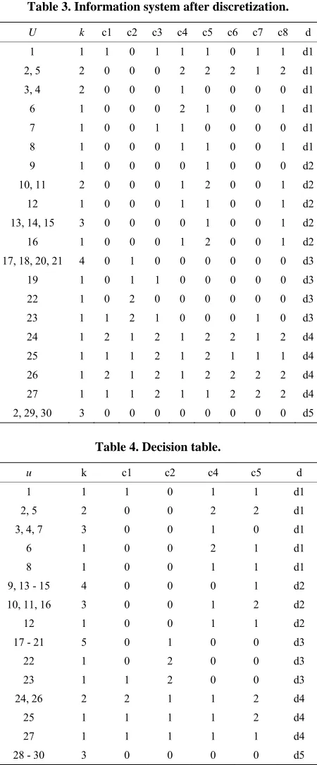
after discretization.
Table 4 is information system after reduction, which is named decision table.
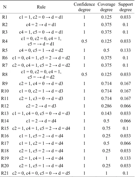
Table 5 is rules extracted from decision table.
Let support that the decision making system is a com- plete information system. A complete information system means all decision rules can be found in the rule table.
Table 3. Information system after discretization.
U k c1 c2 c3 c4 c5 c6 c7 c8 d
1 1 1 0 1 1 1 0 1 1 d1
2, 5 2 0 0 0 2 2 2 1 2 d1
3, 4 2 0 0 0 1 0 0 0 0 d1
6 1 0 0 0 2 1 0 0 1 d1
7 1 0 0 1 1 0 0 0 0 d1
8 1 0 0 0 1 1 0 0 1 d1
9 1 0 0 0 0 1 0 0 0 d2
10, 11 2 0 0 0 1 2 0 0 1 d2
12 1 0 0 0 1 1 0 0 1 d2
13, 14, 15 3 0 0 0 0 1 0 0 1 d2
16 1 0 0 0 1 2 0 0 1 d2
17, 18, 20, 21 4 0 1 0 0 0 0 0 0 d3
19 1 0 1 1 0 0 0 0 0 d3
22 1 0 2 0 0 0 0 0 0 d3
23 1 1 2 1 0 0 0 1 0 d3
24 1 2 1 2 1 2 2 1 2 d4
25 1 1 1 2 1 2 1 1 1 d4
26 1 2 1 2 1 2 2 2 2 d4
27 1 1 1 2 1 1 2 2 2 d4
2, 29, 30 3 0 0 0 0 0 0 0 0 d5
Table 4. Decision table.
u k c1 c2 c4 c5 d
1 1 1 0 1 1 d1
2, 5 2 0 0 2 2 d1
3, 4, 7 3 0 0 1 0 d1
6 1 0 0 2 1 d1 8 1 0 0 1 1 d1
9, 13 - 15 4 0 0 0 1 d2
10, 11, 16 3 0 0 1 2 d2
12 1 0 0 1 1 d2
17 - 21 5 0 1 0 0 d3
22 1 0 2 0 0 d3 23 1 1 2 0 0 d3
24, 26 2 2 1 1 2 d4
25 1 1 1 1 2 d4 27 1 1 1 1 1 d4
28 - 30 3 0 0 0 0 d5
In completed information system, confidence degree is a very important concept. Based on confidence degree, we know “c1 = 0, c2 = 0, c4 = 1, c5 = 1 → d = d1” and “C1 = 0, c2 = 0, c4 = 1, c5 = 1 → d = d2” are two ap-parently contradictory statements. “c1 = 0, c2 = 0, c4 = 1, c5 = 1 → d = d1” and “c1 = 0, c2 = 0, c4 = 1, c5 = 1 → d = d2” should be ignored.
[image:4.595.69.342.87.641.2]REFERENCES
Table 5. Rules.
N Rule Confidence degree Coverage degree Support degree
R1 c1 = 1, c2 = 0 → d = d1 1 0.125 0.033 R2 c4 = 2 → d = d1 1 0.375 0.1 R3 c4 = 1, c5 = 0 → d = d1 1 0.375 0.1 R4 c1 = 0, c2 = 0, c4 = 1, c5 = → d = d1 0.5 0.125 0.033 R5 c4 = 0, c5 = 1 → d = d2 1 0.5 0.133 R6 c1 = 0, c4 = 1, c5 = 2 → d = d2 1 0.375 0.1 R7 c2 = 0, c4 = 1, c5 = 2 → d = d2 1 0.375 0.1 R8 c1 = 0, c2 = 0, c4 = 1, c5 = → d = d2 0.5 0.125 0.033 R9 c2 = 1, c4 = 0 → d = d3 1 0.714 0.167 R10 c1 = 0, c2 = 1 → d = d3 1 0.714 0.167 R11 c2 = 1, c3 = 0 → d = d3 1 0.714 0.167 R12 c2 = 2 → d = d3 1 0.286 0.066 R13 c1 = 1, c4 = 0, c5 = 0 → d = d3 1 0.143 0.033 R14 c1 = 2 → d = d4 1 0.5 0.066 R15 c2 = 1, c4 = 1, c5 = 2 → d = d4 1 0.75 0.1 R16 c1 = 1, c5 = 2 → d = d4 1 0.25 0.033 R17 c1 = 1, c2 = 1 → d = d4 1 0.5 0.066 R18 c2 = 1, c5 = 2 → d = d4 1 0.25 0.033 R19 c2 = 1, c4 = 1 → d = d4 1 1 0.133 R20 c2 = 1, c5 = 1 → d = d4 1 0.25 0.033 R21 c2 = 0, c4 = 0, c5 = 0 → d = d5 1 1 0.1
[1] Z. Pawla, “Rough Sets,” International Journal of Interna- tional Sciences, Vol. 11, No. 5, 1982, pp. 341-356. [2] Z. Pawlak, “Rough Sets Theoretical Aspects of Reason-
ing about Data,” Kluwer Academic Publishers; Dordrecht, 1991.
[3] I. T. R. Yanto, P. Vitasari, T. Herawan, et al., “Applying Variable Precision Rough Set Model for Clustering Stu- dent Suffering Study’s Anxiety,” Expert Systems with Applications, Vol. 39, No. 1, 2012, pp. 452-459.
http://dx.doi.org/10.1016/j.eswa.2011.07.036
[4] S. Chakhar and I. Saad, “Dominance-Based Rough Set Approach for Groups in Multicriteria Classification Prob- lems,” Decision Support Systems, Vol. 54, No. 1, 2012, pp. 372-380. http://dx.doi.org/10.1016/j.dss.2012.05.050 [5] J. J. H. Liou and G. H. Tzeng, “A Dominance-Based
Rough Set Approach to Customer Behavior in the Airline Market,” Information Sciences, Vol. 180, No. 11, 2010, pp. 2230-2238.
http://dx.doi.org/10.1016/j.ins.2010.01.025
[6] S. K. Pal and A. Skowron, “Rough-Fuzzy Hybridization: A New Trend in Decision Making,” Springer-Verlag, New York, 1999.
[7] A. M. Radzikowska and E. E. Kerre, “A Comparative Study of Fuzzy Rough Sets,” Fuzzy Sets and Systems, Vol. 126, No. 2, 2002, pp. 137-155.
http://dx.doi.org/10.1016/S0165-0114(01)00032-X [8] W. Ziarko, “Probabilistic Rough Sets,” Rough Sets, Fuzzy
Sets, Data Mining, and Granular Computing, Vol. 3641, 2005, pp. 283-293.
http://dx.doi.org/10.1007/11548669_30 In recent papers, research commutations always due
with new problem using Table. All example are illustrate just comply with rules. For example, a new problem, “C1
= 1, c2 = 0”, compared with rules we know that d = d1. [9] W. Ziarko, “Variable Precision Rough Set Model,” Jour- nal of Computer and System Sciences, Vol. 46, No. 1, 1993, pp. 39-59.
http://dx.doi.org/10.1016/0022-0000(93)90048-2 If c1 = 1, c2 = 0 and c5 = 2, which decision should we
make? There is no rule abstract from decision table. Here, attribute importance is considered. For “c1 = 1, c2 = 0 and c3 = 2”, “c1 = 1, c2 = 0 → d = d1” and “c1 = 1, c5 = 2 → d = d4”, we just need compare the relative importance of c2 and c5.
[10] D. Slezak and W. Ziarko, “Bayesian Rough Set Model,” Proc. of the Int. Workshop on Foundation of Data Mining, Maebashi, 9 December 2002, pp. 131-135.
[11] J. Błaszczyński, R. Słowiński and M. Szeląg, “Sequential Covering Rule Induction Algorithm for Variable Consis- tency Rough Set Approaches,” Information Sciences, Vol. 181, No. 5, 2011, pp. 987-1002.
http://dx.doi.org/10.1016/j.ins.2010.10.030 From formula 3), we know c2a c5a.
So, follow with “c1 = 1, c2 = 0 → d = d1” and the de-cision is “c1 = 1, c2 = 0, c5 = 2 → d = d1”.
[12] X. Zhang, Z. Mo, F. Xiong, et al., “Comparative Study of Variable Precision Rough Set Model and Graded Rough Set Model,” International Journal of Approximate Rea- soning, Vol. 53, No. 1, 2012, pp. 104-116.
http://dx.doi.org/10.1016/j.ijar.2011.10.003
5. Conclusion
This paper provides a new multiple attribute decision making model. This model is special in utilizing rules extracted for new problems. By comparing new problems with rules extracted, both cases are considered. Com-pared with existing studies, this new model can handle problems which are not mismatched with every condition. We can utilize this model to deal with uncertainty or missing values in decision alternatives. This model can be used in marketing analysis, investment strategies and
anagement engineering.
[13] R. Yan, J. Zheng, J. Liu and Y. Zhai, “Research on the Model of Rough Set over Dual-Universes,” Knowledge- Based Systems, Vol. 23, No. 8, 2010, pp. 817-822. http://dx.doi.org/10.1016/j.knosys.2010.05.006
[14] G. Yang, X. Wu and Y. Song, “Multi-Sensor Information Fusion Fault Diagnosis Method Based on Rough set The- ory,” System Engineering and Electronics, Vol. 31, No. 8, 2009, pp. 2013-2019.