Absorption Capacity, Structural Similarity and Embodied Technology Spillovers in A ‘Macro’ Model: An Implementation within a CGE Framework

Munich Personal RePEc Archive

Absorption Capacity, Structural

Similarity and Embodied Technology

Spillovers in A ‘Macro’ Model: An

Implementation within a CGE

Framework

Das, Gouranga and Powell, Alan A. L.

University of Florida, Gainesville, USA, Monash University,

Melbourne, Clayton Campus, Australia

1 January 2000

Absorption Capacity, Structural Similarity and Embodied

Technology Spillovers in A ‘Macro’ Model: An Implementation

within a Computable General Equilibrium Framework

Gouranga G. Das

a

and Alan A. Powell

b

Abstract

In this paper, all technology transfers are embodied in trade flows within a

three-region, one-traded-commodity version of the GTAP model. Exogenous Hicks-Neutral

technical progress in one region can have uneven impacts on productivity elsewhere.

Why? Destination regions’ ability to harness new technology depends on their

absorptive capacity

and the

structural congruence

of the source and destination.

Together with trade volume, these two factors determine the recipient’s

spillover

coefficient

(which measures its success in capturing foreign technology). Armington

competition between the outputs of the three economies and shifts in their terms of

trade loom large in the general equilibrium adjustment.

JEL Classification

: D58, F1, O3.

Key Words

: Absorption Capacity, Capture Parameter, Trade, Technology Spillover,

and CGE.

a

Post-Doctoral Research Fellow, School of Forest Resources and Conservation/ Institute of Food and Agricultural Sciences, University of Florida, PO Box 110 410, Gainesville, FL 32611-0410. USA,

Contact Telephone No: [1] 352 846 0877 (Office), Fax No: [1] 352 846 1277, E-mail:

[email protected](Corresponding Author).

b

1. Introduction

Thelinksbetweeninternationaltrade,growthandinventionarewell-establishedinthe

literature. Manylessdevelopedcountries(LDCs)havepursuedliberaltradeandtechnology

policiesandhavereliedontechnologiesoriginatingintheindustrialised,developedcountries

(DCs) of the world. Giventhat the latest state-of-the-art isresearched anddeveloped in the

DCs, we address the problem of “effective assimilation” and “absorption” of advanced

technologyintheLDCs.

There is evidence that knowledge spills over from the sources of innovation to the

destinations through different channels. Two principal channels through which such

transmission of advanced knowledge-capital occurs are (a) International Trade in goods and

services and (b) Foreign Direct Investment (of which Joint-Ventures are special case). The

literature has highlighted the role of trade in technology spillovers from North to South [Coe,

Helpman and Hoffmaister 1995 & 1997), Connolly (1997), Keller (1997), Edwards (1997),

Hall and Jones (1998), Padoan (1996)]. This paper is about “embodied” spillovers of

knowledge through international trade in commodities. Technology transferred via bilateral

trade in goods embodying technological advances leads to enhancement of productivity in the

receiving countries. Here, we consider the effects of ‘Absorptive Capacity (AC)’ and

‘Structural Similarity (SS)’ in fostering technology acquisition. Among the plethora of

papers on the determinants of technological innovation, the bulk has been in the context of

DCs. The paper by Hans van Meijl and Frank van Tongeren (April, 1997) (henceforth,

referred to as MT) is a stepping stone for modelling issues of technology transfer from the

countries at the frontiers of technology creation to the relatively laggard recipient countries

within the global applied general equilibrium model, GTAP2F

1

. It is argued that “local” or

domestic usability of the foreign technology depends on the destination’s capacity to identify,

procure and use the diffused state-of-the-art.

We implement the ‘embodied’ knowledge spillovers in a highly aggregated version

of the GTAP model—that is, a one-traded-commodity, three-region version of GTAP.3F

2

GTAP, like many CGE models, adopts Armington’s (1969) treatment of commodity

substitution, so that even if all regions produce the same generic commodity, the substitution

elasticity between that commodity produced in region A and the “same” commodity

produced in region B, is not infinite. Thus, even in a one-commodity version of GTAP the

‘Law of One Price’ does not hold. Working at the one-commodity level has the advantage of

concentrating on inter-regional competition in the goods market without having to deal with

the large amount of detail entailed in keeping track also of inter-generic commodity

substitution.

We aggregate the GTAP database to one-commodity and three-region (USA, EU, and

ROW) database. The generic commodity that is traded internationally will be called “Stuff”.

Each region produces one tradable good (its own type of “Stuff”) and one non-tradable (its

own Capital Goods). It is necessary to include a non-tradable in each region because GTAP

specifies that capital formation is supplied completely by a domestic industry which does not

export. Note, however, that the domestic capital goods industry in any country merely

assembles a bundle of traded goods (which include foreign tradables). Consumers absorb

Stuff produced at home, as well as the two imported varieties. We consider a Hicks-Neutral

general total factor productivity (TFP) shock in the “Stuff” sector originating in one of the

three regions, viz. the USA. Such a TFP shock is general output-augmenting by nature. Its

impact on productivity in the destinations via an embodiment index, an absorption capacity

index, and a structural similarity index, are studied. Section 2 and 3 describe the theoretical

premise and the database corresponding to our aggregation respectively. Section 4 documents

the GTAP implementation, the closure and the perturbation introduced into the system.

2. Theoretical Premise

2.1 Embodied Spillover Hypothesis

3

Growth and development of the LDCs depend not only on the extent and nature of

the foreign technology which is available to them via participation in international trade in

goods and services, but also on their capabilities for effectively absorbing the diffused

state-of-the-art. Current state-of-the-art technologies created by concerted research efforts are

embodied in the commodities produced using the newly created ‘ideas’. The

knowledge-capital generated at the sources of inventions, spills over to the destinations through bilateral

trade linkages. This is the “embodiment hypothesis”: technical knowledge flows through

traded goods. Note that the creation (as distinct from the transmission) of knowledge-capital

is beyond the scope of this model.

The adaptability and local usability of the diffused technologies depends on the

Absorptive Capacity [Cohen and Levinthal5F

4

(1990)] of the destinations and the Structural

Similarity [Hayami and Ruttan (1985)] between the trading nations. In the literature, the

importance of ‘SS’ has been discussed especially in the context of agriculture. Here in a

single-sector model with one trading sector per region, this focus is not valid. However, the

maximum potential for productivity enhancement attainable with a given stock of ideas can

be achieved only if both AC and SS are high.6F

5

Productivity growth rates of countries are related through international trade linkages

and associated “embodied” knowledge-spillovers. In their model, AC is constructed as a

binary (source- and destination-specific) index of human-capital-induced absorption capacity

of Country A vis-a-vis Country B. They also use a binary index for SS. It is based on the

3

Our approach is more modest than the approach by Eaton and Kortum (1994, 1996a & b) [henceforth, EK], Grossman and Helpman (1991a & b), Jones (1995). All of these dynamic general equilibrium models have considered the possible interlinkages between invention, technology diffusion, growth and productivity. Eaton and Kortum have developed an empirical dynamic general equilibrium model of technology-diffusion based on a “quality-ladder” approach. Better quality inputs embodying the latest ‘ideas’ always replace the ‘state-of-the-art’ currently in practice.

4 _{To the best of our knowledge, the role of such factors in assimilating the foreign technology was first} emphasised in the literarure by Cohen and Levinthal. Based on their notion of absorption capacity and its importance, some authors like Keller (1997), Nelson (1990), to name a few, have extended the discussion initiated by them.

similarity of factor proportions in the two regions (but unlike AC, SS is symmetric). These

two indexes conjointly determine the ‘productive efficiency’ parameter for effective

assimilation of the technology by the recipient countries.7F

6

Our model differs in several details. Firstly, we restrict ourselves to a one-sector

(‘tradable’ Stuff) technology for production. ‘Stuff’ is produced in a world divided into three

regions. Like “ectoplasm” in the one sector Neo-Classical growth model, ‘Stuff’ is easily

transmutable from consumable to investment goods. Second, unlike MT where AC is a binary

index involving both ‘source’ and ‘destination’, we make the ‘AC’ factor destination-specific

only. The ‘SS’ factor retains its ‘binary’ affix, though. Third, as will become evident below,

we have modified MT’s ‘embodied spillover function’.

It is argued that domestic usability of the transmitted foreign technology depends

mainly on the recipient’s capability to identify, procure and utilise the diffused technology.

This simplification reflects our desire to keep the model simple by concentrating on

first-order effects. It seems likely that if region ‘C’ is good at absorbing technology from region

‘A’, it will be equally good at absorbing technology from another region ‘B’ which (from C’s

point of view) is structurally similar to ‘A’. Thus, the AC factor is made destination-specific

only (unlike in MT where they carry both source and destination affixes). The basic spillover

equations are rationalised in the next section.

2.2 Production Technology and Spillover Function

2.2a Production Technology

The production technology tree in the GTAP model uses a nested production

function. Here we specialize the notation for use with the one-traded-commodity version.

At the top level, a composite outputY_r is produced in region ‘r’ with a Leontief fixed

proportion technology using intermediate inputs Qr. and a primary input composite Q V

r.. Qr.

is intermediate input demand for Armington composite “stuff” by any region ‘r’. Each Q_r. is

produced in a CES production nest using domestic stuff and a composite of foreign ‘stuff’

distinguished by country of origin (using the Armington assumption). Thus, we can write the

CES production function for the intermediate input nest as

Q_r.= A_r {δDr(Qrr) -β

r. _+(1-δD r)(Q

F r)

-β

r.}-1/βr. _(2.1a)

where ‘r’ is the region using the domestically sourced tradable stuff Q_rr and the foreign inputs

composite of stuff QFr. δ D

r is

the distribution parameter (positive constant). βr.≠-1 is the

substitution parameter. The superscripts ‘D’ and ‘F’ are used to identify domestic and

foreign components respectively. The substitution elasticity between domestic and foreign

stuff is [1/(1+βr.)].

For notational convenience, in Q_rs the first subscript refers to the using region and the

second one refers to the foreign source of Stuff. For example, let the three regions in our

implementation be A, B and C so that r,s∈{A, B, C}. Then, if r=C is the ‘using’ region, and

s=B or A, Q_rr=Q_CC is the domestically sourced ‘stuff’ in C while Q_CA and Q_CB are Stuff

imported by C from B and A respectively.

QFr is produced in region ‘r’ using the Stuff imported from other regions, say, ‘s’ and

‘t’. Let Q_rs and Q_{rt be respectively the intermediate input demand for Stuff from ‘s’ and ‘t’ by}

using region ‘r’. This leads us to write the CES production nest for QFr as below:

QFr = A F

r {δ F

r(Qrs) -β

rF _+(1-δF r)(Qrt)

-β

rF }-1/βrF (2.1b)

where s,t≠r; s≠t. δF_r is the distribution parameter associated with this production nest. The

elasticity of substitution in ‘r’ between imported stuffs is [1/(1+β_rF)]. If β_r.=β_rF, (2.1b) is

equivalent to writing Q_r. as a CES function in ‘stuff’ from all three sources.

Primary factor composite QVr is produced combining the primary factors land (T),

labor (L), and capital (K). Qfr is the demand for primary factor‘f’ in region ‘r’ where f∈{L,

QVr = A V

r {

δ

f

∑

rf (Q f r)

-ρ

r_}-1/ρr _(2.2)

where δV_rf’s are distribution parameters (positive constants) (with

δ

f

∑

rf =1, ∀r) and ρr is

the substitution parameter. The substitution elasticity between primary factors in region ‘r’ is

[1/(1+ρr)]. In the above equations, Ar, A F

r and A V

r are technical progress parameters.

Q_r. and QVr are combined using a fixed proportion technology with no scope for

substitution between intermediate inputs and the primary factors. However, as seen above,

there is scope for substitution between domestic and imported varieties of Stuff, as there is

between L, K and T. At the top level the (Leontief) production function is:

Y_r=[AO]_r min {AOrQr. , Q V

r} (2.3)

where Y_r is the flow of final output and AOr is an intermediate input augmenting technical

change parameter. [AO]_r is the Hicks-Neutral Technical Progress (HNTP) parameter.

2.2b Spillover Equation and Productivity Shock

The spillover hypothesis (as documented in Section 2.1 above) is captured by a

technology-transmission equation incorporating destination-specific AC and source- and

destination-specific SS. Exports from source ‘r’ to destination ‘s’ determine an

“Embodiment index’’ E_rs. The latter, together with ACs and SSrs determine the value of a

“Spillover Coefficient” γ_s(E_rs, AC_s, SS_rs) via the spillover function γ_s.

The details of this chain are now explained, starting at the top. Note that there is

only one source of ‘exogenous’ technological improvement in the current treatment, so that

‘r’ is unique.8F

7

Stuff produced using the improved technology embodies this technological

improvement. Exports of ‘Stuff’ from ‘r’ to the trade partners ‘s’ transmit these embodied

technological advances but do not necessarily lead to enhancement of productivity in the

define an “Embodiment Index” E_{rs (where}

0

≤

E

≤

1

of embodied knowledge received via bilateral trade linkages between ‘r’ and ‘s’ so that

E_rs= X_rs/Y_{s (2.4)}

where X_{rs is the bilateral exports of Stuff from source ‘r’ to the clients ‘s’ and Y}s is the

domestic production of Stuff in ‘s’. E_rs , thus, measures the amount of embodied knowledge

obtained via bilateral exports from ‘r’ to ‘s’ per unit of output of Stuff produced in client ‘s’.9F

8

The recipient-specific AC-index AC_s (where 0

≤

≤

index SSrs (where 0

≤

≤

the efficiency with which the knowledge embodied in bilateral trade flows from source ‘r’ is

captured by the recipients ‘s’ :

θ_s=AC_s.SS_rs (2.5)

The realised productivity level from the potential streams of latest technology is dependent

on θ_s∈[0,1] with θ_s=1 implying full realisation of the foreign technology-induced

productivity improvement. θ_s and E_rs jointly determine the value of the ‘Spillover

Coefficient’γ_s(E_rs, θ_s) for the destination ‘s’. γ_s(.) is a strictly concave function of E_rs with the

properties that

γ_s(0) =0, γ_s(1) =1,

γ

′ =

γ

′′

s = −θs(1−θs)/Ers 1+θs

<0.

where primes indicate the first (′) and the second (′′) derivatives with respect to E_{rs. We}

consider an exogenous TFP improvement in the technology for producing “stuff” in region

‘r’. Specifically, the shock is a Hicks-neutral improvement in the productivity of each

primary factor there. Figure 1 shows the way in which technological knowledge embodied in

trade flows affects the spillover of productivity from a source to a destination region.

Figure 1: Flowchart for the transmission mechanism in the model.

The improvement in productive efficiency leads to value-added augmenting technical

change in ‘Stuff’. Hence, AV_r in the value-added nest of the production tree [see equation

(2.2)] is the appropriate technological change parameter for considering HNTP. In GTAP

notation, this is AVA(r). The transmission equation showing how the productivity

improvement in ‘r’ affects productivity in ‘s’ is as follows:

ava(s) = γ_s(E_rs, θs). ava(r) (2.6)

where ava(s) and ava(r) are respectively the percentage improvements in the productivity

‘levels’ (HNTP parameters, AVA) in the value-added nest of the production function of

regions ‘r’ and ‘s’ (the convention in the GTAP-system of notation being that the lower case

variables represent the percentage-changes in the corresponding ‘level’ variables). This

transmitted improvement is higher, the higher are the values of AC_s and SS_rs.

More specifically,

γ

(

E

θ

)

E

s

Given the functional form,

γ

(

E

,

θ

)

≤

E

≤

1

0

<

θ

<

1

,

0

≤

E

≤

1

∂γ

∂θ θ γ

′

= − − + < s

s

rs s

E s_{[1 ln ] 0.} ∂γ

∂θ ′

< s s

0 implies that marginal returns of γ_s to E_rs are a

decreasing function of θ_s . It can also be shown that

∂γ

∂θ

s

= [–γ_s(E

rs).lnErs] >0 and

∂ γ

∂θ

= [ (lnErs) 2

.Ers 1−θ

s

]>0 i.e., γs is a convex function of θs.

Thus, the γ_s function shows increasing marginal returns to θs.10F

9

Substitution of (2.7) into (2.6) shows that, all told, the equation governing the

technological spillover is given by

ava(s)=E_rs1-ACs.SSrs .ava(r) (2.8)

Substitution of (2.4) into equation (2.8) yields the fundamental spillover equation for

implementation in GTAP as

ava(s) = [X_rs/Y_s]1−AC SSs. rs

.ava(r) (2.8a)

Being ‘neutral’ in nature, the exogenous HNTP shock uniformly reduces the input

requirements associated with producing a given level of output of Stuff.

3.The GTAP Database and Aggregation

The aggregation procedure involves working in several steps with necessary

computer files for performing the task. All these files are documented in details in the

Appendix. The MODHAR programme available in the Windows version [WINGEM] of

GEMPACK (General Equilibrium Modelling Package) was run interactively to create a

HAR (Header ARray) file named SET1BY3.HAR from a text file (SET1BY3.TXT) defining

the elements of the sets. We refer to our one-traded-commodity, three-region model as

1×3GTAP. The aggregated database comprising trade, production and input-output data was

produced by running Mark Horridge’s programme “DAGG” on the 3×3GTAP bilateral and

input-output data in Version 3 of the database. The procedure is described in details in the

Appendix.

9 _{With the determinants AC and SS of θ}

The additional parameters introduced in the parameter file are HK(s) and SS(r, s).

HK(s) represents AC_{s as described in Section 2. Their values are set arbitrarily.} Assuming

that the EU is more ‘similar’ to the US in both SS and AC than to the ROW, higher values

are assigned for these exogenous variables in case of EU as compared to ROW; that is, AC_EU

> AC_{ROW and SSEU,US > SSROW,US}. The Appendix documents them as appended in the TABLO

file.

4.GTAP Implementation

5.2

Additional Equation

The economic model is the one described in Hertel (ed.) [1997] with an additional

behavioural equation, two new parameters and two new coefficients, plus some additional

national accounting identities coded by Philip D. Adams.

Equation (2.8a) in the notation of the GTAP-system of equations is:

ava(i,s)= [VXWD(i,r,s)/VOW(i,s)](1-ACs.SSrs) _{. ava(i,r) (2.8b)}

where i ∈ TRAD_COMM. TRAD_COMM contains traded commodity ‘Stuff’ only,

VXWD(i,r,s) is the value of exports of tradable commodity ‘i’ from ‘r’ to ‘s’ evaluated at

world ‘fob’ prices [i.e., X_{rs in equation (2.8a)]; VOW (i,s) is the value of output of tradable}

commodity ‘i’ in ‘s’ evaluated at world ‘fob’ prices [i.e., Y_s in (2.8a)]. The model is encoded

in TABLO language for GEMPACK software as reported in the Appendix. In our

implementation, we define one region at a time as the source of invention—set named ‘SRC’.

The countries other than the source belong to the set named ‘REG_NOT_SRC’. These two

equation only (i.e., equation (2.8b)) in TABLO11F

10

language.

TABLE 1: Key Technology Spillover Equation in the TABLO Source file

Equation MOD_EMB_SPLOVER

!This equation gives the Embodied Spillovers via Trade in the recepients!

(all, i, TRAD_COMM) (all, r, SRC) (all, s, REG_NOT_SRC)

ava(i,s)=[(VXWD(i,r,s)/VOW(i,s))^(1-HK(s)*SS(r,s))]*ava(i,r); (2.8b′)

The Appendix documents the changes made in the GTAP96.TAB by defining some additional

coefficients, variables and necessary equations.

5.2

Closure and Shock

All savers face a common price, PSAVE (which is the numeraire in the standard

closure of the model), for the savings commodity. The allocation of savings commodity

depends on the specification of the closure. Here it is assumed that the aggregate capital

stock is exogenous in all regions and that regional and global nett investment move together.

While no reallocation of regional shares in global investment is permitted, inter-industry

capital mobility within a region is allowed. This is known as the medium-run, or partial

long-run equilibrium standard closure in the GTAP literature. In all standard closures of

GTAP, the regional labor endowments are exogenous, while in the current closure new

investment does not add to the capital stock available in the solution period12F

11

. Hence the

productive capacities of all regions are unaffected in the period to which the simulation

results apply. However, as investment is a component of final demand, it affects economic

activity in the solution period via its impact on the demand. In the case of our 1×3 macro

aggregation of GTAP, these compositional influences are limited to the sourcing of “Stuff”

from different regions in the assembly of locally-specific capital goods.

Below we consider an arbitrary 2% TFP shock in the USA in the “Stuff” sector. In

the closure used here, prices, quantities of all non-endowment commodities, and regional

10 _{TABLO is an algebraic language for writing economic models and for defining the associated sets, equations,} coefficients, and variables for subsequent solution specifically compatible with the GEMPACK software suite (see Harrison and Pearson, 1996).

incomes are endogenous, while policy variables, other technical change variables, and

population [POP(r)] are exogenous to the model.

5. Analysis of Simulation Results

5.1 Macroeconomic Effects in Each Region

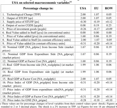
Table 2 summarises the impact of the perturbation on the macro variables.

TABLE 2 Simulated regional effects of technological change in the USA on selected macroeconomic variables(a)

Percentage change in: USA EU ROW

1. Technological Change [TFP] 2.00 1.07 0.05

2. Output of STUFF [qo] 2.00 1.07 0.05

3. Supply priceof STUFF [ps] -0.30 -0.19 +0.12

4. Output of sector CGDS [qcgds] 0.08 0.19 0.25

5. Price of investment goods [pcgds] -0.26 -0.17 +0.09 6. Real Value-added in Stuff [qva] (in conventional units) 0.00 0.00 0.00 7. Price of Value-added [pva] (in conventional units) 1.68 0.86 0.19 8. Real Value-added in Stuff [in constant efficiency units] 2.00 1.07 0.05 9. Price of Value-added [in constant efficiency units] -0.31 -0.20 +0.14 10. Nominal GDP [NA_gdpinc] from Income Side (market

prices)

1.67 0.86 0.19

11. Nominal GDP from Expenditure Side [NA_gdpexp] (market prices)

1.67 0.86 0.19

12. Nominal GDP at Factor Cost [NA_gdpfc] 1.68 0.86 0.19 13. Real GDP from Income side [NA_realgdpinc] (at market

prices)

1.99 1.06 0.06

14. Real GDP from Expenditure side [qgdp] (at market prices)

1.99 1.06 0.06

15. Real GDP at Factor Cost [NA_realgdpfc] 2.00 1.07 0.05 16. Price Index of GDP [NA_prigdpin] from Income side

(market prices)

-0.31 -0.20 +0.14

17. Price index of GDP from expenditure side[NA_prigdp] (market prices)

-0.31 -0.20 +0.14

18. Price Index of GDP at Factor Cost [NA_prigdpfc] (a) -0.31 -0.20 +0.14

19. Price index for GNE [NA_prigne] -0.28 -0.18 +0.10

(a) These values are for percentage changes of level variables from their control values (post- shock). Figures are rounded to 2 or 3 decimal places. The shock is a 2% increase in TFP. (a) Figures for row 18 are obtained by modifying the existing equation for it in GTAP National Accounts module and incorporating into it the ‘Tec_Chg’ variable as documented in the Appendix. These are the same as figures in row 9 after this adjustment has been made.

With fixed supplies of land, labor and capital and no factor-bias, a 2% TFP-shock in

‘Stuff’ in the USA leads to an increase in output in that sector and real GDP at factor cost of

exactly 2%. After the HNTP shock, we effectively have 2-percent more of each factor after

input-composite value-added measured in terms of constant efficiency units applicable in the

base-period. Hence, there has been no change in the usage of primary factors of production (as

measured in conventional units) between the base case and the shocked solution. This leads

to a zero percentage change in value-added (not quality adjusted) by factors of production

[row 6, Table 2]. However, real value-added (measured in constant efficiency units) increases

in all three regions.

The increase in productive efficiency of the ‘raw’ primary composite input

(measured in conventional units) leads to an increase in its marginal productivity (MP)—i.e.,

2.00, 1.07, and 0.05 per cent for USA, EU and ROW respectively 13F

12

. Since factors are paid

according to their marginal products, these increases in MP lead to increases in the price of

value-added and their constituents in all three regions. Being neutral in nature, this TFP

improvement causes equal percentage increases in the real rewards of all primary factors

within any given region.

We observe that there has not been full transmission of technical change from the

source to the destinations–EU and ROW. Table 3 suggests that the value of the spillover

coefficient depends more strongly on θ_s than on E_rs alone. Thus, whilst trade is the prime

vehicle for transmission of knowledge-flows, ACs and SSrs (and hence, θ_s ) are critical for

‘effective’ transmission of technology from ‘r’ to ‘s’. This is supported by the fact that even

when Ers has lower values, the magnification of them by θ_s can lead to a high rate of capture

of the technological improvement. Thus, EU with higher values of both AC_s and SS_rs, does

better than ROW at capturing the TFP improvement occurring in the USA despite ROW

12

The percentage changes in marginal (physical) productivities can be verified from computed GTAP variables as follows. In the levels, the value of the MPs of factors should equal their prices:

Pstuff * MPf = Pf (where f∈{L, K, T})

We have computed GTAP results for the percentage changes in Pstuff and in each Pf—pstuff, pL, pK, and pT (say)— in each region. Then, for example, we can use the above relationship to compute the percentage change in the marginal physical product of labour by:

% change in MPL= ({[Pf (initial) * (1+pf/100)] / [Pstuff (initial) * (1+pstuff/100)]}-1)*100 = 100* [{(pf/100)-(pstuff/100)}/(1+pstuff/100)]

having a higher value of E_rs. Consequently, in Table 2 we see a greater improvement in

technology in EU (1.07) as compared to that in ROW (0.05).

TABLE 3 Values of embodiment-index, spillover coefficient and capture-parameter (a)

GTAP Regions

Embodiment Index (E_rs)

Spillover Coefficient (γ_s)

Capture-Parameter (θ_s)

EU 0.014 0.540 0.855

ROW 0.020 0.023 0.030

USA 1.000 1.000 1.000

(a) Values shown relate to the pre-shock situation.

Stuff being the only sector whose production involves value-added, its share in total

value-added is unity in all three regions. As the TFP improvements cause real value-added

by factors of production (quality adjusted) to increase by the same percentages, the

percentage change in real GDP at factor cost in each region is equal to the respective TFP

shock (see rows 1 and 8, Table 2). Also, the price indexes for value-added in ‘Stuff’ (row 9

of Table 2) and for GDP at factor cost (row 18) are identical. Changes in real nett indirect

taxes (which are of fairly small magnitude) account for the wedges between real GDP at

market prices and real GDP at factor cost.

Now, the recorded NA_gdpfc (row 12, Table 2) is calculated on the basis of price

and quantity indexes of value-added measured in conventional units [pva]. These are taken

as given from the GTAP results. As the real value-added measured in constant efficiency

units (i.e., ‘quality-adjusted’) increases in all regions by the same percentage as the TFP

improvement, the effective price of value-added has to adjust accordingly so that the nominal

value-added measured in constant efficiency units matches the GTAP results. The increases

in real value-added (measured in constant efficiency units) of about 2 and 1 percent

respectively in USA and EU lead to falls in the corresponding price indices of about 0.3 and

attendant general equilibrium effects (to be discussed below)—in fact, it rises (0.14 per cent)

there.

5.2

Inter-regional Competition Effects

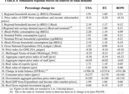
Table 4 shows that, region by region, there have been increases in nominal regional

household income [y(r)] and its uses ( rows 1, 7, 5 and 4).

TABLE 4 Simulated regional effects on sources of final demand(a)

Percentage change in: USA EU ROW

1. Regional household income [y (REG)] (Nominal) 1.91 1.00 0.21 2. Price index of GDP from expenditure and income sides(market

prices)

-0.31 -0.20 +0.14

3. Regional household income [u (REG) ] (Real) 2.19 1.17 0.12

4.Regional nett savings demand [qsave] (Real and nominal) (b) 1.91 1.00 0.21

5. (Real) Public consumption [ug (REG)] 2.20 1.19 0.09

6. Nominal Public consumption [yg(r)] 1.91 1.00 0.21

7. Nominal Private household expenditure [yp(REG)] 1.91 1.00 0.21 8. (Real) Private household consumption [up (REG)] 2.19 1.18 0.10 9. Gross National Expenditure (NA_realgne ] (Real) 1.92 0.99 0.14

10. Price index for GNE [NA_prigne] -0.28 -0.18 +0.10

11. McDougal Terms-of-trade (McDougal_TOT) -0.35 -0.21 +0.17

12. Aggregate export price index of stuff [pxw] -0.30 -0.19 +0.12 13. Aggregate import price index of stuff [piw] +0.05 +0.02 -0.05

14. Real value of exports [qxw] 1.71 1.19 0.05

15. Real value of imports [qiw] 1.01 0.50 0.46

16. Change in trade balance [DTBAL] (c) +1508.26 +3233.6 -4741.86

17. Consumer price index [ppriv] -0.277 -0.179 +0.104

18. Government aggregate purchase price index [pgov] -0.285 -0.189 +0.110 19. Real GDP from Expenditure and Income sides (market prices) 1.99 1.06 0.06

20. Real Gross regional investment [qcgds] 0.08 0.19 0.25

(a) Figures in this table are rounded to 2 or, 3 decimal places.

(b) This is the same in ‘nominal’ terms as there has been no %-change in its price PSAVE.

(c) Since the trade balance can pass through zero, percentage changes are avoided in the case of this variable. The change reported here is an ordinary change (million US $) changes of level values.

We first explain post-shock differential impacts on nominal income [y(r) ] which is

the sum of primary factor payments and receipts from various transactions taxes nett of

depreciation. Table 5 breaks up the component-wise effects on y(r). Earlier discussion shows

that the HNTP shock increases ‘pva’ and its components (row 7, Table 2). The increase in

y(r) has primarily been caused by the uniform increases in primary factor payments in all

TABLE 5 Simulated effects on nominal regional income(a)

Percentage change in: USA EU ROW

1. Nominal Regional Household income [y(REG)] 1.908 1.000 0.206

2. Contribution of Endowment income [pfac] 1.721 0.936 0.193

3. Contribution of Physical Depreciation 0.000 0.000 0.000

4. Contribution of pcgds to cost of replacing depreciated capital (nominal changes)

+0.031 +0.024 -0.013

5. Contribution of Output tax revenues 0.143 0.004 0.011

(a) Figures in this table are rounded to 3 or, 4 decimal places. Figures in row 1, when rounded to 2 decimal places, yield the same figures as in row 1 of Table 4. We do not report here the figures for all component-wise effects from tax receipts. Figures of very small magnitude (< 0.00003) are excluded.

We now turn to the discussion of impacts on sources of various income-uses.

5.2.a Region-wide impact on sources of final demands

In GTAP, each region’s demands for private expenditure [PRIVEXP (r)], public

expenditure [GOVEXP (r)] and saving [SAVE (r)] are determined by maximisation of a per

capita Cobb-Douglas utility function subject to the constraint that these three items totally

exhaust the regional income [INCOME(r)]. Under this specification, their fixed shares of

income result in the equality of percentage increases in nominal demand for the income uses

with the percentage increases in total nominal income.

Given the equality of percentage changes in the nominal variables14F

13

PRIVEXP and

GOVEXP in each region, we observe that the corresponding real variables in each region

move together but not strictly in proportion to each other (see rows 5 and 7, Table 4). The

changes in real consumption expenditures are attributed to the differential impacts of

movements in pgov (the aggregate government purchase price index) and ppriv (the

consumer price index or, CPI)—the divergence being caused by the diverse purchase patterns

of the private and public ‘households’15F

14

. Back-of-the-envelope calculation shows that

changes up(r) and ug (r) are almost exactly the differences between percentage changes in

nominal PRIVEXP and GOVEXP (rows 6 and 7, Table 4) and ppriv and pgov respectively

13 _{In terms of the TABLO file, strictly speaking, PRIVEXP and GOVEXP are coefficients which are equal to the} levels values of the variables ‘yp’ and ‘yg’. The latter one is added in the original TABLO file for computational conveniences.

(rows 17 and 18, Table 4).

The percentage increases in real private and public consumption demand for

composite Stuff are larger than the corresponding increases in domestic supply in every

region (rows 5 and 8, Table 4 and row 2, Table 2). In spite of the small percentage

increments in the market price of composite imports in USA (0.05) and EU (0.02), this leads

to increases in private household import demands of 1.35 and 0.7% in USA and EU

respectively16F

15

. The much larger fall in the price of domestically sourced Stuff—0.3 percent

in USA and 0.19 percent in EU—causes the relative price of domestic- vis-a-vis

foreign-sourced Stuff to fall by 0.35 and 0.21 percent in USA and EU respectively. Given the

expansionary effect on demand (qp) for composite Stuff due to the general increase in

consumption demand, this leads to substitution in favour of domestic ‘Stuff’ in USA and EU

and reinforces the expansion effect. This is reflected in increases of 2.2 and 1.2 per cent in

private consumption demand for domestic Stuff in USA and EU respectively.

As opposed to this, in the case of ROW, a decline in the price of composite imports

by 0.05 percent and a rise of 0.12 percent in the price of domestic Stuff causes the relative

price of domestic Stuff to increase by 0.17 percent. This leads to substitution in favour of

imported stuff with a relatively larger percentage increase (0.5) in demand for foreign

composite Stuff as compared to that in domestic stuff (0.07). Since Armington elasticities are

the same across uses and regions, similar considerations apply in the case of public

consumption. The aggregate utility index [u(r) ] proxies regional real income. In the model,

percentage changes in the sub-utility indexes for the public [ug(r)] and private [up(r)]

household consumption are equal to the percentage changes in real quantities purchased by

the representative government and private households respectively. The Cobb-Douglas utility

function is self-dual17F

16

as it generates a unit cost function of the same functional form as the

primal. Following this property, the income deflator [incdeflator(r)] for y(r) is defined as the

sum over the products obtained by multiplying the Cobb-Douglas price indexes for each

income use viz., ppriv(r), pgov(r) and psave with their corresponding region-wise shares in

total income18F

17

. Table 6 reports the values of the shares—i.e., PRIVEXP/INCOME,

GOVEXP/INCOME, SAVE/INCOME and the incdefaltor(r). Row 4 in Table 6 shows that

incdeflator(r) preserves the same ranking, sign and order of magnitude as the ppriv and pgov

(rows 17 and 18, Table 4). Subtracting row 4 of Table 6 from row 1 of Table 4, we

reproduce, almost exactly, the results on realincome (row 3, Table 4).

TABLE 6 Budget shares of each income use category and incdeflator (a)

Values of: USA EU ROW

1. PRIVEXP/INCOME 0.7711 0.7017 0.6926

2. GOVEXP/INCOME 0.2108 0.2158 0.1515

3. QSAVE/INCOME 0.0181 0.0825 0.1559

4. incdeflator -0.27 -0.17 +0.09

(a) The shares are calculated from base-period data and hence these are base-case values; under the Cobb-Douglas specification, these are unchanging parameters.

Now, the GDP deflator (pgdp) is weighted sum of percentage changes in the index of the

price of the domestic absorption (NA_prigne), in the export price index (pxw), in the price

index for exports to the international transportation sector (pm) and in the aggregate import

price index (pim)—the weights being the shares in GDP of gross national expenditure

(GNE), of exports (VXWD), of sales to the global transport sector (VST), and of imports

16 _{The duality between production and cost function is formally analogous to the duality between utility and} expenditure function—this implies that minimization of total outlay on public and private consumption and saving subject to the specified level of utility will give the same demand equations for these income uses. For a discussion on ‘self-duality’ between Cobb-Douglas production and cost function, see Varian (1984) Microeconomic Analysis, 2nd edition, pp. 62-64, and 69-73.

17 _{The mathematical expression for incdeflator (r) is:}

(VIWS)19F

18

. pgdp includes the change in the price of exportable Stuff (pxw) with a positive

weight that includes exports rather than just domestic consumption—as in the case of

NA_prigne. Also, pgdp includes ‘pim’ with a negative weight. Hence, the percentage

increase ‘pim’ and the percentage fall ‘pxw’ lead to a more negative change in pgdp than

NA_prigne. Now, the consumption deflators include the price of imports with positive

weight. These consumption deflators are included in NA_prigne and thus, it includes the

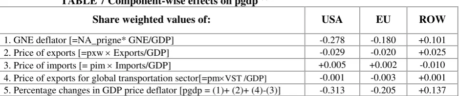
import price index with a positive weight.

TABLE 7 Component-wise effects on pgdp (a)

Share weighted values of: USA EU ROW

1. GNE deflator [=NA_prigne* GNE/GDP] -0.278 -0.180 +0.101

2. Price of exports [=pxw × Exports/GDP] -0.029 -0.020 +0.025

3. Price of imports [= pim × Imports/GDP] +0.005 +0.002 -0.010

4. Price of exports for global transportation sector[=pm×VST /GDP] -0.001 -0.003 +0.001 5. Percentage changes in GDP price deflator [pgdp = (1)+ (2)+ (4)-(3)] -0.313 -0.205 +0.137

(a) Calculated from base-period data. Figures in row 5 match the figures in row 2 in Table 4 when we do ‘rounding’ to 2 decimal places.

From Table 7, it is evident that the difference between pgdp and NA_prigne clearly

relates to the percentage deviation of the terms-of-trade (TOT) from the control scenario20F

19

.

The fall in TOT in USA and EU does not cause CPI, pgov and hence, NA_prigne to fall as

much as pgdp—see rows 1 and 5 in Table 7. This implies that a decline in TOT implies a

rise in the consumption deflators (which include price of imports) relative to pgdp (which

includes price of exports) in these regions.

18 _{The GDP deflator, pgdp, can be broken down into the following components as below:} pgdp= NA_prigne*(GNE/GDP)+ pxw*(VXWD/GDP)+ pm*(VST/GDP)—pim*(VIWS/GDP)

It is to be noted that ‘pm’ and ‘pxw’ are the same. Nominal domestic absorption, GNE(r) is expressed as: GNE(r)= PRIVEXP(r)+GOVEXP(r)+REGINV(r). Thus, the GNE deflator is:

NA_prigne (r)= ppriv (r)∗ [PRIVEXP(r)/GNE (r)] + pgov (r)∗[GOVEXP(r)/GNE (r)] + pcgds (r)∗ [REGINV (r)/GNE (r)]

19 _{After some algebraic manipulation, we can re-write the expression in Footnote 18 as:}

pgdp−NA_prigne=[pxw*{(VXWD+VST)/GNE}]−[pim*(VIWS/GNE)]−pgdp*(TradeBalance/GNE)] In the case of balanced trade, VXWD+VST=VXW=VIWS, this equation becomes:

pgdp−NA_prigne = (VIWS/GNE) (pxw − pim). Also, in case of balanced trade, GNE (r)=GDP (r). Thus, multiplying both sides of the above expression by [GNE/GDP], we re-write it as:

pgdp−NA_prigne = [pxw−pim]∗[VIWS/GDP] = [VXW/GDP] ∗ [pxw−pim]

Similar considerations explain relatively larger percentage changes in pgdp relative to

NA_prigne and the consumption deflators in case of ROW. We now elaborate the trade

competition in the wake of relative price divergences.

5.2.b Regional composition of International Trade

Due to the Armington specification of commodity substitution, even in a world with

one generic traded-commodity in every region, the relative price divergences (between the

three varieties of Stuff) across regions (after the TFP shock) induce changes in regional TOT

and open up the scope for inter-regional competition via trade. Consequently, these lead to

changes in the regional composition of exports and imports depending, inter alia, on the

movements in TOT. Looking at the global economy as a whole, we observe that after the

shock there has been an increase in the quantity index of global merchandise exports and

imports of Armington substitutable Stuffs by 0.57%21F

20

. However, ROW experiences a small

percentage rise in the price of domestically produced Stuff as compared to relatively large

percentage falls in the prices of Stuff exported by USA and EU (as explained in subsections

5.1 and 5.2.a). Thus, the price index of global merchandise exports of Stuff [pxwcom(Stuff)]

falls by 0.02%.22F

21

Similar considerations explain the percentage fall in the index of world

prices of total supplies of Stuff [pw (Stuff)].23F

22

Decomposition of region-specific differential TOT effects identifies the forces

behind such changes. We follow the decomposition à la McDougall (1993)24F

23

where the

percentage change in regional terms of trade [tot (r)] is split into two components as below:

tot(r) = px (•, r ) − pm (•, r ) (5.2.1)

20 _{The calculation involves multiplying region-wise shares of exports of Stuff in aggregate worldwide exports (at}

fob prices) by the corresponding percentage increases in regional aggregate volume of exports of Stuff and summation over the products thus obtained. ROW has a higher share (62 percent) in total world exports of Stuff than USA (17 percent) and EU (21 percent). Thus, 0.57 = (1.71×0.17)+(1.19×0.21)+ (0.05 × 0.62). 21 _{This is calculated as: (0.17 × -0.30) + (0.21 × -0.19) + (0.62 × 0.12) ].The price index of world trade [pxwwld]}

falls by 0.02 percent as well (similar calculations are involved).

22 _{The base-case shares of value of output of Stuff of each region at world prices (}

where px (•, r ) is the percentage change in the price received for exports and pm (•, r ) is the

percentage change in the price paid for imports. Suppose pxw (i, r) and piw (i, r) are

respectively the percentage changes of the export and import prices of traded commodity ‘i’

in any region ‘r’, and EXP_SHR (i, r) and IMP_SHR (i, r) are respectively the export share of

commodity ‘i’ in total export expenditure and import share of commodity ‘i’ in total import

expenditure in any region ‘r’. Thus,

px (•, r ) =A

∑

i

EXP_SHR(i, r) pxw(i,E r)EA (5.2.2a)

and

pm (•, r ) = A

∑

i

IMP_SHR(i, r) piw(i,E r)EA (5.2.2b)

Then the above expression for region r’s terms of trade can be written as:

tot(r) = A

∑

i

EXP_SHR(i, r) pxw(i,E r)EA − A

∑

i

IMP_SHR(i, r) piw(i,E r)EA

With further manipulation following McDougall (1993), this expression yields:

tot(r) = A

∑

i

(EXP_SHR(i, r) - IMP_SHR(i,E r)) (pw(i) -pxwwld)EA

+A

∑

i

EXP_SHR(i, r) (pxw(i,E r) -pw(i))E

− A

∑

i

IMP_SHR(i, r) (piw(i,E r) -pw(i))EA (5.2.3)

where pw(i) is the world price index for total supplies of good ‘i’ and pxwwld is the price

index of world trade (average of world prices of merchandise exports). The first term on the

right of (5.2.3), Wpe, captures the world price effect, whilst the last two terms show the

export price effect (Xpe) and the import price effect (Mpe) respectively.

‘Wpe’ shows that if the world price of commodity ‘i’ falls/rises relative to the

average of all world commodity prices [i.e., pw(i )≠pxwwld ], then, depending on the sign of

the regional nett trade share of good ‘i’, the direction of movement of regional TOT will be

determined. If ‘r’ is a nett exporter of ‘i’, and the world price of ‘i’ in general (i.e., averaged

over the sources) inflates relative to all prices, then, ceteris paribus, this is good for region

‘Xpe’ shows that if in any region, the exporters’ price of good ‘i’ falls relative to the

world price of ‘i’ [i.e., pw (i) ≠pxw (i, r) ], then TOT will deteriorate. Besides the size of the

shock, the extent of changes in such relativities [measured by (pxw (i, r) − pw (i))] reflect the

degree of product diversification in the market for ‘i’ (à la Armington assumption). With

low Armington elasticities, ceteris paribus, the spread between the two prices will tend to be

larger. By contrast, with a very large substitution elasticity, the absolute difference between

pxw(i, r) and pw(i) tends to be smaller so that they are almost equal. If there is erosion of

competitiveness following a shock, the large Armington elasticity coupled with the loss in

competitive edge can lead to big loss of export shares of a region and consequently, can have

adverse effect on TOT. That is, there may be a large fall in EXP_SHR(i,r) − IMP_SHR(i,r)

between the base case and the post-shock solution.

‘Mpe’ captures the effect of divergences [ piw(i, r) − pw(i) ]between the

region-specific import price of good ‘i’ and the world price of ‘i’ :it shows that if the latter rises

more than the former, then TOT will improve if there are no offsetting changes in ‘Wpe’ and

‘Xpe’.

In a one-traded-commodity world, since EXP_SHR (Stuff, r) is identical to IMP_SHR

(Stuff, r) and both are equal to unity, the first term on the right of Equation (5.2.3) for tot (r)

vanishes, so that this expression simplifies to the following:

tot(r) = pxw(stuff, r) − piw(stuff, r) (5.2.4)

Thus, in Table 8, ‘Wpe’ is zero across all regions. The intuition behind this result is

that ‘Wpe’ is meant to capture inter-generic-commodity competition, of which there is none

in this one-commodity version of GTAP. Since the share of Stuff in every region’s exports is

unity, ‘Xpe’ shows in its entirety the effect of changes in the export supply price of Stuff in a

region relative to an index of the average world price of Stuff. Analogously, ‘Mpe’ totally

TABLE 8 Decomposition of percentage changes in regional TOT(a)

GTAP Region

World price effect (Wpe)

(1)

Export price effect (Xpe) (2)

Import price effect (Mpe) (3)

Total TOT effect [tot(r)]

(4)= (1)+(2)−(3)

USA 0.00 -0.23 +0.12 -0.35

EU 0.00 -0.12 +0.09 -0.21

ROW 0.00 +0.18 +0.01 +0.17

(a) We have rounded percentage changes to 2 decimal places.

Table 8 shows that in all three regions, ‘Xpe’ is the most important source of the

change in TOT. The changes in regional export volumes can be ascribed to two-fold

movements: along the export demand schedule and shifts of the demand curve.

As the individual regions as exporters of Stuff face downward sloping foreign

demand curves for their region-specific Stuffs, a fall in the price of exports in USA and EU

(as opposed to a rise in the case of ROW) is consistent with percentage rises in exports from

USA and EU which are larger than the percentage expansion of exports from ROW to both of

these regions—see row 14 in Table 4. In part, this has been caused by the movements along

the export demand curve governed by the changes in price relativities between regions. Now,

the expansion in activity level (i.e., increase in regional aggregate import demand) in each

region results in outward shifts of the regional export demand curves. These changed trading

conditions entail allocation of demand for aggregate composite imports of Stuff by a region

across different sources of imports depending on relative price changes. Given the

expansionary effect on demand for all imports of Stuff [qim (stuff,r) ] by any region ‘r’ due to

the increase in intermediate input demand for it by firms producing Stuff and CGDS as well

as that in final demand by the public and private sectors (explained before in subsection

5.2.a), changes in relativities between the price of imported Stuff from any source ‘k’ (pms

(stuff,k,r)) and the aggregate import price index (pim (stuff, r)) confronting ‘r’ determine

changes in source-specific import demand by any region.

As products are differentiated by origin, divergences between the export prices for

Stuff produced in any region and the average world price for Stuff have given rise to changes

‘s’ and ‘k’, given the Armington elasticity, the expansionary effect on aggregate imports of

stuff (qim (stuff, r)) and the import share of ‘k’ in aggregate imports of ‘r’, then import of

Stuff from ‘s’ to ‘r’ [qxs (i,s,r) ] depends on the changes in relativities between the price of

imports of stuff from ‘k’ vis-a-vis that from ‘s’25F

24

. We discuss the change in composition of

bilateral export sales which is contingent on these shock-induced relative price effects.

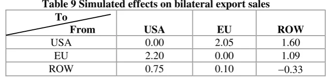
Aggregate imports into the USA increase by 1.0108 percent. In USA, the market

shares of EU and ROW in aggregate imports of tradable Stuff are 18 and 82 percent

respectively. A relatively large decline (0.183%) in the price of imported Stuff from EU to

USA as compared to a rise (0.104%) in case of imports from ROW to USA causes a 2.2

percent increase in imports of Stuff in USA from EU, whereas imports from ROW to USA

rise by 0.75 percent only. Given identical Armington elasticities across all regions (all equal

to 5), this translates into an increase in demand for Stuff from EU even though initially EU

has a lower export share in USA than ROW.

In the case of EU, aggregate imports increase by 0.4951 per cent, while the market

shares of USA and ROW in total imports are 20 and 80 percents respectively. The decline in

‘pms’ for USA (0.29%) as opposed to an increase (0.1%) in case of ROW translates into a

relatively larger increase of exports from USA (2.1%) to EU than in case of ROW (0.10%).

In its own market, ROW (a composite region) supplies 52 % of its total import

demand whereas USA and EU supply 22 and 26 % respectively26F

25

. USA and EU export

respectively 73 % and 83 % of their total bilateral exports (i.e., excluding exports to the

24 _{In GTAP, we assume that imports of region ‘r’ from region ‘s’ are exactly the same as the exports of region ‘s’} to ‘r’. Hence, the percentage change in demand for exports of ‘i’ from ‘s’ to ‘r’ can be expressed as:

qxs(i, s, r)=qim(i, r)− ESUBM∗MSHRS (i, k, r)∗[pms (i, s, r)−pms(i, k, r)] , where k ≠ s.

where MSHRS (i, k, r) is the share of imports from ‘k’ to ‘r’ in aggregate imports from both ‘k’ and ‘s’ to ‘r’ and ESUBM (=5 in the database) is the Armington elasticity for imports from sources ‘k’ and ‘s’. Thus, we can write MSHRS (i, k, r)+ MSHRS (i, s, r)=1.

25 _{For ROW as composite region supplying in its own market, the equation in Footnote 24 can be modified as} below:

qxs (i, s, r)= qim (i, r)−ESUBM∗MSHRS (i, k, r)∗[pms (i, s, r) − pms (i, k, r)]

global transportation sector) to ROW whereas for ROW the intra-regional export is 49%. In

ROW, USA faces competition from composite region ROW itself (supplying 52% of total

imports) and EU (supplying 26% of its imports). In the post-simulation scenario, ROW

experiences a rise in the market price of Stuff by 0.12%. The rise in the price of imports of

composite Stuff from its own constituent regions is 0.103%. USA as the source of

innovation experiences the maximum fall in the relative price of its Stuff after the HNTP

shock. Now, the price of imported Stuff from USA to ROW fell by 0.283 % whereas it fell

by 0.183 % in case of imports from EU. This led to a relatively larger percentage increase in

export sales from USA to ROW (1.6) as compared to that in export sales from EU to ROW

(1.1). On the other hand, the rise in the price of intra-regional imports from constituent

regions by 0.103% causes a decline in intra-regional exports in ROW by 0.33 per cent27F

26

.

Table 9 displays all these figures for percentage changes in bi-lateral export sales.

Table 9 Simulated effects on bilateral export sales To

From USA EU ROW

USA 0.00 2.05 1.60

EU 2.20 0.00 1.09

ROW 0.75 0.10 −0.33

Sectoral performance is described below.

5.2

Sectoral Effect: Effects on Traded ‘Stuff’ Sector

Our foregoing discussion documents that for each region, marginal productivity of

‘raw’ primary composite factor inputs (in conventional units), real value-added in effective

units and production of Stuff go up exactly by the same percentage as the TFP improvement.

Demand for real value-added measured in conventional units does not change (see row 6,

Table 2). Effective price of value-added (quality-adjusted) declines in USA and EU and rises

in ROW. More pronounced TFP changes lead to a more productive primary factor composite

and to falling costs in USA and EU.

26 _{These calculations are:}

for USA as the source, 1.588=0.462−5 × 0.26 × [-0.283 −

(−0.183) ]−5 × 0.52 × [−0.283 − (+0.103) ]; for EU as the source, 1.09 = 0.462−5×0.22×[-0.183−(−0.283) ]−5

× 0.52 × [ (−0.183−(+0.103) ]; for ROW as the source, −0.33 = 0.462−5 × 0.26 × [0.103 − (−0.183) ]− 5 × 0.22

Stuff is produced combining the value-added composite and composite material

inputs of Stuff using the Leontief technology at the top nest of the production tree (where

intermediate inputs and value-added are not substitutable). Due to the expansionary effect of

an increased demand, increased production of Stuff entails an equivalent increase in

intermediate input demand [qf (stuff, stuff, r) ]going into its own production in each region—

i.e., 2, 1.07 and 0.05% in USA, EU and ROW respectively.

The percentage falls in the price indexes for purchases of domestic ‘Stuff’ as

intermediate input [pfd (stuff, stuff, r)]—0.3 % in USA and 0.19 % in EU—are relatively

larger than percentage increments in price indexes of composite imports of foreign-sourced

Stuff [pfm (stuff, stuff, r) ]—0.05 in USA and 0.02 in EU. Given qf (stuff, stuff, r), the

decline in relative price of domestic vis-a-vis foreign sourced Stuff—0.35 % in USA and

0.21 % in EU—leads to substitution in favour of domestic intermediate stuff.28F

27

Thus, the

Armington structure causes a larger percentage increase in intermediate input demand for

domestic Stuff [ qfd (stuff, stuff, r) ] i.e., 2.07 and 1.13 % in USA and EU respectively. For

demand for the composite import of Stuff [qfm (stuff, stuff, r) ], these are 1.19 (USA) and

0.604 (EU).29F

28

The decline in relative price of composite imports vis-a-vis domestic Stuff by 0.17 %

in ROW results in a 0.41 % increase in intermediate input demand for imported Stuff

whereas intermediate input demand for domestic Stuff falls by 0.01 %. In all regions

domestically-sourced stuff has a much larger share than the foreign-sourced stuff in its

production (row 3, Table 10). The supply price of Stuff depends on the pva components and

price of intermediate Stuff. Now, the price of value-added in constant efficiency units falls in

USA and EU and rises in ROW (see row 9, Table 2). Also, the price of intermediate input

Stuff falls in USA and EU and rises in ROW. Consequently, the zero-pure-profits equation

27 _{Intermediate input demand for domestic Stuff by firms producing Stuff can be written as:}

determines that the industry price of composite tradable Stuff falls in USA and EU and rises

in ROW.

TABLE 10 Simulated regional effects of technology shock on Stuff (a)

Percentage change in: USA EU ROW

1.Output of Stuff 2.00 1.07 0.05

2.Supply Price of Stuff -0.30 -0.19 +0.12

3.Share of domestically-sourced stuff 0.92 0.89 0.85

4.Share of foreign-sourced stuff 0.08 0.11 0.15

5.Demand for imported Stuff as an input 1.18 0.59 0.41 6. Demand for domestic Stuff as an input 2.07 1.13 -0.02

(a) Figures are rounded upto 2 decimal places.

6. Conclusion

In this paper, embodied technology spillovers through bilateral trade linkages have

been analyzed within the GTAP framework. The analysis is embedded in a setup where each

region produces a traded ‘Stuff’ along with a non-traded capital good. However, the

Armington assumption of product differentiation by origin opens the scope for international

trade in the source-specific ‘Stuff’. Embodied technology spillover occurs via bilateral trade

in Stuff between source (viz., USA) and destination (viz., EU and ROW). Absorption

capacity (AC) and structural congruence (SS) jointly determine a capture-parameter which,

together with the trade volume, endogenize the spillover coefficient. We considered an

exogenous 2% value-added augmenting TFP shock in the source country USA. Following

the shock, the higher value of the capture parameter in EU allows this region to realise a high

percentage of the potential productivity improvement, whereas ROW experiences a relatively

less pronounced TFP improvement despite a larger proportional stimulus in imports from

USA than that from EU.

The TFP shock leads to an increase in the marginal productivity (in conventional

units) of the ‘raw’ primary factor composite in all three regions whilst the effective price of

value-added (quality-adjusted) declines in USA and EU. Owing to the Armington structure

and identical Armington elasticities across uses and regions, the relatively larger percentage

percentage rises in the price indexes of composite imports of foreign-sourced stuff, resulted

in substitution in favour of domestic stuff in USA and EU. On the other hand, the decline in

the relative price of foreign composite imports and an increase in the price of domestic stuff

in ROW cause substitution in favour of imported Stuff. Given the expansionary effects due

to increased general activity levels, changes in the price relativities between regions alter the

trading conditions.

Divergences between the export supply price of Stuff in the regions and its average

world price have led to changes in regional terms of trade. Thus, the rise in the price of Stuff

in ROW erodes its competitive edge in the global market for Stuff. In particular, a decline in

the price of exports in USA and EU translated into a larger percentage expansion of exports

from USA and EU to ROW than that from ROW to both of these regions. ROW loses its

export share in its own market. With no scope for inter-generic-commodity competition, the

terms-of-trade effect predominantly reflects the export price effect.

Given the general−equilibrium relative price effects, a higher percentage increase in

the value of exports than in the value of imports in both USA and EU has caused their initial

trade deficits to decline. For ROW, the TFP shock causes the value of imports to rise by a

larger proportion than that of its exports leading to a fall in its initial trade surplus. Thus,

trade creation between the regions is manifest as an increase in bilateral and global trade

volumes. However, in the case of the composite region ROW, the loss in competitiveness has