http://dx.doi.org/10.4236/ijmnta.2015.42007
Output Feedback Nonlinear General
Integral Control
Baishun Liu
Academy of Naval Submarine, Qingdao, China Email: [email protected]
Received 27 February 2015; accepted 10 May 2015; published 15 May 2015
Copyright © 2015 by author and Scientific Research Publishing Inc.
This work is licensed under the Creative Commons Attribution International License (CC BY).
http://creativecommons.org/licenses/by/4.0/
Abstract
This paper proposes an output feedback nonlinear general integral controller for a class of uncer-tain nonlinear system. By solving Lyapunov equation, we demonstrate a new proposition on Equal ratio gain technique. By using Equal ratio gain technique, Singular perturbation technique and Lyapunov method, theorem to ensure regionally as well as semi-globally exponential stability is established in terms of some bounded information. Moreover, a real time method to evaluate the ratio coefficients of controller and observer are proposed such that their values can be chosen moderately. Theoretical analysis and simulation results show that not only output feedback non-linear general integral control has the striking robustness but also the organic combination of Equal ratio gain technique and Singular perturbation technique constitutes a powerful tool to solve the output feedback control design problem of dynamics with the nonlinear and uncertain actions.
Keywords
General Integral Control, Nonlinear Control, Robust Control, Output Feedback Control, Equal Ratio Gain Technique, Singular Perturbation Technique, State Estimation, Integral Observer, Output Regulation
1. Introduction
For general integral control design, there were various design methods, such as general integral control design based on linear system theory, sliding mode technique, feedback linearization technique and singular perturba-tion technique and so on, which were presented by [2]-[5], respectively. In addition, general concave integral control [6], general convex integral control [7], constructive general bounded integral control [8] and the gene-ralization of the integrator and integral control action [9] were all developed by using Lyapunov method and re-sorting to a known stable control law. Equal ratio gain technique firstly was proposed by [10] and was used to address the linear general integral control design. After that Equal ratio gain technique was extended to the ca-nonical interval system matrix [11] and was used to deal with nonlinear general integral control design. All these design methods and general integral controls above are all based on the state feedback. Presently, output feed-back general integral control along with its design method has not been developed.
Motivated by the cognition above, this paper proposes an output feedback nonlinear general integral control-ler for a class of uncertain nonlinear system. The main contributions are that: 1) as any row integrator and its controller gains of a canonical interval system matrix tend to infinity with the same ratio, if it is always Hurwitz, and then the samerow solutions of Lyapunov equation all tend to zero; 2) theorem to ensure regionally as well as semi-globally exponential stability is established in terms of some bounded information; 3) a real time me-thod to evaluate the ratio coefficients of controller and observer are proposed such that their values can be cho-sen moderately. Moreover, theoretical analysis and simulation results show that not only output feedback nonli-near general integral control has the striking robustness but also the organic combination of Equal ratio gain technique and Singular perturbation technique constitutes a powerful tool to solve the output feedback control design problem of dynamics with the nonlinear and uncertain actions.
Throughout this paper, we use the notation λm
( )
A and λM( )
A to indicate the smallest and largesteigen-values, respectively, of a symmetric positive define bounded matrix A x
( )
, for any x∈Rn. The norm of vector xis defined as x = x xT
, and that of matrix A is defined as the corresponding induced norm A = λM
( )
A AT .The remainder of the paper is organized as follows: Section 2 describes the system under consideration, as-sumption and output feedback nonlinear general integral control. Section 3 demonstrates a new proposition on Equal ratio gain technique. Section 4 addresses the design method. Examples and simulation are provided in Section 5. Conclusions are presented in Section 6.
2. Problem Formulation
Consider the following controllable nonlinear system,
(
)
(
)
1 2
2 3
, ,
n
x x
x x
x f x w g x w u
= =
= +
(1)
where x∈Rn is the state; u∈R is the control input; w∈Rl is a vector of unknown constant parameters and disturbances. The uncertain nonlinear functions f x w
(
,)
and g x w(
,)
are all continuous in(
x w,)
on the control domain Dx×Dw⊂Rn×Rl. We want to design an output feedback control law u such that x t( )
→0as t→ ∞.
Assumption 1: There is a unique pair
(
0,u0)
that satisfies the equation,(
) (
)
00= f 0,w +g 0,w u (2)
so that x=0 is the desired equilibrium point and u0 is the steady-state control that is needed to maintain
equilibrium at x=0, irrespective of the value of w.
Assumption 2: Suppose that the functions f x w
(
,)
and g x w(
,)
satisfy the following inequalities,(
,)
(
0,)
x ff x w − f w ≤l x (3)
(
)
(
,) (
0,)
gxg x w −g w ≤l x (5)
(
) (
1)
0, 0, f
g
f w g− w ≤γ (6)
for all x∈Dx and w∈Dw, where x f l , x
g
l , gm, gM and f g
γ are all positive constants. For the purpose of this paper, it is convenient to introduce the following definition.
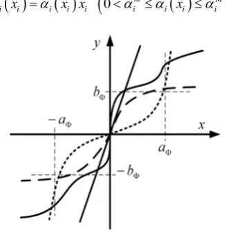
Definition 1: FΦ
(
aΦ,bΦ,x)
with aΦ >0, bΦ>0, and x∈R denotes the set of all continuous differential increasing function [12], Φ( )
x , such that( )
0 0 Φ = ,( )
x bΦ, x R x: aΦΦ ≥ ∀ ∈ >
( )
dΦ x dx>0, ∀ ∈x R
[image:3.595.230.394.525.694.2]where stands for the absolute value.
Figure 1 depicts the example curves for the functions belonging to the function set FΦ. For instance, for all x∈R, the functions, arcsinh x
( )
, tanh( )
x , ax+bx3(
)
0, 0
a> b> , sinh
( )
x , ax and so on, all belong to function set FΦ.The output feedback nonlinear general integral controller [11] and observer [12] are given as,
( )
( )
( )
(
)
( )
( )
( ) ( )
(
( )
( )
)
1
1 1 2 2
1
1 1 2 2
ˆ ˆ ˆ ˆ
ˆ ˆ ˆ
n n
n n
u u x u x u x x
v x v x v x
σ
µ α σ φ ϕ σ
σ µ θ σ −
−
= − + + + + − −
= + + +
(7)
( )
(
)
(
)
(
)
(
)
(
)
(
)
( )
(
)
(
( )
( )
( )
)
(
) ( )
(
( )
)
1
1 1
1
1 2 1 1 1
2
2 3 2 1 1
1 1
1 1 1 1 1 2 2
ˆ d ˆ dˆ ˆ ˆ ˆ ˆ
ˆ ˆ ˆ
ˆ
ˆ ˆ ˆ, ˆ ˆ ˆ ˆ ˆ, ˆ ˆ ˆ ˆ ˆ ˆ ˆ
,
n n
n n n n n
x x
x x h x x
x x h x x
x f x w h x x h g x w u x u x u x
g x w x
σ
σ σ σ
ε ε
ε ε σ µ α σ
φ ϕ σ
−
−
−
− − − −
+
= Φ −
= + −
= + −
= + − + Φ − + + + +
− +
(8)
where xˆ∈Rn
is the estimated state; wˆ∈Rl
is the prescient constant parameters and disturbances; µ, ε, ασ
and hj
(
j=1, 2,,n+1)
are all positive constants;( )
ˆ( )
ˆ ˆ 0(
m( )
ˆ M)
i i i i i i i i i
u x =α x x <α ≤α x ≤α ,
( )
ˆ( )
ˆ ˆ 0(
m( )
ˆ M)
i i i i i i i i i
v x =β x x <β ≤β x ≤β ,
( )
ˆi xi
α and βi
( )
xˆi are the slopes of the line segment connecting xˆi to the origin(
i=1, 2,,n)
;φ( )
xˆ( )
(
φ 0 =0)
is used to attenuate the uncertain nonlinear action of f x w(
,)
; θ σ( )
(
0<θm<θ σ( )
<θM)
is applied to reorganize the integrator output; ϕ σ( )
(
ϕ( )
0 =0)
is utilized to improve the integral control per- formance(
0 m d( )
d M)
σ σ σ
α α ϕ σ σ α
< < + ≤ ; f x wˆ ˆ ˆ
(
,)
and g x wˆ ˆ ˆ(
,)
are the normal models of f x w(
,)
and(
,)
g x w , respectively. Φ
( )
belongs to the function set FΦ.Assumptions 3: By the definition of controller (7), it is convenient to suppose that the following inequalities,
(
,)
(
0,) (
,) ( )
xff x w −f w −g x w φ x ≤lφ x (9)
( ) ( )
0 l 0σ ϕ
ϕ σ −ϕ σ ≤ σ σ− (10)
hold for all x∈Dx, w∈Dw and σ , σ0∈R, where
x f
l φ and lϕσ are all positive constants.
By the definitions of u xi
( )
ˆi , v xi( )
ˆi and θ σ( )
, and letting ei = −xi xˆi(
i=1, 2,,n)
, the controller (7) can be written as,(
) ( ) ( )
(
)
1
1 1 2 2 1
1 1 2 2
ˆ ˆ ˆ ˆ
ˆ ˆ ˆ
n n
n n
u x x x x
x x x
σ
µ α α α α σ φ ϕ σ
σ µ β β β
− − = − + + + + − − = + + +
(11)
and the whole closed-loop system can be written as,
(
) (
) ( ) (
) ( )
(
)(
)
(
)(
)
(
)
(
)
1 2 2 3 11 1 2 2 1
1 1 2 2
1 1
1 1 2 2 1 1 2 2
ˆ
, , , ,
,
n n n
n n
n n n n
x x
x x
x f x w g x w x g x w g x w x x x
g x w e e e
x x x e e e
σ
φ ϕ σ µ α α α α σ
µ α α α
σ µ β β β µ β β β
− − − − = = = − − − + + + + + + + + = + + + − + + + (12)
( )
( )
(
)
(
)
(
( ) ( )
)
1 11 2 1 1
2
2 3 2 1
1 1
1 1 1 1 2 2
1
1 1 2 2
ˆ
ˆ
ˆ
n n
n f n n g n n
g n n g
e
e e h e
e e h e
e h e h x x x
e e e x
σ
σ ε ε
ε ε σ µ α α α α σ
µ α α α φ ϕ σ
− − − − − − + − Φ = = − = −
= ∆ − − Φ − ∆ + + + +
+ ∆ + + + − ∆ + (13) where
(
,)
ˆ ˆ ˆ(
,)
f f x w f x w∆ = − , ∆ =g g x w
(
,) (
−g x wˆ ˆ ˆ,)
,and θ σ
( )
is integrated into βi(
i=1, 2,,n)
.By the equation (2) and inequality (4), and choosing µ−1 and 1 1
n n
h ε− −
+ to be large enough, and then setting
0
x = =e and x= =e 0 of the systems (12) and (13), we obtain
(
) (
1)
1( )
0 0
0, 0,
f w g− w =µ α σ− σ +ϕ σ (14)
( )
(
1)
1( )
0 0 0 0 1 ˆ0
n
f g µ α σσ ϕ σ ε hn σ
− − −
+
∆ − ∆ + = Φ (15)
where
(
)
(
)
0 0, ˆ 0,ˆ
f f w f w
Thus, we ensure that σ0 and σˆ0 are the unique solutions of the systems (12) and (13), respectively.
Defining T T
0
z=x σ σ− , e0 = Φ
( )
σˆ − Φ( )
σˆ0 andn i
i ei
η =ε− +
(
)
0,1, 2, ,
i= n , and substituting (14)
and (15) into (12) and (13), respectively, the whole closed-loop system can be rewritten as,
( )
( )
,,
z z
z A z F z e
Aη Fη z e
εη η ε
= +
= +
(16)
where
1 1 1 1
1 2
1 1 1
1 2
0 1 0 0
0 0 0 0
0 0 1 0
0
z
n
n
A
σ
µ α µ α µ α µ α
µ β µ β µ β
− − − −
− − −
=
− − − −
,
1 2
1 1
0 1 0 0 0 0
0 1 0 0 0
0 0 0
0 0 0 1 0
0 0 0 0 1
0 0 0 0
n
n n
h h A
h
h h
η
− +
−
−
=
−
− −
,
( )
1 1 T1 2 3
, 0 0
z
F z e = δ +µ δ− −µ δ− ,
( )
1 T1 2
, 0 0 0
Fη z e = ∆ +µ−∆ ,
(
) (
) ( )
(
) (
) ( ) ( )
(
)
(
) (
) (
) (
1)
1 f x w, g x w, xˆ f 0,w g x w, 0 g x w, g 0,w f 0,w g 0,w
δ = − φ − − ϕ σ −ϕ σ − − −
,
(
)
(
)
2 g x w, 1 1e 2 2e n ne
δ = α +α + + α ,
3 1 1e 2 2e n ne δ =β +β + + β ,
( )
(
( ) ( )
)
(
)
(
) (
1)
1 f f0 gφ xˆ g ϕ σ ϕ σ0 g g0 f 0,w g 0,w−
∆ = ∆ − ∆ − ∆ − ∆ − − ∆ − ∆ ,
(
)
(
(
)
)
2 g α1 1e α2 2e αn ne g α1 1x α2x2 αnxn α σ σσ 0
∆ = ∆ + + + − ∆ + + + + − ,
and g x w
(
,)
is integrated into αi and ασ.By Assumptions 2 and 3, the uncertain terms δ1, δ2, δ3, ∆1 and ∆2 satisfy the linear growth bound,
( )
1 1
1
z
z η
δ δ
δ ≤γ +γ ε η (17)
( )
2 2η δ
δ ≤γ ε η (18)
( )
3 3η δ
δ ≤γ ε η (19)
( )
1 1
1
z
z η
γ∆ γ∆ ε η
∆ ≤ + (20)
( )
2 2
2
z
z η
γ∆ γ∆ ε η
∆ ≤ + (21)
where γδz1, 1
( )
η δ
γ ε , γδη2
( )
ε , 3( )
η δ
γ ε , γ∆z1, 1
( )
η
γ∆ ε , 2
z
γ∆ and 2
( )
η
3. Propositions on Equal Ratio Gain Technique
Equal ratio gain technique is firstly proposed by [10] and is extended to the canonical interval system matrix in
[11]. For analyzing the stability of the closed-loop system (16), it is necessary to review two important proposi-tions on Equal ratio gain technique as follows.
Proposition 1 [10]: as any row controller gains, or controller and its integrator gains of a canonical system matrix tend to infinity with the same ratio, if it is always Hurwitz, and then the samerow solutions of Lyapunov equation all tend to zero.
Proposition 2 [11]: a canonical interval system matrix can be designed to be Hurwitz as any row controller gains, or controller and its integrator gains increase with the same ratio.
Based on two Propositions above, it is not enough to analyze the stability of the closed-loop system (16). So, a new proposition on Equal ratio gain technique is demonstrated in the next two subsections.
3.1. New Proposition
Consider the following controllable canonical interval system matrix A,
1 1 1 1
1 2 1
1 1 1
1 2
0 1 0 0
0 0 0 0
0 0 1 0
0
n n
n
A
µ α µ α µ α µ α
µ β µ β µ β
− − − −
+
− − −
=
− − − −
where
(
)
0 m M 1, 2, , 1
i i i i n
α α α
< ≤ ≤ = + ,
(
)
0<βmj ≤βj ≤βMj j=1, 2,,n , and µ is a positive constant.
By Proposition 2, the interval system matrix A can be designed to be Hurwitz for all 0<αim ≤α αi ≤ iM,
0 m M
j j j
β β β
< ≤ ≤ and 0< <µ µ∗. Thus, for any given positive define symmetric matrix Q there exists a unique positive define symmetric matrix P that satisfies Lyapunov equation PA+A PT = −Q, and the solution of Lyapunov equation can be obtained by skew symmetric matrix approach [13], that is,
(
)
10.5
P= S−Q A−
where
T
S=PA−A P and A ST +SA=A Q QAT − .
The inversion of the matrix A with µ=1 is,
( )
(
)
1 1 1
1 1
1 1 1 1
0
1 0 0 0 0 0 1 0 0 0 0 0 0
0 0 1 0 0
n n
A
β
α α α β
−
−
− −
+ +
∗ ∗ ∗
=
∗ ∗ ∗ − −
(22)
where the elements ∗ are omitted since it is useless to achieve our object. The interesting reader can evaluate them by AA−1=I
.
Q=I and n=2 of the system matrix A. Thus, taking µ=1, obtain, 12 13
12 23
13 23 1
1 1
s s
S Q s s
s s
−
− = − −
− − −
( )
( )
(
)
1 1 1
1 1
3 1 3 1
0
1 0 0
A
β
α α α β
−
−
− −
∗
=
∗ − −
where
(
)
(
)
1 1 3 2 1 1 1 1 2 2 2 1 2 12
2 3 2 1 3 1
s α α α β α β β α β β α β β
α α β α α β
+ + + + −
=
+ −
(
)
1 2 2 3 2 1 2 2 1 2 3 3 3 1
13
2 3 2 1 3 1
s α α β α β β α α β α α α α β
α α β α α β
− − − −
=
+ −
(
)
(
)
3 3 3 2 1 3 2 2 2 1 23
2 3 2 1 3 1
s α α α β α α β β α β
α α β α α β
+ + + +
= −
+ −
and then we have,
1
13 13
1 3 1
1 2 2
p s α
β α β
= − −
23 3
1 2
p α
=
13 1
33
1 3 1
2 2
s
p α
β α β
= − +
Now, α3, α2, α1, β2 and β1 are multiplied by
1 µ−
, then we obtain,
(
)
(
)
2
1 1 3 2 1 1 1 1 2 2 2 1 2 12
2 3 2 1 3 1
sµ α µ α µ α β α β β µ α β β α β β α α β µα µα β
+ + + + −
=
+ −
(
)
1 2 2 3 2 1 2 2 1 2 3 3 3 1
13
2 3 2 1 3 1
sµ α α β α β β α α β µα α α α β α α β µα µα β
− − − −
=
+ −
(
)
2
3 3 3 2 1 3 3 2 2 2 1 23
2 3 2 1 3 1 sµ µ α α α β µα α α β β µα β
α α β µα µα β
+ + + +
= −
+ −
1
13 13
1 3 1
1
2 2
p µ sµ α µ
β α β
= − −
23 3
1 2
p µ
α
=
13 1
33
1 3 1
2 2
s p
µ α
µ µ
β α β
= − +
It is obvious that s12
µ
, s23
µ
and s13
µ
3 3 0
P = Pµ µ→ as µ→0
where P3 P3
[
p31 p32 p33]
µµ
= = .
From the statements above, it is easy to see that for n=2 of the system matrix A, P3 can be formulated as the linear form on µ and tends to zero as µ→0. Moreover, the solution of the matrix S is more and more complex as the order of the system matrix A increases. Thus, by the inversion of system matrix A−1
(22),
1
n
P+ can be formulated as the linear form on µ for the n+1-order system matrix A, and with the help of
computer, it can be verified that the solution of Pn 1
µ
+ still tends to the constant as µ→0. Therefore, for the
1
n+ -order system matrix A, we can conclude that Pn+1 →0 as µ→0. As a result, the following theorem can be established.
Theorem 1: If the interval system matrix A is Hurwitz for all 0<αim ≤α αi ≤ iM, 0
m M
j j j
β β β
< ≤ ≤ and 0< <µ µ∗, and then we have,
1 1 0
n n
P+ = Pµ+ µ→ as µ→0.
where
1 1 1,1 1,2 1, 1
n n n n n n
P+ =Pµ+µ= p+ p+ p+ + ,
1 1 1 1 1 1
1 0.5 1 1 1, 1 1 1 12 2, 1 1 1 1, 1 1, 1 1 1 1 1 1, 1 1 1
n n n n n n n n n n n n
Pµ+ = − β− +sµ+α α−+ sµ +sµ +α α−+ sµ− +sµ− +α α−+ β α−+ sµ+ +α α−+ .
Discussion 1: From the statements above, the solution of the matrix S is more and more complex as the order of the system matrix A increases. So, although Theorem 1 is demonstrated by taking Q=I and the single va-riable system matrix A, it is very easy to extend Theorem 1 to any given positive define symmetric matrix Q and the multiple variable system matrix A with the help of computer since there is not any difficulty to obtain the solution of the matrix S in theory, that is, Lyapunov equation applies to not only the single system matrix but also the multiple system matrix. Thus, there is the following proposition.
Proposition 3: as any row integrator and its controller gains of a canonical interval system matrix tend to in-finity with the same ratio, if it is always Hurwitz, and then the samerow solutions of Lyapunov equation all tend to zero.
3.2. Example
For testifying the justification of Theorem 1 and Proposition 3, we consider a 6-order two variable system ma-trix A as follows,
1 2 3 4
1 2 3 4
1 2 3 4 5
1 2 3 4 5
0 0 0 0 1 0
0 0 0 0 0 1
0 0
0 0
0 0
x x x x
y y y y
x x x x x
y y y y y
A ββ ββ ββ ββ
α α α α α
α α α α α
=
− − − − −
− − − − −
The inversion of the system matrix A is,
13 14 23 24 33 34 35 1
43 44 46
0 0
0 0
0 0
1 0 0 0 0 0
0 1 0 0 0 0
a a
a a
a a a
A
a a a
−
∗ ∗
∗ ∗
∗ ∗
= ∗ ∗
(
)
(
)
(
)
2 1 1 2 2 1
13 23 33
2 1 1 2 2 1 1 2 3 2 1 1 2
1 2 2 1 2 1
43 14 24
2 1 1 2 2 1 1 2 3 2 1 1 2
1 2 2 1 34
3 2 1 1 2
, ,
, ,
,
y y x y x y
x y x y x y x y x x y x y
y y y y x x
y x y x y x y x
y x y x y
x x x x
x y x y x
a a a
a a a
a
β β α β α β
β β β β β β β β α β β β β
α β α β β β
β β β β β β β β
α β β β β
α β α β
α β β β β
−
= − = =
− − −
−
= = − =
− −
− − =
−
(
)
1 2 2 1
44 35 46
3 3
3 2 1 1 2
1 1
, , .
y x y x
x y
y y x y x
a α β α β a a
α α
α β β β β
−
= = − = −
−
By the equation A ST +SA=A Q QAT − , it is very easy to obtain the fifteen linear equations with fifteen ele-ments of the matrix S. So, it is omitted.
Thus, taking
0 0 0 0 1 0
0 0 0 0 0 1
8 2 0 0 3 1
2 7 0 0 1 5
8 2 8 0 3 1
2 8 0 8 1 3
A
=
− − − − −
− − − − −
3.0 1.0 0.8 0.6 0.5 0.3 1.0 5.0 1.3 1.0 0.8 0.2 0.8 1.3 6 0.8 0.4 1.0 0.6 1.0 0.8 2.0 1.3 0.5 0.5 0.8 0.4 1.3 3.0 0.8 0.3 0.2 1.0 0.5 0.8 6.0 Q
−
−
=
.
Now, by Routh’s stability criterion and with the help of computer, we have: 1) if αix
(
i=1, 2,, 5)
andx j
β
(
j=1, 2,, 4)
of the system matrix A are multiplied by µ−1, then it is still Hurwitz for all 0< ≤µ µ∗=1.45, and the numerical solutions of P3 are shown in Table 1; 2) ify i
α and βjy of the system matrix A are multiplied by µ−1, then it is still Hurwitz for all 0< ≤µ µ∗ =2.90, and the numerical solutions of P4 are shown in Table 2.
From the example above, it is obvious that: 1) as shown in Table 1, Table 2, the absolute values of p3i and
4i
[image:9.595.237.389.237.424.2] [image:9.595.87.542.568.718.2]p
(
i=1, 2,, 6)
are all decrease as µ reduces; 2) although the result above is obtained by a constant sys-tem matrix, it is easy to be extended to the interval syssys-tem matrix. This not only verifies the justification of Theorem 1 and Proposition 3 but also shows that for the high order and multiple variable system matrix, it is convenient and practical with the help of computer.Table 1.Numerical Solutions of P3 for all
x i
α and βjx multiplied by
1
µ− .
1.0
µ= µ=0.1 µ=0.01
31
p 21.38 4.54e-1 4.27e-2
32
p −5.90 1.66e-1 1.81e-2
33
p 25.78 5.65e-1 5.32e-2
34
p −10.86 −2.32e-1 −2.24e-2
35
p 0.75 7.50e-2 7.5e-3
36
Table 2. Numerical Solutions of P4 for all
y i
α and βjy multiplied by
1
µ− .
1.0
µ= µ=0.1 µ=0.01
41
p −6.73 6.23e-2 7.70e-3
42
p 6.27 3.09e-1 2.97e-2
43
p −10.86 −3.13e-1 −3.10e-2
44
p 9.45 4.10e-1 3.93e-2
45
p 0.94 1.55e-1 1.60e-2
46
p 0.25 2.50e-2 2.50e-3
4. Stability Analysis
The asymptotic stability of the closed-loop system (16) can be achieved by Equal ratio gain technique and Sin-gular perturbation technique as follows:
By Proposition 2 [11], the interval system matrix Az can be designed to be Hurwitz for all
0 m M
i i i
α α α
< ≤ ≤ , 0<βmj ≤βj ≤βjM, ασ and 0< <µ µ∗,
and by choosing hj
(
j=1, 2,,n+1)
, the matrix Aη can be designed to be Hurwitz, too. Thus, by linearsystem theory, two quadratic Lyapunov functions,
( )
Tz z
V z =z P z (23)
( )
TVη η =η Pηη (24)
can be obtained. Where Pz and Pη are the solutions of Lyapunov equations,
T
z z z z z
P A +A P = −Q and P A A PT Q
η η+ η η = − η
with any given positive define symmetric matrices Qz and Qη, respectively.
Using V z
( ) (
,η = −1 d V) ( )
z z +dVη( )
η [1] as Lyapunov function candidate, and then its time derivativealong the trajectories of the closed-loop system (16) is,
( ) (
) ( )
( )
(
)
T(
T)
1 T(
T)
(
)
( ) ( )
( ) ( )
, 1
1 1 , , ,
z
z
z z z z z
V z d V z dV
V V z
d z A P P A z d A P P A d F z e d F z e
z
η
η
η η η η η
η η
η
ε η η
η −
= − +
∂ ∂
= − + + + + − +
∂ ∂
(25)
Substituting F z ez
( )
, and Fη( )
z e, into (25), obtain,( ) (
)
(
)
(
)
(
)
(
)
(
)
(
)
(
)
(
)
(
) (
)
T T 1 T T T 1
1 2
T
1 1 T 1 T
1 2 1 3 3 1
T
T 1 1
1 1 2 1 2 1
, 1 1
1 1 1
,
z z z z zn
zn zn zn
n n
V z d z A P P A z d A P P A d z P
d P z d z P d P z
d P d P
η η η η
η η
η ε η η δ µ δ
δ µ δ µ δ µ δ
η µ µ η
− −
− − −
+ +
− −
+ +
= − + + + + − +
+ − + − − − −
+ ∆ + ∆ + ∆ + ∆
(26)
where
1 2 , 1
zn n n n n
P = p p p + ,
1 1,1 1,2 1, 1
zn n n n n
P + = p+ p+ p+ + ,
1 1,1 1,2 1, 1
n n n n n
Now, by Propositions 1 and 3, we have,
0
zn zn
P = Pµ µ→ as µ→0,
1 1 0
zn zn
P + = Pµ+ µ→ as µ→0.
Substituting them and (17) - (21) into (26), obtain,
( )
(
)
(
( )
)
(
)
(
( )
( )
)
(
) ( )
(
)
(
)
( )
(
( )
( )
)
1
1 2 3 1 2
1 2 2 1 1 1 2 1 1 T
, 1 2
2 1 1 1
2 ,
z
m z zn
z z
zn zn n
m n
V z d Q P z
d P d P d P z
Q d P
µ δ
η η µ η µ
δ δ δ η
η η
η η
η λ µγ
µγ ε γ ε γ ε γ µ γ η
λ γ ε µ γ ε η
ε ζ ζ − + ∆ ∆ + − ∆ ∆ + ≤ − − − + − + + − + + − − +
= − Λ
(27)
where
T
z
ζ = η ,
( )
2 1z z
z m Qz Pzn
µ δ
ρ =λ − µγ ,
( )
( )
(
1 2)
3( )
1z Pzn Pzn
η η η µ η µ
δ δ δ
ρ = µγ ε +γ ε +γ ε + ,
(
1 2)
1
1
z z z
n P
η η
ρ γ µ γ−
∆ ∆ + = + ,
( )
m Q η η ηρ =λ ,
( )
( )
(
1 2)
1
1
2 η η Pn
η η
γ γ ε µ γ− ε
∆ ∆ + = + ,
(
)
(
)
(
)
1 1 1 1 z z z z z zd d d
d d d
η η
η η
η η η
ρ ρ ρ
ρ ρ ρ γ
ε
− − − −
Λ =
− − − −
.
The right-hand side of the inequality (27) is a quadratic form, which is negative define when,
(
)
(
1)
(
(
)
)
21 d d zz 1 d z d z
η η
η η η
ρ ε ρ− γ ρ ρ
− − > − + (28)
This is equivalent to,
(
)
(
)
(
(
)
)
21 1 1 z z d z z z z d d
d d d d
η η η η η ρ ρ ε ε
ρ γ ρ ρ
− < =
− + − + (29)
By the dependence of εd on d, it is obvious that the maximum of εd occurs at
(
)
* z
z z
d =ρη ρη +ρη [1]
and is given by,
4
z z
d z z
z z η η η η η ρ ρ ε ε
ρ γ ρ ρ
∗ < =
+ (30)
Although Pzn
µ
and Pzn1
µ
+ are dependent on xˆ, they are fixed for any given moment t and all tend to
the constants as µ→0, and then there exists µ∗∗
( )
t such that ρzz >0 holds for all 0 µ( )
t µ( )
t ∗∗< < .
Thus, by choosing a moderate µ
( )
t and solving the Equation (30), ε µ∗(
( )
t)
can be obtained, and then 0[
0,)
t∈ ∞ , then we conclude that V z
( )
,η ≤0 holds uniformly in t.Using the fact that Lyapunov function V z
( )
,η is a positive define function and its time derivative is a nega-tive define function if Λ >0 holds for all t∈[
0,∞)
, we conclude that the closed-loop system (16) is stable. In fact, V z( )
,η =0 means x=0, e=0, σ σ= 0 and σ σˆ= ˆ0. By invoking LaSalle’s invariance principle, it iseasy to know that the closed-loop system (16) is uniformly exponentially stable. As a result, we have the fol-lowing theorem.
Theorem 2: Under Assumptions 1, 2 and 3, if the matrix Aη is Hurwitz and the interval system matrix Az is Hurwitz for all 0< <µ µ∗, 0<αim ≤α αi ≤ iM, 0
m M
j j j
β β β
< ≤ ≤ and ασ , and then the equilibrium point
0
x= , e=0, σ σ= 0 and σ σˆ= ˆ0 of the closed-loop system (16) is uniformly exponentially stable for all
( )
( )
0<µ t <µ∗∗ t and 0<ε
( )
t <ε µ∗(
( )
t)
. Moreover, if all assumptions hold globally, and then it is globally uniformly exponentially stable.By the demonstration above, there exist µ∗∗
( )
t and ε µ∗(
( )
t)
such that ρzz >0 and Λ >0 hold for all[
0,)
t∈ ∞ . So, it is practical and feasible to find a real method to evaluate the instantaneous values µ∗∗
( )
t and( )
(
t)
ε µ∗
, that is, as follows:
Step 1: by the inequality m
( )
Qz 2 z1 Pzn( )
tµ δ
λ > µγ , the impermissible minimum of Pzn
( )
t m is,( )
0.5( )
z1zn m m z
P t = λ Q γδ
Step 2: by the definitions of αi
( )
xˆi and βi( )
xˆi , the instantaneous values αi( )
t and βi( )
t can be givenas,
( )
(
( )
( )
)
( )
( )
(
( )
( )
)
( )( )
ˆ 0 ˆ ˆ, if 0;
ˆ
ˆ d
ˆ if 0. ˆ d i i i i i i i i i i i x t
u x t
t x t
x t
u x t
t x t
x t α α = = ≠ = =
( )
(
( )
( )
)
( )
( )
(
( )
( )
)
( )( )
ˆ 0 ˆ ˆ, if 0;
ˆ
ˆ d
ˆ if 0. ˆ d i i i i i i i i i i i x t
v x t
t x t
x t
v x t
t x t
x t β β = = ≠ = =
Step 3: by the values Pzn
( )
t m, αi( )
t , βi( )
t and the condition 0 µ µ∗
< < , and using the iterative me-thod to solve Lyapunov equation,
( ) ( )
T( ) ( )
z z z z z
P t A t +A t P t = −Q
( )
t µ∗∗can be obtained. Thus, by choosing a moderate µ
( )
t and solving Lyapunov equation above again,( )
zn
Pµ t and Pzn 1
( )
tµ
+ can be evaluated.
Step 4: by the values αi
( )
t , βi( )
t and definitions ofn i
i ei
η =ε− +
, δ1 δ2, δ3, ∆1 and ∆2, 1
z
δ
γ , γ∆z1,
2
z
γ∆ , 1
( )
η δ
γ ε , γηδ2
( )
ε , γδη3( )
ε , γη∆1( )
ε and 2( )
η
γ∆ ε can be obtained for given ε. Pη +n 1 can be eva-luated by solving Lyapunov equation P A A PT Q
η η+ η η = − η.
Step 5: by the values Pzn
( )
tµ
, Pzn1
( )
tµ
+ , Pη +n 1 , 1
z
δ
γ , γ∆z1, 2
z
γ∆ , 1
( )
η δ
γ ε , γηδ2
( )
ε , 3( )
η δ
γ ε , γη∆1
( )
ε and( )
2η
γ∆ ε , and using the iterative method to solve the inequality (30), ε µ∗
(
( )
t)
can be obtained.5. Example and Simulation
Consider the pendulum system [1] described by,
( )
sin
a b cT
θ= − θ − θ+
where a b c, , >0, θ is the angle subtended by the rod and the vertical axis, and T is the torque applied to the pendulum. View T as the control input and suppose we want to regulate θ to r. Now, taking x1= −θ r,
2
x =θ, the pendulum system can be written as,
(
)
1 22 sin 1 2
x x
x a x r bx cu
=
= − + − +
and then it can be verified that u0 =asin
( )
r c is the steady-state control that is needed to maintain equilibrium at the origin.The nonlinear general integral controller and the integral observer can be given as,
( )
( )
(
)
( )
( )
( )
( )
(
)
1
1 1 2 2 1
1
1 1 2 2
ˆ ˆ ˆ ˆ ˆ
3 3sinh 3 tanh 4 0.3tanh 4sin 3 ˆ ˆ ˆ ˆ
3 sinh 2tanh
u x x x x x
x x x x
µ σ σ
σ µ −
−
= − + + + + − +
= + + +
( )(
)
(
)
(
)
(
)
( )
1
1 1
1
1 2 1 1
2 3
2 1 1 1
ˆ cosh ˆ ˆ ˆ ˆ 5 ˆ
ˆ 10 sin ˆ 7.5 20 ˆ 5sinh ˆ
x x
x x x x
x x r u x x
σ σ
ε
ε ε σ
−
−
− −
= −
= + −
= − + − + − +
Thus, it is easy to obtain 6≤α1<14.1, 3≤α2≤4, ασ =4, 4≤β1<6.68 and 1<β2≤3, and then the
closed-loop system can be written as,
( )
( )
,,
z z
z A z F z e
Aη Fη z e
εη η ε
= +
= +
where
[
]
T1 2 0
z= x x σ σ− ,
( )
( )
0 sinh ˆ sinh ˆ0e = σ − σ ,
(
)
ˆ 1, 2
i i i
e = −x x i= ,
(
)
2 j 0,1, 2
j ej j
η =ε− + = ,
(
)
1 1 1 1
1 2
1 1
1 2
0 1 0
0
z
A µ αc µ c α µc b µ αc σ
µ β µ β
− − − −
− −
= − − + −
,
0 1 0
0 5 1
5 20 0 Aη
= −
− −
,
( )
1 1 T1 2 3
, 0
z
F z e = δ +µ δ− −µ δ− ,
( )
1 T1 2
, 0 0
(
)
( )
( )
(
( )
( )
)
1 asin x1 r asin r 4 sinc xˆ1 3 0.3c tanh tanh 0δ = − + + + − σ − σ ,
(
)
2 c 1 1e 2 2e
δ = α +α ,
3 1 1e 2 2e
δ =β +β ,
(
)
( )
(
)
(
(
)
( )
)
(
)
(
( )
( )
( )
)
1 a sin x1 r sin r aˆ sin xˆ1 r sin r bx2 c cˆ 4sin xˆ1 3 0.3tanh σ 0.3tanh σ0
∆ = − + − + + − − + − − + ,
(
)(
) (
)
(
(
)
)
2 c cˆ α1 1e α2 2e c cˆ α1 1x α2x2 α σ σσ 0
∆ = − + − − + + − .
The normal parameters are a= =c 10 and b=2, and in the perturbed case, b and c are reduced to 1 and 5, respectively, corresponding to double the mass. Thus, with 1 6
m
α = , 2 3
m
α = , ασ =4, 1 6.68
M
β = ,
2 1
m
β = , c=5 and b=1, the following inequality,
(
)
2
2 2 1 2 1 2 1 0
m m m m m m M
cα α βσ +µ αb +µ α αc +bα βσ −α βσ >
holds for all 0< < ∞µ , and then the matrix Az is Hurwitz for all 6≤α1<14.1, 3≤α2 ≤4, ασ =4, 1
4≤β <6.68, 1<β2≤3 and 0< < ∞µ , and Aη is Hurwitz, too.
Now, solving Lyapunov equation, T
P Aη η+A Pη η = −I, obtain Pη +n 1 ≤0.57, and using aˆ=10, cˆ=7.5, 10
c= , b=2, obtain,
1 4.5 z 13.4
δ ≤ + ε η ,
( )
( )
2 2 2
2 10 1 t 2 t
δ ≤ ε α +α η ,
( )
( )
2 2 2
3 1 t 2 t
δ ≤ ε β +β η ,
1 4.9 z 13.4ε η
∆ ≤ + ,
( )
( )
( )
( )
2 2 2 2 2 2
2 2.5 ε α1 t α2 t η 2.5 α1 t α2 t ασ z
∆ ≤ + + + + ,
and then, we have,
1 4.5
z
δ
γ = , 2
( )
2 2( )
2( )
1 2
10 t t
η δ
γ ε = ε α +α ,
( )
1 13.4η δ
γ ε = ε, 3
( )
2 12( )
t 22( )
tη δ
γ ε = ε β +β ,
( )
1 13.4η
γ∆ ε = ε, 2
( )
( )
( )
2 2 2
1 2
2.5 t t
η
γ∆ ε = ε α +α ,
1 4.9
z
γ∆ = , 2
( )
( )
2 2 2
1 2
2.5
z
t t σ
γ∆ = α +α +α .
Thus, using α1
( )
t , α2( )
t , β1( )
t , β2( )
t , ασ =4, c=5, b=1 and µ=1 to solve the equations, Tz z z z
P A +A P = −I and z
(
z 4 z)
z z z
η η
η η η
ε ρ ρ= ρ γ + ρ ρ , ε∗
( )
t can be obtained.Now, taking µ=1 and ε
( )
t =ε∗( )
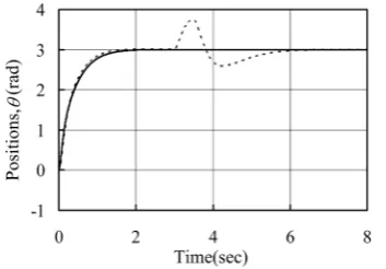
t , the simulation is implemented under the normal and perturbed cases, respectively.Normal case: the initial states are x1=xˆ1= −3.0 and x2=xˆ2=0; the system parameters are a= =c 10 and b=2.
Perturbed case: the initial states are x1=xˆ1= −3.0, x2= −1.5 and xˆ2=0; the system parameters are 10
a= , b=1 and c=5, corresponding to doubling of the mass. Moreover, we consider an additive im-pulse-like disturbance d t
( )
of magnitude 60 acting on the system input between 3 s and 3.5 s.Figure 2 and Figure 3 showed the simulation results under the normal (solid line) and perturbed (dashed line) cases. The following observations can be made: 1) as µ=1, there exists ε∗
( )
t such that z 0z
Figure 2. The values of 100ε under normal (solid line) and perturbed case (dashed line).
Figure 3. System output under normal (solid line) and per-turbed case (dashed line).
hold for all α1
( )
t , α2( )
t , β1( )
t and β2( )
t . This shows that the closed-loop system is uniformly asymptotic stable. 2) the optimum responses are almost identical before the additive impulse-like disturbance appears. This means that by Equal ratio gain technique and Singular perturbation technique, we can tune an output feedback nonlinear general integral controller with good robustness and high control performance. All these demonstrate that output feedback nonlinear general integral control has the striking robustness, that is, so long as the bounded conditions are satisfied, the asymptotically stable control can be achieved, but also the organic combination of Equal ratio gain technique and Singular perturbation technique constitutes a powerful and practical tool to solve the output feedback control design problem of dynamics with the nonlinear and uncertain actions.6. Conclusions
This paper proposes an output feedback nonlinear general integral controller for a class of uncertain nonlinear system. The main contributions are that: 1) as any row integrator and its controller gains of a canonical interval system matrix tend to infinity with the same ratio, if it is always Hurwitz, and then the samerow solutions of Lyapunov equation all tend to zero; 2) theorem to ensure regionally as well as semi-globally exponential stabili-ty is established in terms of some bounded information; 3) a real time method to evaluate the ratio coefficients of controller and observer are proposed such that their values can be chosen moderately.
Theoretical analysis and simulation results show that not only output feedback nonlinear general integral con-trol has the striking robustness but also the organic combination of Equal ratio gain technique and Singular per-turbation technique constitutes a powerful tool to solve the output feedback control design problem of dynamics with the nonlinear and uncertain actions.
References
[1] Khalil, H.K. (2007) Nonlinear Systems. 3rd Edition, Electronics Industry Publishing, Beijing, pp. 551, 449-453.
[2] Liu, B.S. and Tian, B.L. (2012) General Integral Control Design Based on Linear System Theory. Proceedings of the
[image:15.595.230.400.85.209.2] [image:15.595.227.404.250.373.2][3] Liu, B.S. and Tian, B.L. (2012) General Integral Control Design Based on Sliding Mode Technique. Proceedings of the
3rd International Conference on Mechanic Automation and Control Engineering, Vol.5, 3178-3181.
[4] Liu, B.S., Li, J.H. and Luo, X.Q. (2014) General Integral Control Design via Feedback Linearization. Intelligent Con-trol and Automation, 5, 19-23. http://dx.doi.org/10.4236/ica.2014.51003
[5] Liu, B.S., Luo, X.Q. and Li, J.H. (2014) General Integral Control Design via Singular Perturbation Technique. Interna-tional Journal of Modern Nonlinear Theory and Application, 3, 173-181. http://dx.doi.org/10.4236/ijmnta.2014.34019
[6] Liu, B.S., Luo, X.Q. and Li, J.H. (2013) General Concave Integral Control. Intelligent Control and Automation, 4, 356-361. http://dx.doi.org/10.4236/ica.2013.44042
[7] Liu, B.S., Luo, X.Q. and Li, J.H. (2014) General Convex Integral Control. International Journal of Automation and Computing, 11, 565-570. http://dx.doi.org/10.1007/s11633-014-0813-6
[8] Liu, B.S. (2014) Constructive General Bounded Integral Control. Intelligent Control and Automation, 5, 146-155.
http://dx.doi.org/10.4236/ica.2014.53017
[9] Liu, B.S. (2014) On the Generalization of Integrator and Integral Control Action. International Journal of Modern Nonlinear Theory and Application, 3, 44-52. http://dx.doi.org/10.4236/ijmnta.2014.32007
[10] Liu, B.S. (2015) Equal Ratio Gain Technique and Its Application in Linear General Integral Control. International Journal of Modern Nonlinear Theory and Application, 4, 21-36. http://dx.doi.org/10.4236/ijmnta.2015.41003
[11] Liu, B.S. (2014) Nonlinear General Integral Control Design via Equal Ratio Gain Technique. International Journal of Modern Nonlinear Theory and Application, 3, 256-266.http://dx.doi.org/10.4236/ijmnta.2014.35028
[12] Liu, B.S., Luo, X.Q. and Li, J.H. (2014) Conventional and Added-Order Proportional Nonlinear Integral Observers.
International Journal of Modern Nonlinear Theory and Application, 3, 210-220.
http://dx.doi.org/10.4236/ijmnta.2014.35023