A Hybrid Algorithm for Solving Steiner Tree Problem
Samira Noferesti
Electrical and Computer Engineering Department, University of Sistan and Baluchestan, Iran
Hamed Shah-Hosseini
Electrical and Computer Engineering Department, Shahid BeheshtiUniversity
ABSTRACT
In this paper, a hybrid algorithm based on modified intelligent water drops algorithm and learning automata for solving Steiner tree problem is proposed. Since the Steiner tree problem is NP-hard, the aim of this paper is to design an algorithm to construct high quality Steiner trees in a short time which are suitable for real time multicast routing in networks. The global search and fast convergence ability of the intelligent water drops algorithm make it efficient to the problem. To achieve better results, we used learning automata for adjusting IWD parameters. IWD has several parameters. The appropriate selections of these parameters have large effects on the performance and convergence of the algorithm. Experimental results on the OR-library test cases show that the proposed algorithm outperforms traditional heuristic algorithms and other iteration based algorithms with faster convergence speed.
General Terms
Keywords
Intelligent water drops algorithm; Steiner tree problem; Learning automata; Parameter adaptation
1.
INTRODUCTION
Multicasting is the ability of a communication network which allows a source node to communicate with multiple destination nodes. One way to establish a multicast session is to build a multicast tree connecting the members of the multicast group. This multicast tree is rooted at the source node and spans all destination nodes such that the communication cost becomes minimized. Multicast routing problem has many applications such as audio and video conferencing and multiplayer games. Recently, with the high demand of real time communication services, most researchers have focused on developing algorithms that produce high quality multicast trees with low computational cost. One of the most popular algorithms for building multicast trees in networks is Steiner tree algorithms [1,2]. The Steiner minimum tree (SMT) is the shortest network spanning a set of nodes called terminals with the use of additional points named Steiner points. The determination of a Steiner tree is NP-complete and hard even to approximate In this paper a hybrid algorithm based on intelligent water drops (IWD) algorithm and learning automata is proposed for solving the Steiner tree problem in graphs. The IWD algorithm was first introduced in [3] and has been used for some of well-known NP-hard combinatorial optimization problems such as the travelling salesman problem (TSP) [4],
multiple knapsack problems (MKP), n-queen puzzle, automatic multilevel thresholding [5] and economic load dispatch [6] and reached promising results. We use the modified IWD algorithm called EIWD in which some elitist IWDs perform global soil updating instead of the best-iteration IWD. In order to overcome the problem of premature convergence, when all elitist IWDs produce the same tree the amount of soil on all edges of the graph is set to the initial value and then global soil updating is done for the best resulted tree. Also, to achieve better results learning automata are used for adjusting IWD parameters. Simulation results show that these extensions improve the original IWD algorithm for solving Steiner tree problem.
The rest of the paper is organized as follows. Section 2, formally defines the Steiner tree problem and reviews the previous works to solve it. A brief description of the IWD algorithm and the proposed algorithm for solving Steiner tree problem is given in section 3. Section 4 describes learning automata based approach for adaptation of IWD parameters. Simulation results are presented in Section 5. Finally section 6 concludes the paper.
2.
THE STEINERT TREE PROBLEM
AND RELATED WORKS
Two famous special cases of the Steiner tree problem are the Euclidean Steiner tree and rectilinear Steiner tree. In both problems the task is to find a shortest tree connecting given points in the plane. The only difference in these special cases is the metric used to measure distances. In the Euclidean Steiner tree problem distances are measured by the L2, i.e. the Euclidean metric, while in the rectilinear Steiner tree problem distances are measured by the L1 metric [7,8]. These two special cases of the Steiner tree problem have been studied intensely. However, Steiner tree problems arising in practical applications usually involve cost functions that do not satisfy the L1 or L2 metric. This motivates the study of the Steiner tree Problem in graphs. Since in the Steiner tree in graphs we do not have any restrictions on the length function for the edges in the graph, we can model any Steiner tree problem in any metric by a Steiner tree problem in graphs.
If the resulted tree just contained terminals, the tree is a minimum spanning tree and many well-known polynomial time algorithms such as Prim’s algorithm [9] have been proposed for solving this problem. However in general, the tree may include some auxiliary non-terminal points called Steiner vertices or Steiner points. Steiner points are used to decrease the overall cost of the tree. As an example, consider the graph of figure 1. In this figure, terminals are numbered with 1, 2, 3 and 4. The Steiner minimal tree includes two Steiner points which are highlighted and has a cost of 8.
Fig 1: An example of the Steiner tree in graph
The Steiner tree problem is NP-hard even in Euclidean or rectilinear metrics [10-12]. A lot of works have been done to find exact algorithms as well as heuristic approaches to solve the Steiner tree problem. Exact algorithms usually based on dynamic programming and branch and cut algorithms [7] require significant computational effort and they aren’t appropriate for most practical applications such as multicast routing in networks. Therefore much more previous efforts were heuristic algorithms [7, 13-15] such as the shortest path heuristic (SPH), the distance network heuristic (DNH) and the average distance heuristic (ADH) [16]. Most of the traditional heuristic algorithms either need long computational time or generate low quality solutions.
After introducing evolutionary algorithms, genetic algorithms have been successfully used for building Steiner trees [17-18]. These algorithms reach good results but may encounter the long computational time to obtain the solutions because they have to iterate many generations to converge. In recent years, swarm intelligence approaches such as particle swarm intelligence (PSO) [19-20] and ant colony optimization (ACO) [2,21] have been successfully applied to the Steiner tree problem. In this paper we pursue these approaches and use the modified IWD algorithm with learning automata for parameter adaptation.
3.
THE IWD ALGORITHM
Intelligent Water Drops or IWD is a new swarm intelligence technique based on observation of natural water drops moving in rivers, lakes and seas. Natural water drops which follow in a river often find good paths among lots of possible paths. These near optimal or optimal paths are obtained by cooperation among the water drops and the water drops with the riverbeds.
In IWD algorithm, water drops move from source to destination in discrete time steps. Each IWD has two attributes: soil and velocity and begins its trip with an initial velocity and zero soil. During its trip, each IWD removes some soil from the riverbed and transfers soil from one place to another place. The amount of soil which an IWD is gathered from the bed depends on its velocity. Faster water drops can gather and transfer more soil. In addition, when an IWD encounters several paths, it needs a mechanism to select
among them. Water drops prefer to select the paths which have low soil [4-5]. In the following, we introduce the IWD algorithm to solve the Steiner tree problem in graphs.
3.1
The IWD Algorithm for Solving
Steiner Tree Problem
In the first step, the SMT problem should be represented in a suitable way for IWD algorithm. For this reason, the candidate Steiner points in the original graph are numbered from 1 to m. Where m is the number of non-terminal nodes. Then a new directed graph (V,E) is constructed where the node set V denotes the candidate Steiner points of the original graph and edge set E denotes the directed edges between nodes. Every node ni has exactly two directed links to the next
node ni+1 called above and below links.
Each IWD begins constructing its solution from the first node n1, then travels from node n1 to n2 and continues its trip until it
reaches the last node nm+1. It means that when an IWD is in
node ni, the next node will be ni+1. Selecting the above link by
the IWD in node ni means that the ith non-terminal node will
be in the Steiner tree. In contrast, selecting the below link means the node ni will not be in the final tree. On the other
hand, each IWD is responsible for extracting appropriate set of Steiner points. The IWD algorithm for solving Steiner tree problem is as follows:
1.The static and dynamic parameters of the IWD algorithm are set to appropriate values. We choose the following parameter values. For velocity updating the parameters are av=1, bv=0.01 and cv=1 and for soil updating the parameters
are as=1, bs=0.01 and cs=1. The initial soil on each link is set
to 10000. The initial velocity and soil of each IWD is set to 200 and 0 respectively. The global soil updating parameter 𝜌𝑖𝑤𝑑 is set to 0.9. 𝜌𝑠 is set to 1.9. The local soil updating parameters 𝜌 is chosen as a negative value -0.9. These values are the same values used in [4].
2.The number of water drops is equal to the number of non-terminal nodes. As be mentioned, the role of each IWD is to construct a solution by selecting some of candidate Steiner points. Thus, each IWD has a list of selected nodes S which is empty at first.
3.At the start of each iteration, all IWDs are placed on the first node n1.
4.The IWD in node i chooses the link l to reach the next node i+1 according to the following probability:
𝑃𝑖,𝑙𝐼𝑊𝐷 =
𝑓 𝑠𝑜𝑖𝑙𝑖,𝑙
𝑓 𝑠𝑜𝑖𝑙𝑖,𝑎𝑏𝑜𝑣𝑒 +𝑓 𝑠𝑜𝑖𝑙𝑖,𝑏𝑒𝑙𝑜𝑤 (1)
f(
𝑠𝑜𝑖𝑙
𝑖,𝑙) = 𝜀 1𝑠+𝑔(𝑠𝑜𝑖𝑙𝑖,𝑙)
(2)
𝑔 𝑠𝑜𝑖𝑙𝑖,𝑙 =
𝑠𝑜𝑖𝑙𝑖,𝑙 𝑖𝑓 𝑚𝑖𝑛𝑗 ∈{𝑎𝑏𝑜𝑣𝑒 ,𝑏𝑒𝑙𝑜𝑤 }𝑠𝑜𝑖𝑙𝑖,𝑗≥ 0
𝑠𝑜𝑖𝑙𝑖,𝑙− 𝑚𝑖𝑛𝑗 ∈{𝑎𝑏𝑜𝑣𝑒 ,𝑏𝑒𝑙𝑜𝑤 }𝑠𝑜𝑖𝑙𝑖,𝑗 𝑜𝑡𝑒𝑟𝑤𝑖𝑠𝑒 (3)
Where 𝑃𝑖,𝑙𝐼𝑊𝐷 is the probability of selecting link l to move to the next node and s is a small positive number which
prevents division by zero in function f(.). 𝑠𝑜𝑖𝑙𝑖,𝑙represents the amount of soil on the output link l of node i. If an IWD selects the link above, node i is added to its set S.
5.Whenever an IWD travels from node i to the next node through link l, its velocity is updated as follows:
𝑣𝑒𝑙𝐼𝑊𝐷 𝑡 + 1 = 𝑣𝑒𝑙 𝑡 + 𝑎𝑣
Where 𝑣𝑒𝑙𝐼𝑊𝐷(𝑡 + 1)is the updated velocity of the IWD. is set to 3 by using trial and error procedure. av,bv and cv are
constant parameters.
6.The amount of soil which the IWD removes from the current link l between node i to node i+1 is calculated by:
∆𝑠𝑜𝑖𝑙𝑖,𝑙=
𝑎𝑠
𝑏𝑠+ 𝑐𝑠. 𝑡𝑖𝑚𝑒𝜃 𝑖, 𝑙, 𝑣𝑒𝑙𝐼𝑊𝐷
𝑡𝑖𝑚𝑒 𝑖, 𝑙, 𝑣𝑒𝑙𝐼𝑊𝐷 = 1
𝑣𝑒𝑙𝐼𝑊𝐷
(5)
Where 𝑡𝑖𝑚𝑒 𝑖, 𝑙, 𝑣𝑒𝑙𝐼𝑊𝐷 represents the time is needed to travel from node i to node i+1 via link l with the velocity
velIWD. a
s, bs and cs are constant parameters.
7.The soil of the path traversed by each IWD and the soil of each IWD are updated by the following equations.
𝑠𝑜𝑖𝑙𝑖,𝑙= (1 − 𝜌). 𝑠𝑜𝑖𝑙𝑖,𝑙− 𝜌. ∆𝑠𝑜𝑖𝑙𝑖,𝑙 (6)
𝑠𝑜𝑖𝑙𝐼𝑊𝐷= 𝑠𝑜𝑖𝑙𝐼𝑊𝐷+ ∆𝑠𝑜𝑖𝑙
𝑖,𝑙 (7) Where 𝑠𝑜𝑖𝑙𝐼𝑊𝐷 is the amount of soil that the IWD carries and 𝜌 is a constant parameter.
8.Each IWD follows step 2-6 repeatedly till it reaches the last node. Then the modified Prim’s algorithm is run to construct a minimum spanning tree to connect destination nodes including terminals and selected Steiner points S of each IWD. In this process one of the terminal nodes is selected randomly. Then, other destination nodes are added to the tree one by one until all destination nodes are included in the tree. Each destination node is added to the tree by the shortest path which only includes destination nodes. If there is no such path, intermediate nodes are also added into the tree. The constructed tree may include non-terminal nodes in its leaves. Therefore the tree must be pruned and non-terminal leaves must be deleted. To find out the redundant nodes, a depth first search is performed on the tree. During this search, the non-terminal nodes with degree 1 are deleted.
9.The reverse of the Steiner tree cost is used to measure the fitness of IWDs. Then, the best IWD of the current iteration is determined. The best IWD is the IWD with the minimum Steiner tree cost. We named this IWD as the best-iteration IWD and called its tour as TIB.
10.A local search is performed on the best IWD of the current iteration. The local search treats each edge in Steiner tree according to the following steps (Ding and Ishii 1995):
Delete the edge and depart the tree into two parts. Use depth-first search to delete redundancy nodes in two parts, and then calculate the sum of links included in two parts.
Assume the two parts as two nodes sets, find the shortest path between two nodes sets.
If the path cost is smaller than that of source tree, replace the old edge by the new path, otherwise, the edge is taken as the part of Steiner tree.
11.The soil on the path of the best-iteration IWD is updated as:
𝑠𝑜𝑖𝑙𝑖,𝑗 = 𝜌𝑠. 𝑠𝑜𝑖𝑙𝑖,𝑗− 𝜌𝑖𝑤𝑑.𝑁1
𝐼𝐵−1. 𝑠𝑜𝑖𝑙𝐼𝐵
𝐼𝑊𝐷 ∀ 𝑖, 𝑗 𝜖𝑇𝐼𝐵 (8)
Where 𝑠𝑜𝑖𝑙𝐼𝐵𝐼𝑊𝐷 is the soil gathered by the best-iteration IWD. 𝑁𝐼𝐵 is the number of Steiner points chosen by the best-iteration IWD. 𝜌𝑠 and 𝜌𝑖𝑤𝑑 are constant parameters.
12.The total-best solution 𝑇𝑇𝐵 is updated by the current iteration-best solution 𝑇𝐼𝐵as follows:
𝑇𝑇𝐵= 𝑇𝐼𝐵 𝑖𝑓 𝑓(𝑇𝐼𝐵) ≥ 𝑓(𝑇𝑇𝐵)
𝑇𝑇𝐵 𝑜𝑡𝑒𝑟𝑤𝑖𝑠𝑒 (9) Where f(.) represents the fitness function.
13.The algorithm is repeated for the prescribed number of iterations and global best solution is chosen as the minimum Steiner tree.
3.2
The Extended IWD Algorithm
In the original IWD algorithm, only the best IWD of each iteration performs global soil updating. However, in the extended IWD algorithm, Ne elitist IWDs are selected and
they perform global soil updating at the end of each iteration. The elitist IWDs are IWDs of the current iteration with the smallest values for the Steiner tree cost. In addition, the local search is performed by elitist IWDs instead of the best-iteration IWD. To overcome the premature convergence, another extension to the original IWD algorithm is done. When all elitist IWDs of the iteration produce the same tree, the amount of soil on all edges of the graph is set to the initial value and then the global soil updating is done for the best resulted tree until this iteration. Therefore we changed the IWD algorithm for solving Steiner tree problem as follows: 1-7. Follow steps 1 to 7 of the IWD algorithm sequentially. 8. Calculate Steiner tree cost for each IWD and sort IWDs
according to their Steiner tree cost in ascending order and select the first Ne IWDs from the resulted list.
9. Local search is performed on elitist IWDs.
10.The global-best solution TTB is updated such as IWD algorithm.
11. If all elitist IWDs produce the same tree, the amount of soil on all edges of the graph is set to 10000 and the soil on the path of the global-best solution TTB is updated as:
soili,j= ρs. soili,j− ρiwd.N1
IB−1. soilIB
IWD ∀ i, j ϵTTB (10)
Otherwise, the soil on the path of each elitist IWD e with the tour TeIB is updated as:
soili,j= ρs. soili,j− ρiwd.N1
IB
e−1. soilIBe ∀(i, j)ϵTeIB (11)
Where soilIBe is the soil is gathered by the elitist IWD e. NIBe is the number of Steiner points chosen by the elitist IWD e.
ρs and ρiwd are constant parameters.
12. The algorithm is repeated for the predefined number of iterations and global best solution is chosen as the minimum Steiner tree.
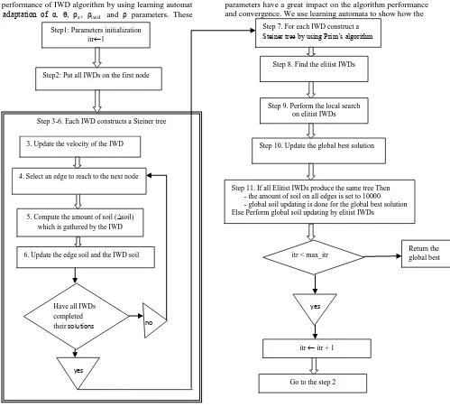
The flowchart of the EIWD algorithm is shown in Figure 2.
4.
USING LEARNING AUTOMATA FOR
PARAMETER ADAPTATION OF EIWD
ALGORITHM
Intelligent Water Drops algorithm has several parameters such as global soil updating parameter ρiwd, local soil updating parameter ρ, velocity updating parameters , av, bv and cv and
soil updating parameters , as, bs and cs. The efficiency of the
IWD algorithm is greatly dependent on tuning its parameters. Usually, the optimal (or near optimal) parameters are chosen by the trial-and-error procedure or using the past experience. As the number of trials necessary to fine-tune the parameters is usually quite high, it is often the case that limited time is
used for each algorithm run.
the performance of IWD algorithm by using learning automat for adaptation of α, , ρs, ρiwd and ρ parameters. These
[image:4.595.66.565.72.523.2]parameters have a great impact on the algorithm performance and convergence. We use learning automata to show how the
Fig 2: Flowchart of the EIWD algorithm for solving Steiner tree problem
state of the algorithm should influence the parameters. During the runs, the algorithm may learn what is the relation between the algorithm state, and the optimal parameter values.
4.1
Learning Automata
An automaton is a machine designed to automatically follow a predetermined sequence of operations or respond to encoded instructions. A finite number of actions can be performed in a random environment. When a specific action is performed, the environment provides a random response which is either favorable or unfavorable. The objective in the design of the automaton is to determine how the choice of the action at any stage should be guided by past actions and responses. Learning automata can be classified into two main families, fixed and variable structure learning automata.
The proposed algorithm is implemented with different kinds of learning automata. Simulation results show that the Krylov automaton produces better results than other fixed structure learning automata and variable structure learning automata. In [23] is shown that how we can choose the best automaton for parameter adaptation of ant colony optimization for solving
Steiner tree problem. In the following, we briefly describe Krylov automaton which we use in this paper.
4.2
Krylov Learning Automata
The Krylov automaton has 2N states and two actions. It keeps an account of the number of successes and failures received for each action. For favorable response the automaton moves deeper into the memory of the corresponding action and for unfavorable response moves out of it. The state transition graph of Krylov automaton is shown in Figure 3.
a. favorable response
b. unfavorable response
Fig 3: The state transition graph for Krylov automaton
1 2 3 N-1 N 2N 2N-1 N+3 N+2 N+1
1 2 N-1 N 2N 2N-1 N+2
0.5
0.5 0.5 0.5 0.5 0.5 0.5 N+1
Step 3-6. Each IWD constructs a Steiner tree
5. Compute the amount of soil (soil)
which is gathered by the IWD
6. Update the edge soil and the IWD soil
Have allIWDs
completed
their solutions
4. Select an edge to reach to the next node
3. Update the velocity of theIWD
no
yes
Step1: Parameters initialization
itr1
Step2: Put all IWDs on the first node
Step 8. Find the elitist IWDs
Step 9. Perform the local search on elitist IWDs
Step 10. Update the global best solution
Step 11. If all Elitist IWDs produce the same tree Then - the amount of soil on all edges is set to 10000 - global soil updating is done for the global best solution Else Perform global soil updating by elitist IWDs
Step 7. For each IWD construct a Steiner tree by using Prim’s algorithm
itr < max_itr
yes
itr itr + 1
Return the global best
[image:4.595.340.541.666.739.2]Table 1. Comparison of IWD and EIWD with other algorithms
Graph No.
Optimal
Cost |nodes| |Edges| |Terminals| SDG SPH ADH ACS NLA GA PSO IWD EIWD
1 82 50 63 9 0 0 0 0 0 0 0 0 0
2 83 50 63 13 84.3 0 0 0 0 0 0 0 0
3 138 50 63 25 1.45 0 0 0 0 0 0 0 0
4 59 50 100 9 8.43 5.08 5.08 2.7 0 0 0 0 0
5 61 50 100 13 4.92 0 0 0 0 0 0 0 0
6 122 50 100 25 4.92 3.28 1.64 1.8 0 0 0 0 0
7 111 75 94 13 0 0 0 0 0 0 0 0 0
8 104 75 94 19 0 0 0 0 0 0 0 0 0
9 220 75 94 38 27.2 0 0 0.05 0 0 0 0 0
10 86 75 150 13 3.95 4.65 4.65 3.84 0 0 0 0 0
11 88 75 150 19 2.27 2.27 2.27 1.59 1.8 0 0 0.23 0
12 174 75 150 38 0 0 0 0.11 0 0 0 0 0
13 165 100 125 17 6.06 7.88 2.24 0 4.2 0 0 0.61 0
14 235 100 125 25 1.28 2.55 0.43 0.09 0 0 0 0 0
15 318 100 125 50 2.20 0 0 0 0 0 0 0 0
16 127 100 200 17 7.87 3.15 0 0.16 1.2 0 0 0 0
17 131 100 200 25 34.5 3.82 3.05 1.22 1.3 0 0 0 0
18 218 100 200 50 4.59 1.83 0 1.42 0 0 0 0.46 0
4.3
Parameter Adaptation by Using Krylov
Automaton
To adjust IWD parameters we used 5 learning automata. Each automaton is used for setting one decision parameter. Legal values for decision parameters are as follows.
∝, θ ∈ 2,3,4 (12)
ρ ∈ −0.5, −0.6, −0.7, −0.8, −0.9 ρs∈ {1.5, 1.6, 1.7, 1.8, 1.9, 2 ,2.1 ,2.2}
ρiwd = {0.1, 0.2, 0.3, 0.4, 0.5, 0.6, 0.7, 0.8, 0.9}
The actions of an automaton are legal values of the correspond parameter. At the start of the algorithm, selected actions of learning automata (IWD parameters) and the depth associated with each action (N) are chosen randomly form the set of allowable values. At the beginning of each iteration of the IWD algorithm, each learning automaton selects one of its actions. The values of selected actions are used by all water drops to produce Steiner trees. At the end of the iteration, cost of the best-iteration tree is given to learning automata as the response of the environment. If the best-iteration tree cost is less than the global-best tree cost until this iteration, selected actions by each of the five automata are rewarded. Otherwise selected actions are penalized.
5.
Experimental results
In the first experiment, we ran the IWD and EIWD on the B-problem set from OR-library [24]. The results are the average date of 10 runs for each test instance with 50 iterations for each run. Table 1 compares the performance of the proposed algorithms with seven reported algorithms for building Steiner
tree in graphs while the details of DNH1, SPH2 and ADH3 have been illustrated in [16]. Ant colony optimization (ACS), learning automata approach (NLA) and particle swarm intelligence technique are described in [21], [25] and [19] respectively.
The format of Table 1 is as follows: The first column is used to express the graph number in B-problem set from Beasley. The second column gives the optimal cost of Steiner tree, the next three columns indicate the number of nodes, edges and terminals of each graph and other columns give relative error for each algorithm. The relative error criterion calculated as follows.
relative − error =C−Copt
Copt (13)
Where Copt is the optimal solution of a given problem and C is
the solution by a certain algorithm. In this experiment, we used trial and error procedure to select the best values for IWD parameters. These values are ∝= 3, θ = 3, ρ =
−0.9, ρs= 1.9 and ρiwd = 0.9.
Table 1 shows that EIWD gets better results compared to IWD. The EIWD obtained the optimal solution for all instances. Even though the IWD can’t succeed in obtaining the optimal solution on problems B11, B13 and B18, the relative error values are very small and the algorithm outperforms other algorithms expect for GA and PSO.In the second experiment, we compare the convergence speed of the best algorithms of the previous experiment. Table 2 shows the
1
Distance network heuristic
2
Shortest path heuristic
3
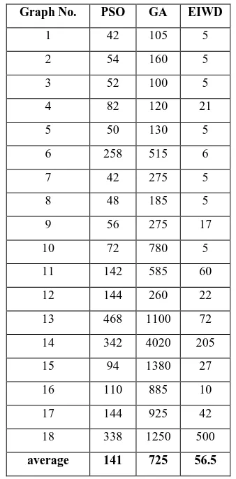
number of generated Steiner trees by GA and PSO before finding out the optimal tree. As can be seen, our proposed algorithm has much faster convergence speed than others. The EIWD generates average 57 trees to find the optimal solutions which is only 7% of the GA and 40% of the PSO. In conclusion, although GA and PSO find out the optimal solutions but they require excessive execution time especially for large size networks and it is not suitable for time limited applications such as real time multicasting.
Table 2. The number of trees generated by PSO, GA and EIWD.
Graph No. PSO GA EIWD
1 42 105 5
2 54 160 5
3 52 100 5
4 82 120 21
5 50 130 5
6 258 515 6
7 42 275 5
8 48 185 5
9 56 275 17
10 72 780 5
11 142 585 60
12 144 260 22
13 468 1100 72
14 342 4020 205
15 94 1380 27
16 110 885 10
17 144 925 42
18 338 1250 500
average 141 725 56.5
To determine the number of elitist IWDs (Ne), we ran EIWD algorithm with different number of elitist IWDs and calculate the average relative error on 18 test cases of OR-library. Figure 4 shows that the best value for Ne is 5. Thus, in all experiments we set Ne as 5.
Fig 4. Average relative error versus number of elitist IWDs
In the next experiment, we examine the effect of parameter adaptation on the performance of the EIWD algorithm. At first, we used trial and error procedure to find parameter setting that results in optimal trees for all test cases of
B-problem set. Then, we ran EIWD algorithm on C-B-problem set of OR-library by using these values and by using learning automata for parameter adaptation. C-problem set is a set of large and hard networks with 500 nodes in the OR-library. The results are average of 5 runs of the algorithms with 50 iterations in each run. Table 3 shows that using learning automata for parameter adaptation improve the performance of the algorithm. In fact, using learning automata causes that algorithms adapt better to the particular instance's characteristics. The proposed algorithm also obtained better results compared to genetic algorithm.
Table 3: The effect of learning automata for parameter adaptation
Graph No.
Optimal Cost
GA EIWD
With constant parameters
EIWD With parameter adaptation
1 85 0 0 0
2 144 0 0 0
3 754 0.50 0.13 0.05
4 1079 0.44 0.18 0.17
5 1579 0.10 0.19 0.09
6 55 0 0 0
7 102 0 0 0
8 509 1.14 1.18 0.63
9 707 1.27 1.41 1.27
10 1093 0.36 0.64 0.64
11 32 0 0 0
12 46 0.43 0 0
13 258 1.36 1.16 1.16
14 323 1.42 1.55 1.55
15 556 1.04 0.54 0.54
16 11 2.73 0 0
17 18 1.11 4.44 1.11
18 113 4.78 6.19 4.78
19 146 5 7.53 5.14
20 267 2.02 0.75 0.22
In summary, EIWD algorithm provides an acceptable trade off between solution quality and solution time.
6.
CONCLUSION AND FUTURE WORKS
In this paper, we extended the IWD algorithm for solving Steiner tree problem in graphs. In our extended version, at the end of each iteration instead of the best IWD of the iteration, prescribed numbers of the best IWDs (called elitist IWDs) perform global soil updating. In addition, to overcome the problem of premature convergence, when all elitist IWDs produce the same tree the amount of soil on all edges of the graph is set to the initial value and then the global soil updating is done for the best resulted tree.
To assess the performance of the proposed algorithm, the B-problem set of the OR-library is used. Experimental results show that our algorithm is able to find optimal solutions for 0
0.02 0.04 0.06 0.08
1 2 3 4 5
av
e
ra
ge
o
f
re
la
ti
ve
e
rr
o
r
[image:6.595.319.538.215.595.2] [image:6.595.53.263.593.697.2]all test instances in B-problem set from Beasley. Compare to GA and PSO which are able to obtain optimal solutions for all test cases in the OR-library, the proposed algorithm has much faster convergence speed. This indicates that the EIWD algorithm is an efficient approach in real time multicast routing.
In addition, we improved the performance of EIWD algorithm for solving Steiner tree problem by hybridizing it with learning automata for parameter adaptation. Experimental results on C-problem set of the OR-library showed that this hybrid algorithm achieved better results.
Adapting the EIWD algorithm to Euclidian and Rectilinear Steiner tree problems and other variations of the problem such as Steiner forest or prize collecting Steiner forest problem, will be an interesting future research field. In addition, the EIWD algorithm has quick convergence that can be advantageous for time constrained problems. This future helps to extend proposed algorithm for solving dynamic Steiner tree problem.
7.
REFERENCES
[1] Li, K., Shen, C., Jaikaeo, C. and Sridhara, V. 2008. Ant-based Distributed Constrained Steiner Tree Algorithm for Jointly Conserving Energy and Bounding Delay in Ad hoc Multicast Routing, ACM Transactions on Autonomous and Adaptive Systems, 3, 1.
[2] Hu, X., Zhang, J. and Zhang, L. 2009. Swarm Intelligence Inspired Multicast Routing: An Ant Colony Optimization Approach, EvoWorkshops, 51-60.
[3] Shah-Hosseini, H. 2007. Problem Solving by Intelligent Water Drops, in Proceedings of IEEE Congress on Evolutionary Computation, Singapore, 3226-3231. [4] Shah-Hosseini, H. 2009. The Intelligent Water Drops
Algorithm: A Nature-Inspired Swarm-Based Optimization Algorithm, International Journal of Bio-Inspired Computation, 1 , 71-79.
[5] Shah-Hosseini, H. 2009. Optimization with the Nature-Inspired Intelligent Water Drops Algorithm, In Santos, W.P.D. ed. Evolutionary computation. Tech, Vienna, Austria, 297-320.
[6] Shah-Hosseini, H. 2011. An Intelligent Water Drop Algorithm for Solving Economic Load Dispatch Problem, International Journal of Electrical and Electronics Engineering, 5, 1.
[7] Hougardy, S., and Promel, H. J. 1999. A 1.598 Approximation Algorithm for the Steiner Problem in Graphs, ACM-SIAM Symposium on Discrete Algorithm, USA, 448-453, 1999.
[8] Laarhoven, V. and William, J. 2010. Exact and Heuristic Algorithms for the Euclidean Steiner Tree Problem, PhD thesis., University of Iowa.
[9] Cormen, T. H., Leiserson, C. E., Rivest, R.L., and Stein, C. (2001), Introduction to Algorithms, 2nd edn. MIT Press, Cambridge.
[10]Karp, R. M. 1972. Reducibility among combinatorial problems, In Complexity of Computer Computation, Plenum Press, New York, 8-103.
[11]Garey, M. R., Graham, R. L. and Johnson, D.S. 1977. The Complexity of Computing Steiner Minimal Trees, SIAM Journal of Applied Mathematics, 32, 4, 835-859. [12]Garey, M.R. and Johnson, D.S. 1977. The Rectilinear
Steiner Tree Problem is NP-complete, SIAM Journal on Applied Mathematics, 32, 4, 826-834.
[13]Esbensen, H. 1995. Computing Near-Optimal Solutions to the Steiner Problem in a Graph Using a Genetic Algorithm, Networks, 26, 173-185.
[14]Robins, G. and Zelikovski, A. 2000. Improved Steiner Tree Approximation in Graphs, In Proc. 11th ACM-SIAM Symposium on Discrete Algorithms, pp. 770-779, 2000.
[15]Diane, M., and Plesnik, J. 1999. Three New Heuristics for the Steiner Problem in Graphs, Acta Math., LX, 105-121.
[16] Rayward-smith, V. J., and Clare, A. 1986. On Finding
Steiner vertices, Networks, 16, 283-294.
[17] Kapsalis, A., Rayward-smith, V. J., and Smith, J. D.
1993. Solving the Graphical Steiner Tree Problem Using Genetic Algorithms, Journal of the Operational Research Society, 44 , 397-406.
[18] Ding, S., and Ishii, N. 1995. An Online Genetic
Algorithm for Dynamic Steiner Tree Problem, Symposium on Computational Geometry, 337-343.
[19] Zhan, Z., and Zhang, J. 2009. Discrete Particle Swarm
Optimization for Multiple Destination Routing Problems, In Proceedings of EvoWorkshops, 117-122.
[20] Ma, X. and Liu, Q. 2010. A Particle Swarm Optimization
for Steiner Tree Problem, In Sixth International Conference on Natural Computation, ICNC 2010, 2561-2565.
[21] Tashakori, M., Adibi, P., Jahanian, A. and Norallah, A.
(2004), ‘Solving Dynamic Steiner Tree Problem by Using Ant Colony System’, in 9th Annual Conference of Computer Society Of Iran, Tehran, Iran.
[22] Meybodi, M. R., and Beigy, H. 2002. A Note on
Learning Automata Based Schemes for Adaptation of BP Parameters, Journal of Neurocomputing, 48, 957-974.
[23] Noferesti, S., and Rajaei, M. 2011. A Hybrid Algorithm
Based on Ant Colony System and Learning Automata for Solving Steiner Tree Problem, International Journal of Applied Mathematics and Statistics, 22.
[24] Beasley, J. E. 1990. OR-Library: Distributing Test
Problems by Electronic Mail, Operational Research. SOC., 41 ,11, 1096-1072.
![Fig 1: An example of the Steiner tree in graph The Steiner tree problem is NP-hard even in Euclidean or rectilinear metrics [10-12]](https://thumb-us.123doks.com/thumbv2/123dok_us/8121906.794441/2.595.104.249.181.302/example-steiner-graph-steiner-problem-euclidean-rectilinear-metrics.webp)