http://dx.doi.org/10.4236/jsea.2014.710076
Combining Geographic Information Systems
for Transportation and Mixed Integer Linear
Programming in Facility Location-Allocation
Problems
Silvia Maria Santana Mapa1, Renato da Silva Lima2
1Federal Office for Education, Science and Technology of Minas Gerais, Congonhas, Brazil 2Federal University of Itajuba, Industrial Engineering and Management Institute, Itajubá, Brazil
Email: [email protected], [email protected]
Received 6July 2014; revised 3August 2014; accepted 1September 2014
Copyright © 2014 by authors and Scientific Research Publishing Inc.
This work is licensed under the Creative Commons Attribution International License (CC BY). http://creativecommons.org/licenses/by/4.0/
Abstract
In this study, we aimed to assess the solution quality for location-allocation problems from facili-ties generated by the software TransCAD®, a Geographic Information System for Transportation (GIS-T). Such facilities were obtained after using two routines together: Facility Location and Transportation Problem, when compared with optimal solutions from exact mathematical models, based on Mixed Integer Linear Programming (MILP), developed externally for the GIS. The models were applied to three simulations: the first one proposes opening factories and customer alloca-tion in the state of São Paulo, Brazil; the second involves a wholesaler and a study of locaalloca-tion and allocation of distribution centres for retail customers; and the third one involves the location of day-care centers and allocation of demand (0 - 3 years old children). The results showed that when considering facility capacity, the MILP optimising model presents results up to 37% better than the GIS and proposes different locations to open new facilities.
Keywords
Geographic Information Systems for Transportation, Location-Allocation Problems, Mixed Integer Linear Programming, Transportation, TransCAD®
1. Introduction
prob-lem complexity increases, location studies require new information technologies, which permit systems to be treated with effective integration [1]. Approximate facility location models have been proposed by using tools to help them in space, especially when a geographically referenced database is available. In this case, Geographic Information Systems (GIS) are vital for data collection and data analysis, since they incorporate a sophisticated graphical interface into a geographically referenced database, thus becoming powerful tools for spatial analysis and planning [2]. Geographic Information Systems for Transportation (GIS-T) is a special class of GIS, being used for transportation planning and operating. Among its many features, it has sections for facility location. Nothing more natural, thus, than using GIS-T tools to study the best locations for public or private facilities— e.g. factories, distribution centres (DCs), schools or day-care centers—and the best distribution of these units to customers trying to reduce or offset the costs of displacement and/or transportation.
A variety of software programs may be used to aid in location problems. Most of them, however, end up working as a “black box”, i.e. their solution methods are not clear, usually leading users to make assumptions and believe in the efficiency of such solutions. From previous experiments performed in the location-allocation modules of TransCAD®, a commercial GIS-T package, it was verified that it solves problems, however indi-rectly within two steps. The first step includes the Facility Location routine, which identifies the best facility lo-cations (proposing entering new units or closing existing ones, or both), and proceeds to allocate between supply and demand, but without considering the full operation for the facilities. To enforce such restrictions to maxi-mum capacity, a second step is necessary in which the solution of the Facility Location routine (FL routine) is submitted to the Transportation Problem routine (TP routine). Thus, the solution of the FL routine becomes the input of the TP routine, which will reallocate the supply to demand at the discretion of maximum capacity for facilities. However, this second routine no longer admits the opening or closing facilities previously generated by the FL routine, being pre-conditioned to its initial configuration. Such factor can also clearly compromise the quality of the final solution, since the choice of opening and/or closing of new facilities is certainly subject to their respective capabilities. Additionally, we must consider both routines work with heuristic algorithms in finding solutions. Consequently, there is no guarantee that the solution found after using the routines is the op-timal solution, and one would only know for sure by resolving the problem using an optimisation algorithm.
This is the starting point for this study, in which we aimed at assessing the solution quality for location-allo- cation problems from facilities generated by TransCAD®. Such facilities were obtained after using the FL and TP routines together, when compared with optimal solutions from exact mathematical model, based on MILP and developed outside of the GIS. The MILP model can locate and allocate facilities to customers, while simul-taneously obeying bounds of maximum capacity for such facilities, unlike the use of GIS combined routines.
For this study research methodology, classified as modelling and simulation, for both models, i.e. GIS and MILP, we applied three simulations (s1, s2, s3) within different complexity levels. For s1: factory, allocation opening and customer allocation within 18 major São Paulo municipalities. For s2: study of location on distribu-tion centres from wholesalers and allocadistribu-tion of their retail customers in the Brazilian states of Minas Gerais and São Paulo. For s3: day-care center location and demand allocation (for children from zero to three years old) in the city of São Carlos (state of São Paulo, Brazil). Thus, the results from the MILP and GIS models were com-pared and assessed. This study is structured as follows: Section 2 presents considerations on the paper’s theo-retical analysis; Section 3 demonstrates the chosen research methodology; Section 4 exhibits the three tions based on the research methodology of Section 3; Section 5 gives a general assessment of the three simula-tions; and Section 6 offers conclusions for this study along with bibliographic references.
2. Theoretical Analysis
2.1. Facility Location
Facility location problems involve choosing the best location for one or more facilities within a set of possible locations, to provide a high level of customer service, reduce operating costs, or increase profits. Based on [3], a potential optimum solution is sought, which will cut down total facility and transportation cost.
models (Table 1).
Applications for facility location problems occur in both the private and public sectors, focused on being as close as possible to demand, in order to reduce transport costs, increase the coverage area and the level of de-mand accessibility or totally reduce the facility costs, either by choosing a location because of the financial cost, or the quantity of facilities to be established.
2.2. Geographic Information Systems (GIS)
According to [6], GIS can be defined as an organised collection of hardware, software, skilled personnel, and geographic data, in order to manage a database, making the insertion, storage, handling, removal, update, as-sessment, and data visualization, both spatial and non-spatial (attribute data), functioning as a valuable tool in planning and management studies. Understanding GIS only as software is to exclude the crucial role it can play in a broad process of decision making. According to [2], since the 1990s there has been a vast and growing terest in GIS in the academic world, software companies, and among professionals, as a consequence of in-creased processing capacity, reduced microcomputer costs and inin-creased availability of digital cartographic da-tabases. Due to the specific requirements for transport and the adoption of information technology in this area, researchers have increased their efforts to improve the existing GIS approach. Thus, they enable such effort for transportation studies, giving rise to so-called GIS-T.
According to [1], six interrelated factors stand out for the growing use of GIS: 1) there is a range of GIS soft-ware available from commercial vendors and universities; 2) increasing capacity of computers to store and re-trieve vast amounts of data within reasonable time and cost parameters; 3) more sophisticated and faster printers to produce high resolution and quality outputs; 4) greater availability of spatial data from affordable private companies and government agencies; 5) expanding the use of remote sensing, which requires systems that can deal with a lot of data; and 6) the emergence of Global Positioning System (GPS), which facilitate collecting spatial data at relatively low cost and high accuracy.
2.3. Applying GIS to Facility Location Problems
As cited by [7], “the combination of GIS and location science is at the forefront of advances in spatial analysis capabilities, offering substantial potential for continued and sustained theoretical and empirical evolution”. According to [8], several studies have been developed in logistics, facility location and vehicle routing by using a GIS, at times combined with other mathematical techniques, applied to both the public and private sectors. In the case of the private sector, the main objective is to minimize logistics costs. For example, for industries, wholesalers, retailers, and distributors to decide the best place to install a unit (or a production plant, a shop, a storage or DC) one should always take into consideration the market positioning of consumers and suppliers, availability of infrastructure, manpower and various other factors affecting production.
Reference [9]presents a new class of facility location-allocation problems to consider the optimal location of two types of installations, static and transportation, to meet a set region with minimum cost. To illustrate this, consider the location of hospitals as a static installation and location of ambulances as transportation facilities.
Table 1. Classification of location problems (Owen et al., 1998).
Problem Description
p-median model
Locate p facilities at the vertices of a network and allocate the demand to these facilities to reduce the distance travelled. If the facilities are not capacitated and p is fixed, then it is a p-median problem, in which all vertices are assigned to their closest facility. If p is a decision variable and the facilities are capacitated or non-capacitated, it is set as a Capacitated or Non-Capacitated Facility Location problem, respectively. These models are particularly relevant for the design of logistics and load allocation.
Cover sets
Cover sets are based on distance or maximum acceptable trip time, seeking to lessen the quantity of facilities to ensure some level of client coverage. It assumes a finite set of locations and is typically associated with a fixed budget. It is widely used to locate public services, e.g. health centres, post offices, libraries or schools.
Model centres
The location of the transportation facilities is dependent on location of static facilities and demand objects. The authors proposed a new GIS platform combined with a heuristic algorithm, customised to solve the problem. Further, the results are available in a user-friendly graphical interface, using thus many resources in developing and applying GIS in location models. Reference [10]developed a model based on GIS for the location of wind, solar, and hydropower energy systems, related to the temporal characteristics of supply and demand worldwide, focusing on locating sources of energy to meet 21st century global demand.
Other examples of GIS application in studies of location can be seen in the literature, such as: Reference [11] describes the development of a planning procedure based on GIS to assist decision makers in site selection when various accessibility criteria are considered. Reference [12], who integrated ArcGIS® with an expert system to assist in the allocation of bank branches; Reference [13] developed a heuristic method integrated with GIS loca-tion-allocation problems for maximum coverage and location of the p-median; Reference [14] applied multi- criteria decision analysis in locating power plants using GIS-T; Reference [15] performed a study on current lo-cation and a proposed relolo-cation of state schools in Brazilian municipalities; Reference [2] studied the lolo-cation of day-care centers and health clinics in urban areas using GIS location models; Reference [16] conducted a study to allocate sewage treatment plants and landfills; Reference [17] located cross-docking centres for a phar-maceutical products network; Reference [18] studied how to allocate consolidation terminals for the less-than- truckload trucking industry in Brazil; Reference [19] developed a manufacturing plants or deposits (or both) global-scale model for transnational corporations.
According to [8], GIS capacity rises considerably when it is combined with the use of Operational Research techniques. Reference [20] suggest that the use of exact programming models that use the branch-and-bound al-gorithm are limited to finding a global solution, effectively optimal to problems with up to 150 nodes on the network. A branch-and-bound algorithm is a tree search method with intelligent enumeration for candidate solu-tions to the optimal solution of a problem by performing successive partisolu-tions of the space of solusolu-tions and cut-ting the search tree by considering limits calculated along the enumeration. The calculation of bounds for the value of the optimal solution is a key part of a branch-and-bound algorithm, since it is used to limit the growth of the tree. Using more robust techniques such as Lagrangian relaxation with optimisation subgradient, increases the ability to handle more complex optimisation problems, roughly from 800 to 900 nodes on the network. Therefore, exact algorithms are only used to solve problems with a restricted number of variables and con-straints.
3. Research Methodology
This mathematical model is classified as static and deterministic, resolved by a variant from the p-median prob-lem, focusing on finding the location of p-facilities, since the total distance between supply and demand centres should be minimised while simultaneously allocating the flows between facilities and customers. An interaction between the GIS and external mathematical model, based on MILP, is proposed which will occur during data input and output. According to [20]and [21], the MILP is the most widely used mathematical method for solv-ing location problems formulated by the p-median method, leading to the optimal solution of the problem.
This research sought to assess the solution quality generated by GIS software, in the combined FL and TP routines, when compared to the optimal solution from the MILP model. Even if the GIS mathematical solution quality is bad in a pessimistic assumption, its great help in data collection and solution finding and presentation phases cannot be denied , such as by using its tools for generating graphics and thematic maps etc. According to [1], exporting data from GIS is not difficult, and will serve as input to another location model, external to GIS, which will solve the problem proposed, and then import the results back to GIS to create the graphical results in map form. The MILP model was implemented by using the optimisation software LINGO®, version 7.0, with interface in an MS Excel® spreadsheet, as detailed in the following equations:
Function objective:
, ,
min i j i j j
i j
fo=
∑∑
C ∗X ∗d (1)Subject to:
i i
z = p
, ,
i j i
X ≤z ∀i j (3)
, 1
i j i
X = ∀j
∑
(4),
j i j i i
j
d ∗X ≤m∗z ∀i
∑
(5)( )
0,1i
z ∈ ∀i (6)
, ,
i j
X ∈Z+ ∀i j (7) where:
,
i j
X : is the matrix solution. It indicates the percentage of demand j satisfied by i; ,
i j
C : is the cost matrix, represented by the minimum distances between points i and j; i
z : is a binary vector, indicating which facilities are opened. If zi=1, the facility i is opened. Otherwise,
if 0zi= , then the facility i is not in operation;
j
d : vector that stores customers’ demands j; i
m: input parameter that defines the maximum capacity of facility i;
p: input parameter that specifies the amount of facilities to be opened.
Equation (1) represents the objective function of the model to decrease shipping costs, depending on the dis-tances between points i (set of facilities) and j (set of customers), weighted by the percentage of demands, as well as the objective function in the GIS, for comparison of results generated between the two models. With respect to restrictions, it is worthy to note that Equation (2) is the constraint that indicates the number of facili-ties to be opened, equivalent to the number p; (3) represents the restriction for opening facilities, i.e. if i is not in operation
(
0zi=)
, the allocation of demand to the facility must be zero; (4) is the restriction of demand coverage, in which all customers should have the total of their demands met; (5) is the restriction of upper bound for capacity of facilities to be opened; (6) makes the output vector zi a binary vector; and (7) makes the solu-tion matrix Xi j, an integer matrix.The research methodology used in the research can be classified as scientific research being applied, follow-ing a quantitative approach with exploratory objectives and usfollow-ing modellfollow-ing and simulation as a technical pro-cedure [22]. It was implemented in three simulations, according to the GIS and MILP model, involving different complexity levels. In general, the location-allocation problem will approach how to decrease transportation costs in a logistics network, in which the supply (or demand) centres shall fully meet the demands of customers, whether or not subject to the restriction of the upper bound for capacity of facilities. To support the calculations of the models, a computer with an AMD Sempron 2600, 1.83 GHz and 512 MB of RAM was used, operating under the operating system Microsoft Windows XP Professional.
4. Simulation
4.1. Simulation I—Locating Factories
The problem proposed for this simulation is to perform the location and allocation between supply points (plants) and demand (customers) in São Paulo, including 18 of its major cities. To find the points of supply, the choice will be given in a discrete space, which will include all 18 municipalities as candidates for opening facilities for both models, GIS and MILP.
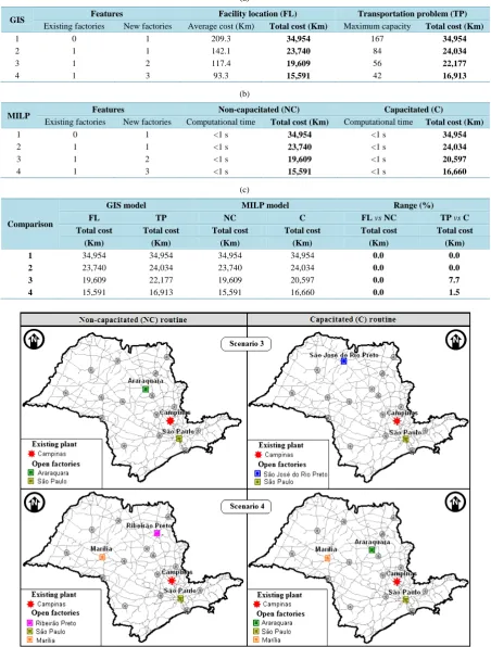
The objective function enabled in all scenarios was to decrease the average transport service cost. The numeri-cal results of the scenarios generated by the GIS model for the FL and TP routines, can be found in Table 2(a). From the assessment of Table 2(a), one can realise that the values of transport service Total Cost decreases as the number of factories increase, so that as customers get closer and in turn reducing transport costs. It is hugely im-portant to assess solutions generated by the TP routine, which relocated demands according to the maximum ca-pacity of factories, enabling fragmentation (customers/cities may be served by more than one factory). Thus, it is easy to notice an increase in the value of Total Cost (in scenarios 2, 3, 4), in which all scenarios are compared with respective solution generated by FL routine. This increase is a consequence of the maximum capacity limits imposed on the facilities offered by the TP routine that, once reached, can no longer allocate demand to that in-stallation. The computer processing time was less than one second in all situations.
To draw a comparison between the GIS and MILP models, the same scenario used in the GIS model was simulated in the MILP model. The MILP model can also solve the problem without considering plant capacity, which was called non-capacitated (NC) routine, running exactly as the FL routine of GIS. When you consider these capabilities, the model was called a capacitated (C) routine, making the location and allocation of facilities to their clients and checking the limits of a maximum capacity of these facilities simultaneously, unlike the GIS. Thus, for comparison, the C/MILP routine corresponds to TP/GIS routine, stressing that the TP output of GIS ac-tually means the combined use of the FL and TP routines. The quantitative results of the MILP model are pre-sented in Table 2(b).
Figure 1 presents the spatial results for scenarios 3 and 4, where plant location solutions proposed by NC and C routines were different. Comparing the solutions generated by the GIS and MILP, it can be seen that at first the two models behave similarly. The solutions produced by FL/GIS were equal to those generated by the NC/MILP in all scenarios. This can be seen by comparing the values of the total cost, available in Table 2(c), for the FL/GIS routine and NC/MILP routine.
4.2. Simulation II—Locating Wholesale Distribution Centres
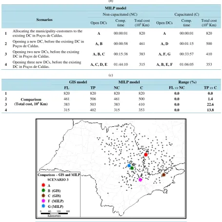
The objective here is to locate DCs for a wholesale company. The company has only one DC located in the city Poços de Caldas, in southern Minas Gerais, Brazil. The wholesaler has a total of roughly 12,000 customers, 30% of them located in southern Minas Gerais and 70% distributed in the São Paulo countryside, concentrated in Vale do Paraíba and the regions of Campinas and Ribeirão Preto. To simplify the problem, all customers within the same municipality were grouped and had their demands combined into a single point, so the demand points were municipalities connected by motorways. There has been, thus, a total of 311 municipality-customers, each with its own geographical location and total demand. The quantity of municipality candidates to have a DC was restricted to 150 for the GIS and MILP models, chosen among those municipality-customers with the highest demand val-ues (89% of total demand). It was the first significant restriction of the MILP model. Despite the software Lingo not imposing limits on the number of problem variables and constraints (only the processing time that rises expo-nentially), the Excel spreadsheet interfaced with Lingo has a maximum number of columns (256) to store the cost matrix (distances) among the municipality-customers and candidates to DC location.
The criterion to generate the scenarios was the same as in simulation I. Table 3(a) shows its numerical results. The minimum total cost of transport with the current DC (scenario 1) would be 820 × 106 Km. When opening a new DC in the TP/GIS model (scenario 2), the wholesaler may reduce their transportation costs by 38.3% when compared to scenario 1. Table 3(b) presents the MILP model results for the same scenarios. In addition to the Total Cost variable, Table 3(b) also shows the computational processing time, which rises with the number of DCs to be localised. In all scenarios that included the opening of new DCs (2, 3, 4), the C/MILP routine and NC/MILP routine indicated different cities to open such new DCs. The comparison for GIS and MILP model is shown in Table 3(c).
Table 2. Results for simulation I.
(a)
GIS Features Facility location (FL) Transportation problem (TP)
Existing factories New factories Average cost (Km) Total cost (Km) Maximum capacity Total cost (Km)
1 0 1 209.3 34,954 167 34,954
2 1 1 142.1 23,740 84 24,034
3 1 2 117.4 19,609 56 22,177
4 1 3 93.3 15,591 42 16,913
(b)
MILP Features Non-capacitated (NC) Capacitated (C)
Existing factories New factories Computational time Total cost (Km) Computational time Total cost (Km)
1 0 1 <1 s 34,954 <1 s 34,954
2 1 1 <1 s 23,740 <1 s 24,034
3 1 2 <1 s 19,609 <1 s 20,597
4 1 3 <1 s 15,591 <1 s 16,660
(c)
Comparison
GIS model MILP model Range (%)
FL TP NC C FL vs NC TPvs C
Total cost Total cost Total cost Total cost Total cost Total cost
(Km) (Km) (Km) (Km) (Km) (Km)
1 34,954 34,954 34,954 34,954 0.0 0.0
2 23,740 24,034 23,740 24,034 0.0 0.0
3 19,609 22,177 19,609 20,597 0.0 7.7
4 15,591 16,913 15,591 16,660 0.0 1.5
Table 3. Results for simulation II.
(a)
GIS model
Scenarios
Facility location (FL) Transportation problem (TP)
Open DCs Average cost (Km)
Total cost (106 Km)
Capabilities (Kg)
Total cost (106 Km)
1 Allocating the municipality-customers to the
existing DC in Poços de Caldas. A 212 820 3,861,936 820
2 Opening a new DC, before the existing DC in
Poços de Caldas. A, B 121 461 1,930,968 506
3 Opening two new DCs, before the existing DC
in Poços de Caldas. A, B, C 101 383 1,287,312 503
4 Opening three new DCs, before the existing
DC in Poços de Caldas. A, C, D, E 83 315 965,484 402
(b)
MILP model
Scenarios
Non-capacitated (NC) Capacitated (C)
Open DCs Comp.
time
Total cost
(106 Km) Open DCs
Comp. time
Total cost (106 Km)
1 Allocating the municipality-customers to the existing DC in Poços de Caldas. A 00:00:01 820 A 00:00:01 820
2 Opening a new DC, before the existing DC in Poços de Caldas. A, B 00:00:58 461 A, D 00:01:15 500
3 Opening two new DCs, before the existing
DC in Poços de Caldas. A, B, C 00:15:38 383 A, F, G 00:33:57 410
4 Opening three new DCs, before the existing
DC in Poços de Caldas. A, C, D, E 01:44:10 315 A, B, E, F 01:06:05 353
(c)
GIS model MILP model Range (%)
FL TP NC C FL vs NC TPvsC
1
Comparison (Total cost, 106 Km)
820 820 820 820 0.0 0.0
2 461 506 461 500 0.0 1.4
3 383 503 383 410 0.0 22.6
[image:8.595.85.541.257.712.2]4 315 402 315 353 0.0 13.8
4.3. Simulation III—Locating Day-Care Centers
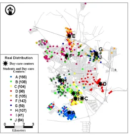
This simulation was based on locating public day-care centers and its demand allocation, i.e. children aged from zero to three years old, located in São Carlos city, in the state of São Paulo, Brazil. Data from the Mu-nicipal Education Office were used in a geo-referenced GIS file with the city’s transport network. These data correspond mainly to address and school attended by all students from public day-care centers (a total of 1014 students), distributed in 10 existing day-care centers (data from 2000).
The first step is to assess the real location and allocation of students and day-care centers. To do so, GIS thematic maps were used, in which students who attend the same day-care center are identified by a same colour. The bad distribution is easily identified by a visual assessment of Figure 3, in which the day-care centers appear identified by a single symbol, using the letters from A to J to distinguish them. In the map’s legend, every day-care center is associated with the number of students enrolled. From information obtained in the real situation assessment, different location scenarios and allocation among day-care centers and stu-dents have been proposed, seeking to concentrate more stustu-dents living by day-care center they attend. The scenarios was named as Real (real locations and allocations between students and day-care centers), Sce-nario 1 (reallocation of students for the ten-existing day-care centers), Scenario 2 (ten-existing day-care centers, opening a new unit), Scenario 3 (ten-existing day-care centers, opening two new units) and Scenario
4 (closing one of the ten day-care centers and opening a new unit).
[image:9.595.183.447.435.710.2]For scenario 1, the capacity limits imposed on each of the day-care centers for the TP routine were established as the number of students actually enrolled in a specific day-care center at the time of collection and data analy-sis. By streamlining, the lack or excess of vacancies was not considered, since the aim is only to compare the GIS and MILP model. Thus, the same parameters in both models were maintained. For scenarios 2 and 3, in which we proposed to open new day-care centers, the capacity of the new units was established as 10% from the total demand of students (101 from 1014 students enrolled), lessening the capacity for existing day-care centers. In scenario 4, the supply capacity for closed day-care centers was reallocated to the new unit opened by the model. Relatively few candidates for locations were chosen by using the location of equidistant points (0.7 Km), covering the entire city for a total of 120 points. Added to the ten-existing day-care centers, there are 130 candi-dates, a set used for both models (GIS and MILP). Once again, the processing capacity of the MILP exact model was limiting for the number of candidates considered.
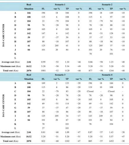
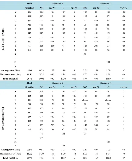
The GIS model results are shown in Table 4. Based on mean, maximum and total cost, one can see that all the simulated scenarios showed better results than the Real situation, with reductions of up to 60%. A simple real-location of students in the existing model (scenario 1) would lead to reductions of 50% in transportation costs.
[image:10.595.93.539.225.726.2]The MILP model results are presented in Table 5. The results are quite similar to the GIS model in quantita-tive terms, with significant reductions in displacement costs for the real situation. The most significant finding, however, is that in scenarios 2, 3, 4 the NC routine and C routine of the MILP model generated different loca-tions within the same scenario, i.e. when the restriction to maximum capacity is imposed on the model, location solutions for day-care centers, and consequently the allocation of students, are different. For example, in sce-nario 2 of the NC model, the day-care center to be opened would be letter K; and for C model would be letter M. The highest computational processing was nearly 2 hours in scenario 3 capacitated (01:52:14).
Table 4. Results for the GIS model.
Real Scenario 1 Scenario 2
Situation FL var % TP var % FL var % TP var %
DAY
-CA
RE
CE
NT
E
R
A 166 196 18 166 0 196 18 149 −10
B 108 115 6 108 0 115 6 97 −10
C 104 22 −79 104 0 22 −79 94 −10
D 98 78 −20 98 0 78 −20 88 −10
E 105 105 0 105 0 105 0 95 −10
F 142 147 4 142 0 69 −51 128 −10
G 59 37 −37 59 0 37 −37 53 −10
H 107 88 −18 107 0 88 −18 96 −10
I 41 125 205 41 0 125 205 37 −10
J 84 101 20 84 0 101 20 76 −10
K 78 101
L
Average cost (Km) 2.04 0.99 −52 1.10 −46 0.86 −58 1.23 −40
Maximum cost (Km) 10.52 5.28 −50 5.34 −49 5.20 −51 5.20 −51
Total cost (Km) 2070 1001 −52 1120 −46 877 −58 1244 −40
Real Scenario 3 Scenario 4
Situation FL var % TP var % FL var % TP var %
DAY
-CA
RE
CE
NT
E
R
A 166 169 2 133 −20 196 18 166 0
B 108 115 6 86 −20 119 10 108 0
C 104 22 −79 83 −20 Closed - Closed -
D 98 78 −20 78 −20 78 −20 98 0
E 105 105 0 84 −20 105 0 105 0
F 142 69 −51 114 −20 69 −51 142 0
G 59 37 −37 47 −20 37 −37 59 0
H 107 88 −18 86 −20 88 −18 107 0
I 41 125 205 34 −17 143 249 41 0
J 84 101 20 67 −20 101 20 84 0
K 78 101 78 104
L 27 101
Average cost (Km) 2.04 0.81 −60 1.09 −47 0.87 −57 1.43 −30
Maximum cost (Km) 10.52 5.20 −51 5.20 −51 5.20 −51 5.57 −47
Table 5. Results for the MILP model.
Real Scenario 1 Scenario 2
Situation NC var % C var % NC var % C var %
DAY
-CARE
CE
NT
E
R
A 166 196 18 166 0 196 18 149 −10
B 108 115 6 108 0 115 6 97 −10
C 104 22 −79 104 0 22 −79 94 −10
D 98 78 −20 98 0 78 −20 88 −10
E 105 105 0 105 0 105 0 95 −10
F 142 147 4 142 0 69 −51 128 −10
G 59 37 −37 59 0 37 −37 53 −10
H 107 88 −18 107 0 88 −18 96 −10
I 41 125 205 41 0 125 205 37 −10
J 84 101 20 84 0 101 20 76 −10
K 78
L
M 101
N
Average cost (Km) 2.04 0.99 −52 1.10 −46 0.86 −58 1.08 −47
Maximum cost (Km) 10.52 5.28 −50 5.34 −49 5.20 −51 5.28 −50
Total cost (Km) 2070 1001 −52 1120 −46 877 −58 1095 −47
Real Scenario 3 Scenario 4
Situation NC var % C var % NC var % C var %
DAY
-CARE
CE
NT
E
R
A 166 169 2 133 −20 196 18 166 0
B 108 115 6 86 −20 119 10 108 0
C 104 22 −79 83 −20 closed - closed -
D 98 78 −20 78 −20 78 −20 98 0
E 105 105 0 84 −20 105 0 105 0
F 142 69 −51 114 −20 69 −51 142 0
G 59 37 −37 47 −20 37 −37 59 0
H 107 88 −18 86 −20 88 −18 107 0
I 41 125 205 34 −17 143 249 41 0
J 84 101 20 67 −20 101 20 84 0
K 78 101 78
L 27
M 104
N 101
Average cost (Km) 2.04 0.81 −60 1.01 −50 0.87 −57 1.05 −49
Maximum cost (Km) 10.52 5.20 −51 5.20 −51 5.20 −51 5.34 −49
Total cost (Km) 2070 822 −60 1027 −50 885 −57 1063 −49
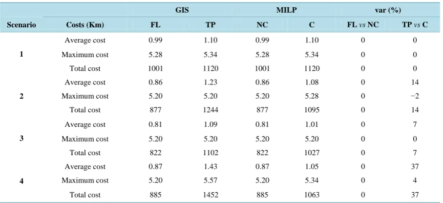
Table 6. Comparing the GIS and MILP models.
GIS MILP var (%)
Scenario Costs (Km) FL TP NC C FL vs NC TP vsC
1
Average cost 0.99 1.10 0.99 1.10 0 0
Maximum cost 5.28 5.34 5.28 5.34 0 0
Total cost 1001 1120 1001 1120 0 0
2
Average cost 0.86 1.23 0.86 1.08 0 14
Maximum cost 5.20 5.20 5.20 5.28 0 −2
Total cost 877 1244 877 1095 0 14
3
Average cost 0.81 1.09 0.81 1.01 0 7
Maximum cost 5.20 5.20 5.20 5.20 0 0
Total cost 822 1102 822 1027 0 7
4
Average cost 0.87 1.43 0.87 1.05 0 37
Maximum cost 5.20 5.57 5.20 5.34 0 4
Total cost 885 1452 885 1063 0 37
scenarios, where opening or closing (or both) of new units was proposed. In scenario 4, for example, the GIS model located the day-care center K to the north; and MILP model located day-care center M to the south with 37% lower cost.
5. General Assessment for the Results
It should be stressed here that a heuristic procedure is associated with the FL/GIS routine, and that the NC/MILP model is an exact model, ensuring the optimal solution for the problem addressed. The heuristic method sub-jected to the FL/GIS routine produced solutions with the same locations and total cost values the exact solution of NC/MILP routine used. Therefore, the three simulations proposed an important conclusion is for the heuristic performance of the FL routine, classifying it as good, since it converged to the optimal mathematical solution, in all the simulated scenarios.
Besides having been shown to be a robust heuristic, the FL/GIS routine, when performing location and alloca-tion, enhances the capacity of facilities according to the demand location. Quoting an example, for scenario 1 in simulation III, to which it sought to relocate students to existing day-care centers, ignoring the opening or clos-ing units, FL routine generated the best allocation between students and respective day-care centers as a result, as indicated on Table 4. Thus, day-care centers should have their capabilities designed (or re-designed) to meet the number of students allocated, as indicated by the FL routine. If the capabilities of all day-care centers were scaled to the values indicated in FL routine, the GIS model would decrease overall costs of transport by roughly 52%, without having to open new units.
For simulations I, II, III, assessing the final solutions for scenarios with opening or closing new units, the MILP model always yielded better results than the GIS when considering facility capacity. The lower transpor-tation costs, through the opening of units in different locations, can be explained by the fact that the GIS model performs location and respective allocation (according to the capacity limits) in an indirect way, demonstrating itself as a disadvantage for the GIS model. As the facility capacity’s upper bound restriction is relaxed (or rather, instead of fixing an upper bound, capacity ranges are established, thus permitting an increase in capacity), the solutions generated by the model GIS tend to approach the MILP solutions for suppler-customer allocations. The restriction is relaxed until the problem becomes non-capacitated, in which the GIS solution equals the MILP solution, generating the same locations and allocations and, consequently, the same total cost values for trans-portation. It occurs due to the many chances that the GIS model will have to relocate the demand to supply, pre-viously located by the FL routine, since facilities will possess an upper bound of greater capacity, allowing the allocation for more demands. Table 7 illustrates such fact, presenting the simulation II for location between DCs and its customers.
Table 7. Solutions to increase the upper bound of capacity.
Scenario
GIS MILP Range (%)
Capacity limit Places for facilities Demand allocation Total cost Places for facilities Demand allocation Total
cost TP vs MILP
1 4,634,323 A 3,861,936 820 A 3,861,936 820 0.0
2 2,317,162 A 1,544,774 478 A 1,544,774 478 0.0
B 2,317,162 B 2,317,162
3 1,544,774
A 1,544,774
460
A 941,708
396 16.2
B 1,544,774 F 1,544,774
C 772,388 H 1,375,454
4 1,158,581
A 1,017,463
366
A 869,718
336 8.9
C 527,311 F 1,158,581
D 1,158,581 B 1,153,346
E 1,158,581 E 680,291
routines in GIS models, new solution allocations are obtained between DCs and customers. Table 6 shows this, when comparing it with the solution of Table 3(b). Such different solution allocations consequently generate different total cost values for service. Although there are still differences among location and allocation solution models generated by GIS and MILP with increased capacity limits, the variance between the two models de-creased. Considering the limit values imposed previously for scenario 2’s simulation, for example, the variation between the two models was 1.4% (Table 3(c)). By contrast, with a 20% higher capacity limit, there was no dif-ference between the two models. One may also find it for scenarios 3 and 4 of this simulation, and these tests for capacity bounds were also performed for simulation I, III. Thus, it can be said that the findings were the same.
Further, it must be considered that solution for location-allocation problems is strongly related to the set of candidate locations. If this set changes, the solution tends to change. Thus, the greater the number of candidate sites, the better will be the solution’s expected quality. However, a rise in the problem’s variables is proportional to its complexity, mirroring the rise of computational processing time consumed for the solution generation. Therefore, the GIS model has the advantage of being heuristic, and it allows working with multiple variables in a relatively short computer processing time. For all simulated scenarios, the GIS always generated solutions in less than five seconds. In the MILP model based on an optimisation algorithm, the processing time was much higher, nearly consuming a maximum consumption time of two hours in the routine with capacity constraints. To compensate this computer processing time, which rises exponentially, the solution is to decrease the vari-ables, which in fact had to be done for larger simulations, i.e. II, III.
6. Conclusions
In this study, the solution quality for location-allocation problems from facilities generated by TransCAD®, a GIS-T was assessed. Such facilities were obtained after using FL and TP routines together, when compared with optimal solutions from exact mathematical models, based on MILP, developed apart from the GIS. The resulting analysis showed different situations when the restrictions imposed by the capacity of facilities were considered (or not). For the non-capacitated routines, the GIS and MILP models presented exactly the same solutions. It can be concluded that the heuristic method of GIS for the FL routine is quite efficient. When considering the ca-pacitated routines, however, resolving the problem with the GIS combined model (TP routine after FL routine) leads to results different from those of the MILP optimisation routine, indicating the opening of facilities in dif-ferent locations. As the transportation costs for the MILP model are up to 37% lower, it can be concluded that such performance is better, probably due to the simultaneous resolution of the phases of facility location and demand allocation.
phases to locate facilities and allocate demands through the use of heuristic algorithms should also be consid-ered.
Acknowledgements
The authors would like to express their gratitude to the Brazilian agencies CNPq (National Council for Scientific and Technological Development), and FAPEMIG (Foundation for the Promotion of Science of the State of Mi-nas Gerais), which have been supporting the efforts for the development of this work in different ways and pe-riods.
References
[1] Church, R.L. (2002) Geographical Information Systems and Location Science. Computers & Operations Research, 29, 541-562. http://dx.doi.org/10.1016/S0305-0548(99)00104-5.
[2] Lima, R.S., Silva, A.N.R. and Mendes, J.F.G. (2003) A SDSS for Integrated Management of Health and Education Fa-cilities at the Local Level: Challenges and Opportunities in a Developing Country. Proceedings of 8th International
Conference on Computers in Urban Planning and Urban Management, Center for Northeast Asian Studies, Tohoku
University, Sendai.
[3] Ballou, R.H. (2004) Business Logistics/Supply Chain Management. 5th Edition, Pearson Education International, New Jersey, 789 p.
[4] Owen, S.H. and Daskin, M.S. (1998) Strategic Facility Location: A Review. European Journal of Operational
Re-search, 111, 423-447, http://dx.doi.org/10.1016/S0377-2217(98)00186-6 .
[5] Pizzolato, N.D., Barros, A.G., Barcelos, F.B. and Canen, A.G. (2004) Localização de escolas públicas: síntese de algumas linhas de experiências no Brasil. Pesquisa Operacional, 24, 111-131.
http://dx.doi.org/10.1590/S0101-74382004000100006.
[6] Lima, R.S., Silva, A.N.R., Egami, C.Y. and Zerbini, L.F. (2000) Promoting a More Efficient Use of Urban Areas in Developing Countries: An Alternative. Transportation Research Record: Journal of the Transportation Research
Board, 1726, 8-15. http://dx.doi.org/10.3141/1726-02.
[7] Murray, A. (2010) Advances in Location Modeling: GIS Linkages and Contributions. Journal of Geographical Sys- tems, 12, 335-354. http://dx.doi.org/10.1007/s10109-009-0105-9.
[8] Lorena, L.A.N., Senne, E.L.F., Paiva, J.A.C. and Pereira, M.A. (2001) Integration of Location Models to Geographical Information Systems. Gestão e Producão, 8, 180-195. http://dx.doi.org/10.1590/S0104-530X2001000200006.
[9] Gu, W., Wang, X. and Geng, L. (2009) GIS-FL Solution: A Spatial Analysis Platform for Static and Transportation Fa- cility Location Allocation Problem. In: Proceedings of 18th International Symposium on Methodologies for Intelligent
Systems, Springer LNAI, Prague, 453-462.
[10] Biberacher, M. (2008) GIS-Based Modeling Approach for Energy Systems. International Journal of Energy Sector
Management, 2, 368-384. http://dx.doi.org/10.1108/17506220810892937 .
[11] Tong, D., Lin, W.H., Mack, J. and Mueller, D. (2010) Accessibility-Based Multicriteria Analysis for Facility Siting.
Transportation Research Record: Journal of the Transportation Research Board, 2174, 128-137.
http://dx.doi.org/10.3141/2174-17
[12] Oliveira, R.L., Lima, R.S and Lima, J.P. (2013) Arc Routing Using a Geographic Information System: Application in Recyclable Materials Selective Collection. Advanced Materials Research, 838-841, 2346-2353.
http://dx.doi.org/10.4028/www.scientific.net/AMR.838-841.2346
[13] Arakaki, R.G.I. and Lorena, L.A.N. (2006) A Location-Allocation Heuristic (LAH) for Facility Location Problems.
Production, 16, 319-328. http://dx.doi.org/10.1590/S0103-65132006000200011
[14] Zambon, K.L., Carneiro, A.A.F.M., Silva, A.N.R. and Negri, J.C. (2005) Multicriteria Decision Analysis for Site Se-lection of Thermoelectric Power Plants Using GIS. Pesquisa Operacional, 25, 183-199.
http://dx.doi.org/10.1590/S0101-74382005000200002
[15] Pizzolato, N.D. and Silva, H.B.F. (1997) The Location of Public Schools: Evaluation of Practical Experiences.
Interna-tional Transactions in OperaInterna-tional Research, 4, 13-22. http://dx.doi.org/10.1111/j.1475-3995.1997.tb00058.x
[16] Naruo, M.K. (2003) O estudo do consórcio entre os municípios de pequeno porte para disposição final de resíduos sólidos urbanos utilizando Sistemas de Informações Geográficas. Dissertation, University of Sao Paulo (USP), Sao Paulo.
[18] Friend, J.D. and Lima, R.S. (2011) From Field to Port: The Impact of Transportation Policies on the Competitiveness of Brazilian and US Soybeans. Transportation Research Record: Journal of the Transportation Research Board, 2238, 61-67. http://dx.doi.org/ 10.3141/2238-08
[19] Hamad, R. (2006) Modelo para localização de instalações em escala global envolvendo vários elos da cadeia logística.
Dissertation, University of Sao Paulo (USP), Sao Paulo.
[20] Church, R.L. and Sorensen, P. (1996) Integrating Normative Location Models into GIS: Problems and Prospects with the p-Median Model. In: Longley, P. and Batty, M., Eds., Spatial Analysis: Modelling in a GIS Environment, GeoInformation International, Cambridge, 167-183.
[21] Vallim Filho, A.R.A. (2004) Localização de centros de distribuição de carga: contribuições à modelagem matemática. Ph.D. Thesis, University of Sao Paulo (USP), Sao Paulo.
[22] Bertrand, J.W.M. and Fransoo, J.C. (2002) Operations Management Research Methodologies Using Quantitative Mod-eling. International Journal of Operations & Production Management, 22, 241-264.