Entropic Approach and Evolution Strategies for Optimizing the Image Segmentation by Pixel Classification: Application to Quality Control

(1)

Entropic Approach and Evolution Strategies for

Optimizing the Image Segmentation by Pixel

Classification: Application to Quality Control

M. Merzougui,

LABO MATSI, ESTO, B.P 473,

University of Mohammed I, OUJDA, MOROCCO.

M. Nasri

LABO MATSI, ESTO, B.P 473, University of Mohammed I,

OUJDA, MOROCCO

B. Bouali

LABO AGA, FSO, University of Mohammed I,

OUJDA, MOROCCO

ABSTRACT

In this paper, a segmentation method based on pixel classification and evolution strategies is proposed. Before segmentation, the number of classes is determined by the principle of maximum entropy. The proposed approach is validated on some synthetic and real images and, it shows to be very interesting as decision support in quality control.

Keywords

Segmentation, segmentation by pixel classification, evolutionary strategies, evolutionary segmentation, principle of maximum entropy.

1. INTRODUCTION

The segmentation is an essential stage in image processing. There are many consistent methods available today for image segmentation, among these, there is the segmentation based on pixels classification as a function of their grey level values [1][2][3][4]. Every pixel in the image holds an inherent relationship with the pixels in its surrounding. The information at a particular pixel may be in relation with the information over the whole or part of the image. The mean or median value of the gray level of the pixel is selected.

The process of segmentation by pixel classification consists of three stages: [1] [2] [3] [4].

 Acquisition of data for each pixel in order to form the attribute vector

 Estimation of the number of classes with the principle of maximum entropy.

 Pixel classification based on the acquired information  Acquisition stage

For each pixel, two values are calculated, the mean value of the grey levels (MGL), and the difference between the MGL and the maximum value of the grey levels surrounding the particular pixel (DMGL). For this purpose, a square window centred at the particular pixel isused.

 Estimate the number of classes The principle of maximum entropy is used.

 Classification stage

Kmeans and evolutionary Kmeans are used for this classification purpose. The two algorithms use the information provided by the parameters MGL and DMGL, associated with

each individual pixel in order to classify the pixel with respect to centers that evolve at each iteration

In Section 2 image segmentation with Kmeans algorithm is presented. Section 3 gives an introduction to evolution strategies approach and the proposed evolutionary Kmeans algorithm along with the image evolutionary segmentation. The estimation of the number of classes with the principle of maximum entropy is presented in section 4. In section 5, a validation of our approach is given; experimental results are obtained over some synthetic and real images. Finally, a conclusion is given.

2. KMEANS CLASSIFICATION

2.1. Descriptive elements

Consider a set of M objects {O1, O2,..., OM} characterized by

N attributes, grouped in a line vector form V = (a1 a2 ... aN).

Let Ri= (aij) 1jN be a line vector of RN where aij is the value

of the attribute aj for the object Oi. Let mat_obs be a matrix of

M lines (representing the objects Oi) and N columns

(representing the attributes aj):

 

N j

M i ij

a

obs

mat

 



1 1

_

(1)

V is the attribute vector, Riis the observation associated with

Oi or the realization of the attribute vector V for this object,

RN_{is the observations space [1] and mat_obs is the}

observa-tion matrix associated with V. The ith line of mat_obs is the observation Ri. Ri belongs to a class CLs, s=1, …, C.

2.2. Kmeans algorithm

The Kmeans algorithm is one of the most common algorithms used for the classification, maxobs observations (Ri)1iM

which must be associated with C classes (CLs)1sC of centers

(gs)1sC are given. The centers (gs)1sC are line vectors of N

dimension.

The Kmeans is based on the minimization of the optimization criterion given by: [5] [6] [4]

2

1 1

2

1

s i M

i C

s

g

R

J







  (2)

where

.

is a distance which is generally supposed to be

Euclidean.

(2)

2.3. Kmeans segmentation

The objects that are processed by the KM algorithm are the pixels of the input image. The observation matrix in this case is formed by two columns which represent the attributes associated with each pixel of the image: the columns are associated with the MGL and the DMGL. The size of the square window used must have an odd length (3 * 3, 5 * 5 ...) [1][2][4].

In this process each pixel is attributed to a specific class. The resulting image is segmented into C different regions where each region corresponds to a class.

3. EVOLUTION STRATEGIES

Evolutionary strategies (ES) are particular methods for optimizing functions. These techniques are based on the evolution of a population of solutions which under the action of some precise rules optimize a given behaviour, which initially has been formulated by a given specified function called fitness function [7][8].

An ES algorithm manipulates a population of constant size. This population is formed by candidate points called chromosomes. Each of the chromosomes represents the coding of a potential solution to the problem to be solved, it is formed by a set of elements called genes, and these are real.

At each iteration, called generation, is created a new population from its predecessor by applying the genetic operators: selection and mutation. The mutation operator perturbs with a Gaussian disturbance the chromosomes of the population in order to generate a new population permitting to further optimize the fitness function.

This procedure allows the algorithm to avoid the local optimums. The selection operator consists of constructing the population of the next generation. This generation is constituted by the pertinent individuals [6] [7][9].

Figure 1 illustrates the different operations to be performed in a standard ES algorithm [7][9] :

Random generation of the initial population Fitness evaluation of each chromosome Repeat

Select the parents

Update the genes by mutation Select the next generation

Fitness evaluation of each chromosome Until Satisfying the stop criterion

Figure 1: Standard SE algorithm.

4. EVOLUTIONARY KMEANS

4.1. Proposed coding

The KM algorithm consists of selecting among all of the possible partitions the optimal partition by minimizing a criterion. This yields the optimal centers (gs)1sC. Thus, the

real coding following is suggested:

N j C s

sj

g

chr



(

)

1 ,1 





g₁₁..g₁_Ng₂₁..g₂_N..g_s₁..g_sN..g_C₁..g_CN



(3)

The chr chromosome is a real line vector of dimension CN. The genes (gsj)1jN are the components of the gs center:

N j sj g s

g ( )₁_ _



(

g

_s

₁

g

_s

₂

..

g

_sj

..

g

_sN

)

(4)

To avoid that the initial solutions be far away from the optimal solution, each chromosome chr of the initial population should satisfy the condition:

]

,max

[min

ij1i M ij1 i M

sj

a

g



  (5)

In the EKM algorithm, any chromosome with a gene that does not satisfy this constraint is eliminated.. Thisgene, ifany, is replaced by another one which complies with the constraint [8].

4.2. The proposed fitness function

Let chr be a chromosome of the population formed by the centers (gs)1sC, for computing the fitness function value

associated with chr, fitness function F which expresses the behavior to optimize (criterion J) is defined.:

2

1

1 )

(

M

R

_i

g

_s

i

C

s

M

chr

F











(6)

The chromosome chr is optimal if F is minimal.

4.3. The proposed mutation operator

The performances of an algorithm based on evolutionary strategies are evaluated according to the mutation operator used [6]. One of the mutation operator form proposed in the literature [10] [11] is given by:

chr* = chr +   N(0,1) (7)

where chr* is the new chromosome obtained by a Gaussian perturbation of the old chromosome chr. N(0,1) is a Gaussian disturbance of mean value 0 and standard deviation value 1,  is the strategic parameter.  is high when the fitness value of chr is high. When the fitness value of chr is low,  must take very low values in order to be not far away from the global optimum.

Of this approach, a new shape of the operator of the mutation is proposed. The fact to propose a new operator of the mutation is motivated by the interest to reach the global solution in a small computational time.

Let chr be a chromosome of the population formed by the centers (gs)1sC.

Let

' ,

1 '

min

_s _C _i _s

s i s

i

CL

if

R

g

R

g

R







_



, i.e. the

class consisting of the Ri observations that are closest to the

center gs. Let g°s be the center of gravity of the CLs class

s i

l

CL

R

s

g

i s









where

l

_s



card

(

CL

_s

)

(8)

The mutation operator proposed in this work consists in generating, from the chr, the new chromosome chr* formed by the centers (g*s)1sC, as:

g*s = gs + fm  ( g°s- gs)  N(0,1) (9)

where fm is a multiplicative constant factor taken to be

randomly chosen between 0.5 and 1. The new strategic parameter proposed ’ = fm  ( g°s- gs ) is low when gs gets

closer to g°s and is high when gs is far from g°s. The proposed ’ has two advantages:

(3)

chr to move more quickly in the research space and in the same time to avoid local solutions.

- ’ controls the Gaussian perturbation level. Indeed, as the chromosome chr gets closer to the global solution, the Gaussian perturbation level is reduced until becoming null at convergence.

Generating children from parent chromosomes the technique of selection by ordering is adopted. The elitist technique is also used [11].

4.4. The proposed EKM algorithm

Figure 2 shows the different steps of the proposed EKM algorithm. [5][6] [12] [13].

Stage 1:

1.1. Fix:

- The size of the population maxpop.

- The maximum number of generations maxgen. - The number of classes C.

1.2. Generate randomly the population P: P = {chr1, .., chrk, ..., chrmaxpop} 1.3. Verify for each chr of P the constraint:

gsj[min aij, max aij], 1iM

1.4. For each chr of P attribute, the observations Ri to the corresponding classes:

' ,

1 '

min

_s _C _i _s

s i s

i

CL

if

R

g

R

g

R







_



1.5. Update the population P, for each chr of P do:

s i s

l CL R

R g

s

g i s

  





1

' where

l

_s



card

(

CL

_s

)

1.6. Compute for each chr of P its fitness value F(chr).

Stage 2:

Repeat

2.1. Order the chromosomes chr in P from the best to the poor ( in an increasing order of F).

2.2. Choose the best chromosomes chr.

2.3. For each chr of P attribute, the observations Ri to the corresponding classes:

' ,

1 '

min

s C i s

s i s

i

CL

if

R

g

R

g

R









2.4. Generate randomly the constant fm(fm  [0.5, 1]).

2.5. Mutation of all the chromosomes chr of P except the first one (elitist technique):

g*s = gs + fm  ( g°s- gs)  N(0,1)

2.6. For each chr of P attribute except the first one, the observations Ri to the corresponding classes:

' ,

1 '

min

s C i s

s i s

i

CL

if

R

g

R

g

R









2.7. Update the population P, for each chr of P except for the first one, do:

s i s

l CL R

R g

s

g i s

  





1

' where

l

s



card

(

CL

s

)

(The population P obtained after the updating is the population of the next generation )

[image:3.595.50.286.225.730.2]

2.8. Compute for each chr of P its fitness value F(chr). Until Nb_gen (generation number) ! maxgen

Figure 2: The proposed EKM algorithm.

4.5. EKmeans Segmentation

The procedure to be carried out here is exactly the same at that taken in (2.3) for the Kmeans segmentation. The difference is in the classification algorithm which now is evolutionary.

5. DETERMINATION OF THE OPTIMAL

NUMBER OFCLASSES

5.1 Principle of maximum entropy

Choosing the right number of classes C, in many partition problems, is a difficult task. Several criteria for choosing the optimal number of classes, based on different approaches, have been proposed in the literature [14]. In this paper the principle of maximum entropy is retained such as:

An entropy measure of information provided by all classes is defined by: [14]

(10) where :

(11)

i.e:

(12) with :

(13) Sj is the entropy corresponding to class j. The optimal number

of classes for which the Copt is the entropy S is maximum

[14].

Coefficients Pij (probabilities are the links between points i

and their class Cj center gj) are given by:

(14)

Finally, our criterion is defined as entropy:

(15)

Where Sj is defined by equation (13) that uses Pij defined in

equation (14). The optimal number of classes will Copt one for

which the maximum value is MENP [14] [15] [16].

MENP algorithm is executed for several values of C, C[Cmin,

Cmax] (2Cmin et Cmax <<M). For each value of C, this

algorithm gives the convergence fMENP (C). The optimal

number of classes is Copt whose value fMENP (C) is maximum.

6. EXPERIMENTAL RESULTS AND

EVALUATIONS

6.1. Introduction

In order to evaluate the performances of the proposed method, three grey level images are considered, a synthesised image, and two real images [1]. The segmentation is carried out by KM and EKM algorithms after that Copt has been obtained by

[image:3.595.312.544.259.375.2]

(4)

6.2. Synthetic image

[image:4.595.359.496.73.271.2]

A synthetic image is constructed that is named SYNTH1 of size 143 * 122 (figure 3).

Figure 3: Synthesised image SYNTH1

Table 1 shows the classes of SYNTH1 along with the grey level values and the number of pixels in each class.

Table 1: Information on SYNTH1

[image:4.595.111.226.115.209.2]

For this test the attributes (MGL, DMGL) areconsidered in a 3 * 3 window. With the maximum entropy function, the values shown in table2 and figure 4 are gotten:

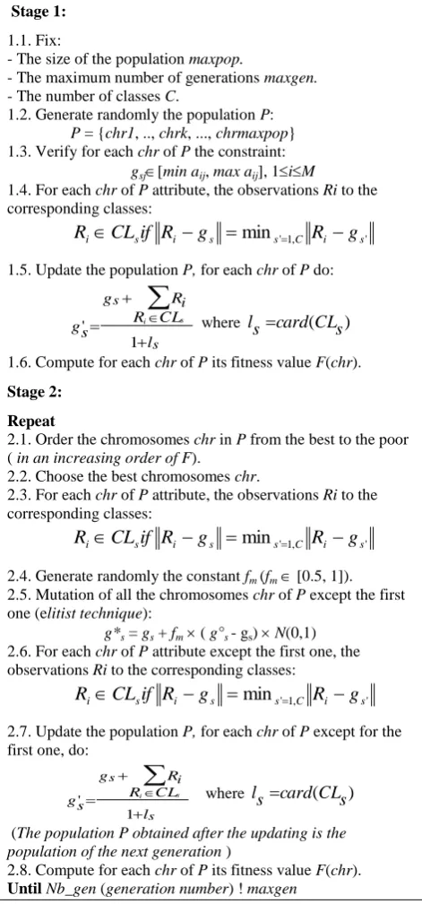
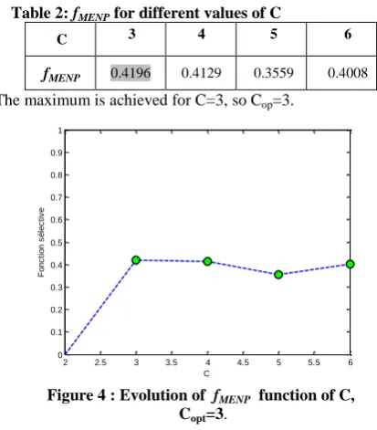
Table 2: fMENP for different values of C

C 3 4 5 6

fMENP 0.4196 0.4129 0.3559 0.4008

The maximum is achieved for C=3, so Cop=3.

Figure 4 : Evolution of fMENP function of C,

Copt=3.

One notices that the number of classes gotten by the algorithm of the entropy maximum coincides precisely with the real number of the classes.

SYNTH1 image segmentation with C=3

[image:4.595.338.505.315.446.2]

Figure 5 shows the results of segmentation by KM and EKM algorithms (three successive trials).

Figure 5 : Result of image segmentation

The EKM algorithm converges quickly in 2 generations as shown in figure 6.

[image:4.595.57.264.413.649.2]

Figure 6: Fitness value with respect to the generation. Synth1 image segmentation results are summarised in table 3.

Table 3: results of segmentation for Synth1 image

The results show that the EKM clearly detects the all objects of the image, background, big oval part, small oval part and lines. The KM was not able to detect the small oval part and lines.

The two algorithms were run several times and the EKM obtains each time the same result while the KM obtains different results. Wecan conclude that the EKM is the most stable; it outperforms the KM and obtains good results.

6.3. Blister pads image

In this phase of testing, an image of blister pads of size 79 * 81 which contains 10 stamps of longitudinal shape is taken, figure 7. The objective is to check whether there is any tablet in the pad lacking or damaged. The window that is considered is of size 3 * 3.

20 40 60 80 100 120 140 20

40 60 80 100 120

2 2.5 3 3.5 4 4.5 5 5.5 6

0 0.1 0.2 0.3 0.4 0.5 0.6 0.7 0.8 0.9 1

C

F

o

n

c

ti

o

n

s

é

le

c

ti

v

e

Originale EKM KM

0 5 10 15 20 25 30

0 0.5 1 1.5 2 2.5 3 3.5 4 4.5

5x 10 8

Class Region

description Level of gray

Number of pixels

1 background 255 6755 2 _{(included lines)}Big oval part 60 7339 3 Small oval part 0 3352

description EKM KM

Trial1 Trial2 Trial3 Trial1 Trial2 Trial3

background 6755 6755 6755 12410 6755 12410

Big oval part

(included lines) 7339 7339 7339 0 7339 0

Small oval

[image:4.595.311.535.495.579.2]

(5)

Figure 7: The original image

[image:5.595.322.514.74.297.2]

With the maximum entropy function the values shown in table 4 and figure 8 are gotten:

C 3 4 5 6

fMENP 0.2220 0.4129 0.3559 0.4008

Figure 8 : Evolution of fMENP function of C, Copt=4.

Pad image segmentation with C=4

The segmentation results in this case are shown in figure 9 for three different running of the KM and EKM algorithms. The result show that EKM clearly detects the damage accruing on one of the tablets for the three running while the KM fails to detect the defect for each.

Figure 9: Results of image segmentation

Table 5: number of pixels for any class Class

number Trial 1 Trial 2 Trial 3

EKM

CL1 CL2 CL3 CL4

92 1216 1317 3774

KM

CL1 CL2 CL3 CL4

984 1161 1184 3070

988 1161 1184 3066

984 1161 1184 3070

Figure 10 : Fitness value with respect to the generation.

Figure 10 shows the convergence of EKM algorithm, convergence is achieved very quickly, in three iterations, table 5 shows the results obtained by KM and EKM algorithms with details obtained on the classes for each running test. The EKM is more stable and has outperformed the KM algorithm.

6.4. Small disc image

In this phase of testing, an image of small disk of size 49 * 270 (figure 11) is taken. The objective is to detect the crack on the small disk. The window that isconsidered is of size 3 * 3.

Figure11: The original image

[image:5.595.57.249.210.407.2]

With the maximum entropy function the values shown in table 6 and figure 12 are gotten:

C 3 4 5 6

fMENP 0.6718 0.4652 1.1619 1.0328

Figure 12: Evolution of fMENP function of C, Copt=5.

2 2.5 3 3.5 4 4.5 5 5.5 6

0 0.1 0.2 0.3 0.4 0.5 0.6 0.7 0.8 0.9 1

C

F

o

n

c

ti

o

n

s

é

le

c

ti

v

e

EKM KM

0 5 10 15 20 25 30

0 1 2 3 4 5 6 7x 10

7

2 2.5 3 3.5 4 4.5 5 5.5 6

0 0.2 0.4 0.6 0.8 1 1.2

C

F

o

n

c

tio

n

s

é

le

c

tiv

[image:5.595.99.237.527.737.2] [image:5.595.319.508.557.739.2]

(6)

Small disk image segmentation with C=5

[image:6.595.105.231.132.307.2]

The segmentation results in this case are shown in figure 13 for three different running of the KM and EKM algorithms. The result show that EKM clearly detects the crack on the disk for the three running while the KM fails to detect the defect.

[image:6.595.62.258.339.623.2]

Figure 13 : Results of image segmentation

Table 7 : number of pixels for any class Class

number Trial 1 Trial 2 Trial 3

EKM

CL1 CL2 CL3 CL4 CL5

240 418 578 1320 1854

KM

CL1 CL2 CL3 CL4 CL5

327 400 880 998 1805

Figure 14 : Fitness value with respect to the generation.

Figure 14 shows the convergence of EKM algorithm, convergence is achieved very quickly, table 7 shows the results obtained by KM and EKM algorithms with details obtained on the classes for each running test. The EKM is more stable and has outperformed the KM algorithm.

7. CONCLUSION

Kmeans image segmentation shows some stability difficulties due to the initialisation problem. The evolutionary Kmeans image segmentation is proposed in order to get around this

difficulty. The proposed approach has been validated on synthetic and real images.

The experimental results obtained show the rapid convergence and the good performance of this approach. The instability problem has been eliminated.

The principle of maximum entropy is used to correctly estimate the optimal number of classes.

This approach may be used for problems of decision support in quality control.

8. REFERENCES

[1] Cocquerez T.P. et Phillip S. "Analyse d'images : Filtrage et segmentation". Editions MASSON, Paris, 1995.

[2] N.Vandenbroucke, L.Macaire, J.G. Postaire, Color image segmentation by pixel classification in an adapted hybrid color space. Application to soccer image analysis., Computer Vision and Image Understanding 90 (2), 190-216, 2003.

[3] Christophe Saint-Jean, Classification paramétrique robuste partiellement supervisée en reconnaissance des formes, Thèse de Doctorat, université de La Rochelle - UFR Sciences Laboratoire d’Informatique et d’Imagerie Industrielle 2001.

[4] L. Macaire, N. Vandenbroucke, J.G Postaire Segmentation d'images par classification spatio-colorimétrique des pixels. Traitement du signal vol 21 N spécial L'image numérique couleur 423-437, 2004.

[5] Nasri M. Contribution à la classification de données par Approches Evolutionnistes : Simulation et Application aux images de textures’’. Thèse de doctorat. Université Mohammed premier Oujda 2004.

[6] Nasri M, M. EL Hitmy, H. Ouariachi and M.Barboucha. Optimization of a fuzzy classification by evolutionary strategies. In proceedings of SPIE Conf., 6 th international conference on quality control by artificial vision, vol. 5132, pp. 220230, USA,. Repulished as an SME Technical Paper by The society of manufacturing, 2003.

[7] Hall, L. Q., Özyurt, I. B. et Bezdek, J. C. " Clustering with a genetically optimized approach ". IEEE Trans. on Evolutionary Computation, Vol.3, N°2, pp. 103-110, july 1999.

[8] H.Ouariachi, Classification non –Supervisée de données par les réseaux de neurones et par une approche évolutionniste : application à la segmentation d’images. Thèse de doctorat. Université Mohammed premier Oujda 2001.

[9] Presberger, T., Koch, M. “Comparison of evolutionary strategies and genetic algorithms for optimization of a fuzzy controller”. Proc. of EUFIT’95, Aachen, Germany, august 1995.

[10] Bezdek, J. C. "Cluster validity with fuzzy sets". J. Cybernetics, Vol.3, N°3, pp. 58-73, 1974.

[11] Karayiannis, N. B., Bezdek, J. C. et Hathaway, R. J. "Repairs to GLVQ : a new family of competitive learning schemes". IEEE Trans. on Neural Networks, Vol.7, N°5, pp. 1062-1071, 1996.

Originale EKM KM

0 5 10 15 20 25 30

0 2 4 6 8 10 12 14 16 18x 10

(7)

[12] A. EL Allaoui, M. Merzougui, M. Nasri, M. EL Hitmy and H. Ouariachi. Optimization of Unsupervised Classification by Evolutionary Strategies. IJCSNS International Journal of Computer Science and Network Security, ISSN: 1738-7906, Vol. 10 No. 6 pp. 325-332 June, 2010.

[13] M. Merzougui, A. EL Allaoui, M. Nasri, M. EL Hitmy and H. Ouariachi. Unsupervised classification using evolutionary strategies approach and the Xie and Beni criterion. IJAST International Journal of Advanced Science and Technology, ISSN: 2005-4238, Vol. 19, pp 43-58 June, 2010.

[14] Ammor.O, Raiss.N et Slaoui.K "Détermination du nombre optimal de classes présentant un fort degré de chevauchement " Revue Modulad N° 37, pp 31-42, 2007.

[15] G.Palubinskas, X. Descombes et F. Kruggel. " An unsupervised clustering method using the entropy minimization. " In ICPR, pp. 1816-1818, Australia Août 1998.