Constructive General Bounded Integral Control

http://dx.doi.org/10.4236/ica.2014.53017

Constructive General Bounded Integral

Control

Baishun Liu

Academy of Naval Submarine, Qingdao, China Email: [email protected]

Received 1 June 2014; revised 5 July 2014; accepted 15 July 2014

Copyright © 2014 by author and Scientific Research Publishing Inc.

This work is licensed under the Creative Commons Attribution International License (CC BY). http://creativecommons.org/licenses/by/4.0/

Abstract

This note proposes a systematic and more generic method to construct general bounded integral control. It is established by defining three new function sets and citing two function sets to con-struct three kinds of general bounded integral control actions and integrators, resorting to a uni-versal strategy to transform ordinary control into general integral control and adopting Lyapunov method to analyze the stability of the closed-loop system. A universal theorem to ensure regional-ly as well as semi-globalregional-ly asymptotic stability is provided in terms of some bounded information, and even does not need exact knowledge of Lyapunov function. Its one feature is that the indis-pensable element used to construct the general integrator can be taken as any integrable function, which satisfies Lipschitz condition and the self excited integral dynamic is asymptotically stable. Another feature is that the method to construct general bounded integral control action is ex-tended to a wider function set. Based on this method, the control engineers not only can choose the most appropriate control law in hand but also have more freedom to construct the bounded integral control actions and integrators, and then a high performance integral controller is more easily found. As a result, the generalization of the bounded integral control is achieved.

Keywords

General Integral Control, Nonlinear Control, Bounded Integral Control, General Nonlinear Integrator, Output Regulation

1. Introduction

The results, however, were local. The regional as well as semi-global results were proposed in [3], where the sliding mode manifold was used as the integrator, and then general integral control design was achieved by us-ing slidus-ing mode technique and linear system theory. In 2013, a class of nonlinear integrator, which was shaped by diffeomorphism, was proposed by [4], where feedback linearization technique was used to analyze the closed-loop system stability. General concave integral control was proposed in [5], where a class of concave function gain integrator is presented and the partial derivative of Lyapunov function is introduced into the inte-grator design. In consideration of the twinning of the concave and convex concepts, general convex integral control was proposed by [6], where the method to design the convex function gain integrator is presented and its highlight point is that the integral control action seems to be infinity but its factually is finite in time domain. Although general concave and convex integral control are all bounded integral control, one major limitation of them is that the indispensable element of the integrator is limited to the partial derivative of Lyapunov function, another is the function sets, which are used to design the general concave and convex integrator and integral control action, only were limited to two kinds of function sets. These two limitations become a serious obstruc-tion to design a high performance integral controller. In addiobstruc-tion, the generalizaobstruc-tion of the integrator and integral control action, which is achieved by defining two function sets, respectively, was proposed by [7], and its one drawback is that the integral control action could tend to infinity.

In consideration of the limitation of general concave and convex integral control, the aim of this paper is to propose a systematic and more generic method to construct general bounded integral control such that for a par-ticular application, the control engineers not only can choose the most appropriate control law in hand but also have more freedom to construct the bounded integral control action and integrator. The main contributions are as follows: 1) three new function sets are defined, respectively; 2) three kinds of method to construct general bounded integral control action and integrator are proposed; 3) the indispensable element used to construct the integrator is not confined to the partial derivative of Lyapunov function [5] [6] and function set [7], which is used to construct the integrator, and can be taken as any integrable function, which satisfies Lipschitz condition and the self excited integral dynamic is asymptotically stable; 4) the function sets used to construct the bounded integral control action have a wider range of choice than the corresponding function sets proposed by [5]-[7]; 5) a class of positive define bounded gain function is introduced into the integrator, which provides the designer with additional degrees of freedom to improve the control performance; 6) exact knowledge of Lyapunov func-tion is not necessary and it only needs to satisfy some bounded informafunc-tion; 7) by using Lyapunov method and LaSalle’s invariance principle, a universal theorem to ensure regionally as well as semi-globally asymptotic sta-bility is established. As a result, the generalization of the bounded integral control is achieved.

Throughout this paper, we use the notation λm

( )

A and λM

( )

A to indicate the smallest and largest

eigen-values, respectively, of a symmetric positive define bounded matrix A x

( )

, for any n

x∈R . The norm of vector

x is defined as x = x xT , and that of matrix A is defined as the corresponding induced norm

( )

T M

A = λ A A .

The remainder of the paper is organized as follows. Section 2 describes the system under consideration, as-sumption, definition and proof of Lemma. Section 3 addresses the method to construct general bounded integral control. Conclusions are presented in Section 4.

2. Problem Formulation

Consider the following nonlinear system,

(

)

(

)

(

)

, ,

,

x f x w g x w u

y h x w

 = +

  = 



(1)

where x∈Rn is the state, u∈Rmis the control input, y∈Rm is the controlled output, w∈Rl is a vector of unknown constant parameters and disturbances. The function f , g and h are continuous in

(

x w u, ,

)

on the whole control domain D_x×D_u×D_w⊂Rn×Rm×Rl. Let r∈D_r ⊂Rm be a vector of constant reference. Set ϑ ≡

(

r w,

)

∈Dϑ and Dϑ ≡Dr×Dw. We want to design a feedback control law u such that y t

( )

→r as

t→ ∞.

(

)

(

)

(

)

0 0 0

0

0 , ,

,

f x w g x w u

y r h x w

 = +

  = =

 (2)

so that x₀ is the desired equilibrium point and u₀ is the steady-state control that is needed to maintain equili-brium at x₀, where y=r.

No loss of generality, we state all definitions, theorems and assumptions for the case when the equilibrium point is at the origin of Rn, that is, x₀=0.

Assumption 2: No loss of generality, suppose that the function g x w

(

,

)

satisfies the following inequalities,

(

,

)

m 0 w, x

g x w >g > ∀ ∈w D ∀ ∈x D (3)

(

,

)

(

0,

)

gx w, x

g x w −g w ≤l x ∀ ∈w D ∀ ∈x D (4) where x

g

l is a positive constant.

Assumption 3: Suppose that there exists a control law u_x

( )

x such that x=0 is an exponentially stable equilibrium point of the system (5) and the inequality (6) hold,

(

,

)

(

0,

)

(

,

) ( )

x

x= f x w − f w +g x w u x (5)

(

,

)

(

0,

)

(

,

) ( )

x xf

f x w − f w +g x w u x ≤l x (6) and there exists a Lyapunov function V_x

( )

x such that the following inequlities,

( )

2 2

1 x 2

c x ≤V x ≤c x (7)

( )

4 x

V x

c x

x

∂

≤

∂ (8)

( ) ( ) ( ) ( ) ( )

(

)

2 3

, 0, ,

x

x

V x

f x w f w g x w u x c x

x

∂

− + ≤ −

∂ (9)

hold for all x∈Dx,ϑ∈Dϑ, where , ,1 2, 3 x

f

l c c c and c₄ are all positive constants.

For the purpose of this paper, it is convenient to introduce the following definitions and Lemmas. For the convenient comparison with the general concave and convex integral control, it is necessary to explain that the following Definition 1 and 2 was proposed by reference [5] [6], respectively.

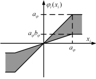
Definition 1: Fϕ

(

a b xϕ, ϕ,

)

with aϕ >0, 1≥bϕ >0 and x∈Rn denotes the set of all continuous

differen-tial increasing bounded functions [5] [8],

( )

( )

( )

( )

T

1 1 2 2 n n

x x x x

ϕ _{= }ϕ ϕ _ ϕ _

such that

( )

0 0

ϕ = ,

( )

i i i i

x ≥ϕ x ≥b x_ϕ , ∀ ∈xi R x:| i |<aϕ

( )

i i

a_ϕ ≥ϕ x ≥a b_{ϕ ϕ}, ∀ ∈xi R x:| i|≥aϕ

( )

(

)

1≥dϕi xi dxi>0 ∀ ∈xi R i=1, 2,,n .

where ⋅ stands for the absolute value.

Figure 1 depicts the region allowed for one component of functions belonging to function set F_ϕ. For in-stance, for all x∈R, hyperbolic tangent function, arc tangent function, Amosin function [8] and so on, all be-long to function set F_ϕ.

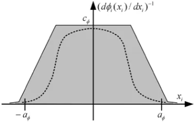
Definition 2: F a c x_φ

(

_φ, _φ,

)

with a_φ >0, 0c_φ > and x∈Rn, denotes the set of all continuous differential increasing functions [6],

( )

( )

( )

( )

T

1 1 2 2 n n

x x x x

[image:4.595.79.536.82.428.2]

Figure 1. The region allowed for one compo-nent of functions belonging to function set F_ϕ.

such that

( )

0 0 φ = ,

( )

(

)

1

(

)

0 dφi xi dxi cφ i 1, 2, ,n −

< < = _

and given any ε >0, there exists a positive constant a_φ such that

( )

(

)

1

dφ_i x_i dx_i − <ε ∀ ∈x_i R x: _i >a_φ. where ⋅ stands for the absolute value.

Figure 2describes an example curve and the region allowed for the derivative reciprocal of one component of functions belonging to function set F_φ. For instance, for all x∈R, the functions,

(

x+x5

)

3.0, sinh

( )

x ,

3

x+x and so on, all belong to function set F_φ.

Definition 3: F_ψ

(

a b_ψ, _ψ,x

)

with a_ψ >0, 0b_ψ > , and x∈Rn denotes the set of all continuous differential increasing functions,

( )

( )

( )

( )

T

1 1 2 2 n n

x x x x

ψ _{= }ψ ψ  ψ _

such that

( )

0 0

ψ = ,

( )

:

i xi bψ xi R xi aψ

ψ ≥ ∀ ∈ >

( )

(

)

dψi xi dxi>0 ∀ ∈xi R i=1, 2,,n .

Figure 3 depicts the example curves for one component of functions belonging to function set F_ψ . For in-stance, for all x∈R, the functions, _arcsinh

( )

_{x , tanh}

( )

_{x ,ax+bx}3 _{with a>0 and b}>_0,

( )

sinh x , and so on, all belong to function set F_ψ .

Definition 4: F_β

(

a c_β, _β,x

)

with a_β >0, 0c_β > and n

x∈R denotes the set of all continuous positive de-fine bounded functions,

( )

( )

( )

( )

T

1 1 2 2 n n

x x x x

β _{= }β β _ β _

such that

( )

0

(

1, 2, ,

)

i i i

c_β ≥β x > ∀ ∈x R i=  n , and given any ε >0, there exists a_β such that

( )

:

(

1, 2, ,

)

i xi xi R xi aβ i n

β <ε ∀ ∈ > = _ .

[image:4.595.213.383.85.224.2]

[image:5.595.194.402.82.617.2]

Figure 2. Example curve and the region allowed for the derivative reciprocal of one component of functions belonging to function set Fφ.

Figure 3. Example curves of functions belonging to function set Fψ.

Figure 4. Example curves and the region allowed for one component of functions belonging to function set

Fβ.

function set F_β. For instance, for all x∈R, the functions,

(

_{1 9}+ _x2

)

_cosh2

(

_x+_3x3

)

_{,1 cosh}2

( )

_{x ,1 1}

(

+_x2

)

_,

and so on, all belong to function set F_β.

Definition 5: F x_v

( )

with n x

x∈D ⊂R denotes the set of all integrable functions,

( )

( )

( )

( )

T

1 2 n

v x = _v x v x  v x _

[image:5.595.198.398.86.214.2] [image:5.595.198.397.263.436.2]

( )

x v

v x ≤l x ,

0

x= is an asymptotically stable equilibrium point of the self excited integral dynamic

( )

x= −v x for all x∈D_x.

where l_vx is a positive constant. For instance, for all x∈R, the functions, 3 3

( )

( )

, , , tanh , sinh

x x x+x x x

and so on, all belong to function set F_v.

Lemma 1: Let µ

( )

y ∈F_β or µ

( )

y =

(

dφ

( )

y dy

)

−1 with y∈R or φ

( )

y ∈F_φ, and then the function [6],

( )

(

( )

)

[

)

0

d 0,

t

y t =

∫

µ y τ τ ∀ ∈t ∞

is a positive define bounded increasing function, that is, 0<y t

( )

≤c∞ for all t∈

[

0,∞

)

, where c∞ is the

lim-it of y t

( )

as t→ ∞. Its proof consults the reference [6].

Lemma 2: Let µ

( )

z ∈Fβ or

( )

(

( )

)

1

d d

z z z

µ = φ − with z∈R, φ

( )

z ∈Fφ and v x

( )

∈Fv, and then the

function,

( )

(

( )

)

(

( )

)

[

)

0

d 0,

t

z t =

∫

µ z τ v x τ τ ∀ ∈t ∞

is bounded, that is, z t

( )

≤κ_∞ for all x∈D_x and t∈

[

0,∞

)

, where κ_∞ is a positive constant.

Proof: by definition of z t

( )

and Definition 5, we have,

( )

(

( )

)

(

( )

)

( )

(

( )

)

0 0

d max d

x

t t

x v x D

z t =

∫

µ z τ v x τ τ ≤l ∈ x

∫

µ z τ τ

Now, using Lemma 1, we obtain,

( )

max

( )

x x v x D

z t ≤c l_{∞ ∈} x =κ_∞.

Thus, z t

( )

is bounded, that is, z t

( )

≤κ_∞ for all x∈D_x and t∈

[

0,∞

)

.

Discussion 1: Comparing the two function sets F_ϕ and F_φ proposed by [5] [6] with the function set F_ψ , it is no hard to see that although they all claim that the function is continuous differential increasing function, the main differences are as follows: the limiting conditions of the function set F_ψ is less than the function sets F_φ

and F_ϕ. Thus, the function set F_ψ can completely includes the any functions belonging to the two function sets F_ϕ and F_φ.

Discussion 2: Comparing the function set [7], which was used to generalize the integral control action, with the function set F_ψ, the differences are the limiting condition about their derivatives, that is, the former de-mands cψ >dψi

( )

xi dxi>0 (cψ >0,∀ ∈xi R and i=1, 2,,n). However, the latter only requires

( )

dψi xi dxi>0. Thus, the function set Fψ not only can completely include the any functions belonging to the

function set proposed by [7] but also the functions belonging to the function set Fψ have a wider range of

choice than the one proposed by [7].

Discussion 3: Comparing the function set [7], which was used to generalize the integrator, with the function set F_v, the differences are that: the former is defined by resorting to Mean Value Theorem, therefore, it requires that the function is differential. However, the latter is defined by designing a self excited integral dynamic, and only demands its origin is asymptotically stable, and then differentiability condition is removed. Thus, it is not hard to see that the function set F_v not only can completely include the any functions belonging to the function set proposed by [7] but also the functions belonging to the function set F_v have a wider range of choice than the one proposed by [7].

Discussion 4: It is obvious that the bound of function, z t

( )

, which is obtained by Lemma 2, is too conserva-tive and even is not of interest. The situation, however, is not as bad as it might seem. As shown by Figure 2

andFigure 3, we can use aβ or aφ as its approximate value in practice, corresponding to ε small enough.

3. Constructive Method

( )

( )

( )

(

)

1

( ) ( )

d d

x

u u x K

v x

σ σ

σ σ σ − µ σ

 = − Φ

 

= Φ

 (10)

where

( )

x

u x is an ordinary control law;

K_σ is a positive define diagonal matrix;

( )

( )

( )

( )

T

1 1 2 2 m m

σ  σ σ σ 

Φ = Φ_ Φ _ Φ _ is a continuous differential increasing function with Φ

( )

0 =0;

( )

( )

( )

( )

T

1 1 2 2 m m

µ σ _{= }µ σ µ σ _ µ σ _ is a positive constant vector or positive define vector function;

( )

v x belongs to function set F_v;

( )

(

)

1

( ) ( )

d d 1, 2, ,

i i i i i i v xi i m

σ = Φ σ σ − µ σ =  .

Thus, substituting (10) into (1), obtain,

(

)

(

) ( )

(

)

( )

( )

,

( ) ( )

, x ,

x f x w g x w u x g x w K

v x

σ σ

σ µ σ

 = + − Φ



Φ =





 (11)

By Assumption 1 and choosing K_σ to be nonsingular and large enough, and then set x=0 and x=0 of (11), obtain,

(

0,

)

( )

0

(

0,

)

g w K_σΦ σ = f w (12) Therefore, we ensure that there is a unique solution, σ₀, and then

(

0,σ₀

)

is a unique equilibrium point of the closed-loop system (11) in the control domain of interest. At the equilibrium point, y=r, irrespective of the value of w.

Now, the design task is to provide methods to construct the bounded integral control action and integrator in the control law (10) such that K_σΦ

( )

σ is bounded and

(

0,σ₀

)

is an asymptotically stable equilibrium point of the closed-loop system (11) in the control domain of interest. To achieve this objective, the methods can be summarized as follows:

Method 1: If we choose Φ

( )

σ ∈F_ϕ, and then by definition of F_ϕ, it is easy to know that the integral con-trol action is bounded for all m

R

σ ∈ . Thus, µ σ

( )

can be taken as any positive define bounded vector func-tion or positive constant vector, that is, 0<µ σi

( )

i ≤cβ with σ ∈i R and i=1, 2,,m. Consequently, we

have,

( )

σ c_σ m

(

c_σ a_ϕ

)

Φ ≤ = , and

( )

(

dΦ_i σ_i dσ µ σ_i

)

_i

( )

_i ≤c_β =c_Φ

(

c_Φ >0

)

.

As a result, the generalization of the general concave integral control is achieved.

Method 2: If we choose Φ

( )

σ ∈F_φ, and then design µ σ

( )

such that

( )

(

)

1

( )

dΦ_i σ_i dσ_i − µ σ_{i i} ∈F_β,

( )

(

dΦ_i σ_i dσ µ σ_i

)

_i

( )

_i ≤c_Φ

(

c_Φ >0

)

, and

( )

i i Fβ

µ σ ∈

hold for all σ ∈_i R and i=1, 2,,m. Thus, by Lemma 1 and 2, it is easy to know that this kind of integral control action is bounded in time domain, that is,

( )

σ c_σ m

Φ ≤

where

( )

(

)

max i

x i m i

( )

(

)

( )

max max

x x

x

x x D v x lv x D x

γ = _∈ ≤ _∈ ,

( )

(

)

( )

(

)

1

(

( )

)

0

lim t d d d

i

t i i i i i

c∞ = →∞

∫

Φ σ τ σ τ − µ σ τ τ, and

1, 2, ,

i=  m.

As a result, the generalization of the general convex integral control is achieved.

Method 3: If we choose Φ

( )

σ ∈F_ψ, constructive general bounded integral control can be divided into two cases: 1) if Φ

( )

σ is bounded, and then µ σ

( )

can be taken as any positive define bounded vector function or positive constant vector. The condition for Φ

( )

σ is the same as Method 1; 2) if Φ

( )

σ is unbounded for all

m

R

σ ∈ , and then µ σ

( )

needs to be designed like Method 2. The condition for Φ

( )

σ is the same as Method 2. It is obvious that this is a more generic method to construct general bounded integral control because the function set used to construct the bounded integral control action has a wider range of choice than the corres-ponding function sets proposed by [5]-[7]. Moreover, it is worth noting that µ σ

( )

can be designed like Me-thod 2 when Φ

( )

σ is bounded.

In addition, it is convenient to introduce the variable, aΦ, which is equal to aϕ, aφ and aψ, respectively,

corresponding to the above three kinds of choices of the function Φ

( )

σ .

Based on the control law u_x

( )

x and three kinds of integral control actions and integrators above, the fol-lowing theorem can be established.

Theorem 1: Under Assumptions 1 - 3, if there exists a positive define diagonal matrix K_σ such that the fol-lowing inequality,

( )

(

)

(

0,

)

m g Km σ a f w

λ Φ Φ ≥ (13) and the inequality (20) hold, and then

(

0,σ₀

)

is an exponentially stable equilibrium point of the closed-loop system (11). Moreover, if all assumptions hold globally, and then it is globally exponentially stable.

Proof: To carry out the stability analysis, we consider the following Lyapunov function candidate,

( )

( )

(

, 0

)

( )

T

x z

V xΦ σ − Φ σ =V x +z P z (14) where 12 21 x z P P

P P_σ

 

=  

 

P ,

( )

( )

0

x z

σ σ

 

= _{Φ − Φ} 

 ,

z

P is a positive define

(

n+m

) (

× +n m

)

matrix;

x

P is a n n× matrix; P_σ is a m×m matrix;

12

P is a m n× matrix, _{12 21}T

P =P , P g K₁₂ m σ >0.

Obviously, Lyapunov function candidate (14) is positive define. Therefore, our task is to show that its time derivative along the trajectories of the closed-loop system (11) is negative define, which is given by,

( )

( )

(

)

( )

( )

_{( )}

_{( )}

( )

(

( )

( )

)

(

( )

( )

)

( )

0 12 21 , T T

x z z

x T T T T

x x

T T

V x V x z P z z P z

V x

x x P x x P x x P P x

x P P x σ σ σ σ σ σ

σ σ σ σ σ σ

Φ − Φ = + +

∂

= + + + Φ + Φ

∂

+ Φ Φ − Φ + Φ − Φ Φ

+

  _{ }

 

  

 

 12

(

( )

( )

0

)

(

( )

( )

0

)

21

T T

P Φ σ − Φ σ + Φ σ − Φ σ P x

(15)

Substituting (12) into (11), we obtain,

(

)

(

) ( ) (

)

( )

(

)

(

)

(

) ( )

(

) (

)

(

)

( )

(

)

(

( )

( )

0

)

, , ,

, 0, ,

, 0,

0,

x

x

x f x w g x w u x g x w K

f x w f w g x w u x

g x w g w K

g w K

σ σ σ σ σ σ σ

= + − Φ

= − +

− − Φ

− Φ − Φ



Now, by the above three kinds of choices of the function Φ

( )

σ , we have,

( )

σ

(

d

( )

σ dσ µ σ

)

( ) ( )

v x c l_Φvx x

Φ = Φ ≤ (17)

Substituting (16) into (15), and using (3), (4), (6), (8), (9), (17) and Φ

( )

σ ≤c_σ m, we obtain,

( )

( )

(

)

( )

( )

( )

( )

( )

0 2 0 2 0 , T T

x z z

x

x x

V x V x z P z z P z

x σ x

σ σ

σ σ

ρ ρ σ σ

ρ σ σ

Φ − Φ = + +

≤ − + Φ − Φ

− Φ − Φ

  _{ }

(18)

where

(

)

(

)

3 12 21

4

2

2 ,

x x x

x f x v

x

x g

c l P c l P P

c P c lσ m Kσ

ρ = − − _Φ +

− +

(

)

(

)

(

)

(

)

4

12 21

2 0, 2

,

x

x x v

x x

f g

c P g w K c l P

l c l m K P P

σ

σ σ

σ σ

ρ = + + Φ

+ + + and

(

)

(

12

)

(

21

)

T

m g Km P m P g Km

σ

σ σ σ

ρ =λ +λ .

and then inequality (18) can be rewritten as,

( )

( )

(

, 0

)

T

V x Φ σ − Φ σ ≤ −η ηQ (19) where

( )

( )

0 x

σ

σ

 

= _{Φ − Φ} 

 

 

η , 0.5

0.5 x x x x σ σ σ σ ρ ρ ρ ρ  −  = ₋    Q .

The right-hand side of the inequality (19) is a quadratic form, which is negative define when

0.25 0

x

x x x

σ σ σ

σ

ρ ρ − ρ ρ > (20) Using the fact that Lyapunov function (14) is a positive define function and its time derivative is a negative define function if the inequalities (13) and (20) hold, we conclude that the closed-loop system (11) is stable. In fact, V=0 means x=0 and σ σ= ₀. By invoking LaSalle’s invariance principle [9], it is easy to know that the closed-loop system (11) is asymptotically stable.

Discussion 5: Compared to general convex and concave integral control [5] [6], it is easy to see that this pa-per is not a simple extension of them but proposes a systematic and more generic method to construct general bounded integral control. The main progresses are as follows: 1) the indispensable element v x

( )

used to con-struct the integrator can be taken any functions belonging to function set F_v and is not confined to the partial derivative of Lyapunov function ∂V_x

( )

x ∂x, which is used to construct the integrator in [5] [6]; 2) a positive define bounded gain function µ σ

( )

is introduced into the integrator, which can be used to improve the integral control performance; 3) a class of new function set F_β is defined, and then the method to construct general bounded integral control action and integrator is extended to a wider function set F_ψ . As a result, this is a fire new and more generic method to construct general bounded integral control action and integrator; 4) we need not exact knowledge of Lyapunov function V_x

( )

x and only need it satisfy some bounded information. Moreover, if the partial derivative of Lyapunov function is attached into the function v x

( )

, the stability condi-tions can be relaxed. All these mean that the control engineers have more freedom to design the integrator and bounded integral control action, and then a high performance integral controller is more easily found.

devote its mind to counteract the unknown constant uncertainties and filter out the other action, and then actua-tor saturation is easy to be removed in practice; 3) a positive define bounded gain function µ σ

( )

is introduced into the integrator, which provides the designer with additional degrees of freedom to improve the integral con-trol performance; 4) as mentioned at Discussion 2 and 3, the function sets F_v and F_ψ used to construct the integrator and integral control action, respectively, all have a wider range of choice than the corresponding func-tion sets proposed by [7].

Remark 1: From the statement above, It is obvious that: First, five function sets for constructing general bounded integral control action is enumerated; Second, three general methods to construct the bounded integral control action are proposed; Final, a universal theorem to ensure regionally as well as semi-globally asymptotic stability is established. Under the domination of this theorem, all of them synthesize a systematic and more ge-neric method to construct general bounded integral control together. Consequently, for a particular application, the control engineers not only can choose the most appropriate control law in hand but also have more freedom to design the bounded integral control action and integrator, and then a high performance integral controller is more easily found.

4. Conclusion

This paper is not a simple extension of general convex and concave integral control but proposes a systematic and more generic method to construct general bounded integral control. The main contributions are as follows: 1) three new function sets are defined, respectively; 2) three kinds of method to construct general bounded integral control action and integrator are proposed; 3) the indispensable element used to construct the integrator is not confined to the partial derivative of Lyapunov function [5] [6] and function set [7], which is used to construct the integrator, and can be taken as any integrable function, which satisfies Lipschitz condition and the self ex-cited integral dynamic is asymptotically stable; 4) the function sets used to construct the bounded integral con-trol action has a wider range of choice than the corresponding function sets proposed by [5]-[7]; 5) a class of positive define bounded gain function is introduced into the integrator, which provides the designer with addi-tional degrees of freedom to improve the control performance; 6) exact knowledge of Lyapunov function is not necessary and it only needs to satisfy some bounded information; 7) by using Lyapunov method and LaSalle’s invariance principle, a universal theorem to ensure regionally as well as semi-globally asymptotic stability is es-tablished. As a result, the generalization of the bounded integral control is achieved.

References

[1] Liu, B.S. and Tian, B.L. (2009) General Integral Control. Proceedings of the International Conference on Advanced Computer Control, Singapore, 22-24 January 2009, 136-143. http://dx.doi.org/10.1109/ICACC.2009.30

[2] Liu, B.S. and Tian, B.L. (2012) General Integral Control Design Based on Linear System Theory. Proceedings of the

3rd International Conference on Mechanic Automation and Control Engineering, 5, 3174-3177.

[3] Liu, B.S. and Tian, B.L. (2012) General Integral Control Design Based on Sliding Mode Technique. Proceedings of the

3rd International Conference on Mechanic Automation and Control Engineering, 5, 3178-3181.

[4] Liu, B.S., Li, J.H. and Luo, X.Q. (2014) General Integral Control Design via Feedback Linearization. Intelligent Con-trol and Automation, 5, 19-23. http://dx.doi.org/10.4236/ica.2014.51003

[5] Liu, B.S., Luo, X.Q. and Li, J.H. (2013) General Concave Integral Control. Intelligent Control and Automation, 4, 356- 361. http://dx.doi.org/10.4236/ica.2013.44042

[6] Liu, B.S., Luo, X.Q. and Li, J.H. (accepted) General Convex Integral Control. International Journal of Automation and Computing.

[7] Liu, B.S. (submitted) On the Generalization of Integrator and Integral Control Action. International Journal of Modern Nonlinear Theory and Application.

[8] Kelly, R. (1998) Global Positioning of Robotic Manipulators via PD Control plus a Class of Nonlinear Integral Actions.

IEEE Transactions on Automatic Control, 43, 934-938. http://dx.doi.org/10.1109/9.701091

currently publishing more than 200 open access, online, peer-reviewed journals covering a wide range of academic disciplines. SCIRP serves the worldwide academic communities and contributes to the progress and application of science with its publication.

Other selected journals from SCIRP are listed as below. Submit your manuscript to us via either