Cost Evaluation In Seismic Analysis And Aseismic
Design Of Rc Framed Structure
R.Regupathi1, R.Prakash2
1
R. Regupathi, Department of Civil Engineering, Government College of Engineering, Bodi-625 582, Tamilnadu, India 2
Department of Civil Engineering, A.C. College of Engineering and Technology,Karaikudi-630 003, Tamilnadu, India
Abstract: Determination of design lateral forces is the primary requirement of seismic analysis and design of a structure. The aim of this work is to analyse and design multi-storeyed RC frames for earthquake forces for different seismic zones in India. The lateral forces due to Earthquake were evaluated as per IS1893 (Part1):2002, by Response Spectrum method and Seismic co-efficient method by programs developed in MATLAB. Also increase in cost of construction of earthquake resistant frames is compared with that of the conventional design by analysing a twelve storey building with Ordinary Moment Resisting Frame (OMRF) and Special Moment Resisting Frame (SMRF). Lateral forces on the SMRF and OMRF due to earthquake in all zones of India were obtained by using the MATLAB program for Seismic co-efficient method and the analysis and design for critical load combinations were carried out in STAAD. Pro. It is found that there is only a marginal increase in cost of 8% to 40% for both the type of construction in zone II to IV from the conventional frame. While increase in cost of construction in zone V is 50 % and 53% respectively for SMRF and OMRF. Hence it is advisable to design multi-storeyed RC frames considering seismic forces in all earthquake zones of India and also as a Special Moment Resisting Frame for the safety of men and material
Keywords: Response Spectrum, Seismic Coefficient, Seismic Zone, Dynamic Response, Time History
I. INTRODUCTION
The recent earthquake that have occurred in Indian Sub-continent have given a fillip to the study of earthquake engineering in the last one or two decades. A few IS codes have come up subsequently suggesting measures to improve the earthquake resistance of different category of structures. Latest codes on earthquake resistant design of structures give guidelines for reduction of seismic forces through provision of special ductility requirements. The magnitude of the forces induced in the structure due to a given ground acceleration will depend on the damping and ductility. By enhancing ductility and energy dissipation capacity in the structure, the induced seismic forces can be reduced, a more economical structure obtained and the probability of collapse is reduced. It is not always possible to design reinforced concrete structures to resist short duration extreme loads which are reversible after the event, purely from economic considerations. Seismic loading is one example of such loading. Considerable economy can be achieved by allowing inelastic deformations in the structure and its components. Within certain limits of damage, it may be even possible to repair and reuse the structure. For extremely high loads, the design philosophy can be that the structure undergoes enormous deformation, absorbs energy, but does not fail. This design approach is called ductility based design approach. The provisions given for seismic loading in IS1893(Part1):2002, “Criteria for Earthquake Resistant Design of Structures” have included certain ductility demand on the structure. IS13920 -1993 on “Ductile detailing of reinforced concrete structures subjected to seismic forces” are mandatory for all the structures located in seismic zone III.
II. RESPONSEOFSTRUCTURESTOEARTHQUAKE
Structures on earth are subjected to two types of load: Static and Dynamic. Static loads are constant with time while dynamic loads are varying. These loads can be further divided as shown in Fig 2.1.In general, majority of the structures are designed assuming that all applied loads are static. The effect of dynamic load is not considered because the structure is subjected to dynamic loads rarely; more so, its consideration in analysis makes the solution more complicated and time consuming. This feature of neglecting the dynamic forces may sometimes become the cause of disaster, particularly, in case of earthquake. The recent example of this category is Bhuj earthquake of January26,2001. Nowadays there is a growing interest in the process of designing Civil Engineering structures capable of withstanding dynamic loads, particularly, earthquake induced load.
LOADS
STATIC DYNAMIC
PRESCIBED RANDOM
(Deterministic) (Probabilistic)
PERIODIC NON-PERIODIC
HARMONIC NON-HARMONIC TRANSIENT IMPULSIVE
Machine Human motion, Earthquake, wind, Impact blast, operation machine operation. water waves, traffic. explosion
FIG: 2.1 -Various types of static-dynamic loads
A. Static And Dynamic Equilibrium
The basic equation of static equilibrium under displacement method of analysis is given by F (ext) = ky --- (1)
where F (ext) is the external applied static force, k is the stiffness resistance and y is the resulting displacement. The restoring force (ky) resists the applied force, F (ext). The restoring force is the function of the yield condition in the structure, which in turn is a function of time. The stiffness parameter k is a potential source of discrepancy, and is affected by the quality of material, age, cracking, support condition etc. The forcing function F is often difficult to estimate, particularly in case of earthquake.Now, if the applied static force changes to dynamic force or time varying force the equation of static equilibrium becomes one of the dynamic equilibrium and has the form
F (t) = m (d2y/dt2) + c (dy/dt) + ky --- (2)
If we do a direct comparison of Equations 1 and 2, we shall find the two additional forces that resist the applied forces with the restoring forces. These additional forces are called inertia force [m (d2y/dt2)] and damping force [c (dy/dt)] resulting from the induced acceleration and velocities in the structure. The appearance of inertia and damping forces in the structure during a dynamic loading is the most characteristic distinction between static loading and dynamic loading effects.
2) Dampin: The energy produced in the structure by the ground motion is dissipated through internal friction within the structural and non-structural members. This dissipation of energy is called damping. The structures always possess some intrinsic damping, which diminishes with time once the seismic excitation stops. These dissipative or damping forces are represented by viscous damping forces, which are proportional to the velocity induced in the structure. The constant of proportionality is called as linear viscous damping. The value of damping depends on its components, component connections, materials etc. The amount of damping in a structural system cannot be analytically ascertained, it must be determined experimentally. In practice this damping effect is expressed as percentage of critical damping which is the greatest damping value that allows vibratory movement to develop. Experience has made it possible to estimate the degree of damping in various types of structures, and the value of damping for some common types of structures are reinforced concrete 5-10%.metal frame 1-5%, masonry 8-15%, wood structures 15-20% .
3) Ductility And Fundamental Period The restoring force in the structures is proportional to the deformation induced in the structure during seismic excitation. The constant of proportionality is referred as stiffness of the structure. Stiffness greatly affects the structure’s uptake of earthquake-generated forces. On the basis of stiffness, the structure may be classified as brittle or ductile. Brittle structure having grater stiffness proves to be less durable during earthquake, while ductile structure performs well in earthquakes. This behaviour of structure evokes an additional desirable characteristic called ductility. Ductility is the ability of the structure to undergo distortion or deformation without damage or failure. Inertia forces are most significant which depend upon the characteristics of the ground motion and structural characteristics of structure. The basic characteristic of the structure and ground is its fundamental or natural period. The fundamental periods of structures may range from 0.05 second foe well anchored piece of equipments, 0.1 second for a one-storey frame,0.5 second for low structure up to about 4 stories and between 1-2 seconds for tall building of 10-20 stories. Natural periods of ground are usually in the range of 0.5 to 2 seconds, so it is possible for the building and the ground to have same fundamental period and therefore there is a high probability for the structure to approach a state of partial resonance (quasi-resonance). Hence in developing a design strategy for a building, it is desirable to estimate the fundamental periods both of the structure and of the site so that a comparison can be made to see the existence of the probability of quasi-resonance.
III. SEISMIC ANALYSIS OF STEEL FRAMES
Once the structural model is selected, it is possible to perform analysis to determine the seismically induced forces in the structures. There are different methods of analysis which provide different degrees of accuracy. The analysis process can be categorized on the basis of three factors: the type of externally applied loads, the behaviour of structure/structural materials, and the type of structural model selected. Based on the type of external action and behaviour of the structure, the analysis can be further classified as linear static analysis, linear dynamic analysis, non-linear static analysis or non-linear dynamic analysis.
A. Linear Static And Dynamic Analysis
his method is mainly suitable for regular buildings which respond primarily within the elastic range. Equivalent static load procedure or seismic coefficient method is specified in most of the design codes. A set of static loads are calculated based on the fundamental period of the structure and the seismic conditions at site (zone, importance factor, soil type). The loads are distributed along the height of the building in a manner consistent with the first mode shape. Higher mode effects are approximated by additional fraction of load applied at the roof level in many of the seismic codes. This analysis is normally performed either by manual calculations or using any analysis software. Linear dynamic analysis can be performed in two ways either by mode superposition method or response spectrum method and elastic time history method. This analysis will produce the effect of the higher modes of vibration and the actual distribution of forces in the elastic range in a better way. They represent an improvement over linear static analysis. The significant difference between linear static and dynamic analysis is the level of force and their distribution along the height of the structure.
B. Non - Linear Static And Dynamic Analysis
Non-linear static analysis is an improvement over the linear static or dynamic analysis in the sense that it allows the inelastic behaviour of the structure. The methods still assume a set of static incremental lateral load over the height of structure. The method is relatively simple to be implemented, and provides information on the strength, deformation and ductility of the structure and the distribution of demands. This permits to identify critical members likely to reach limit states during earthquake, for which attention should be given during the design and detailing process. But this method contains many limited assumptions, which neglect the variation of loading patterns, the influence of higher modes, and the effect of resonance. This method, under the name push over analysis has acquired a great deal of popularity nowadays and in spite of these deficiencies this method provides reasonable estimation of the global deformation capacity, especially for structures which primarily respond according to first mode. A non-linear dynamic analysis or inelastic time history analysis is the only method to describe the actual behaviour of the structure during an earthquake. The method is base on the direct numerical integration of the motion differential equations by considering the elasto-plastic deformation of the structural element. This method captures the effect of amplification due to resonance, the variation of displacements at diverse levels of a frame, an increase of motion duration and a tendency of regularization of movements as far as the level increases from bottom to top.
C. Code-Based Procedure For Seismic Analysis
Main features of seismic method of analysis base on Indian Standard 1893 (Part 1):2002 are described as follows:
1) Equivalent Lateral Force: Seismic analysis of most of the structures are still carried out on the basis of lateral(horizontal) force assumed to be equivalent to the actual (dynamic) loading. The base shear which is the total horizontal force on the structure is calculated on the basis of structure mass and fundamental period of vibration and corresponding mode shape. The base shear is distributed along the height of structure in terms of lateral forces according to Code formula. This method is usually conservative for low to medium height buildings with regular configuration.
2) Response Spectrum Analysis: This method is applicable for those structures where the modes other than the fundamental one significantly affect the response of the structure. In this method the response of Multi-Degree-of-Freedom(MDOF) system is expressed as the superposition of modal response, each modal response being determined from the spectral analysis of single-degree-of-freedom(SDOF) system, which are then combined to compute the total response. Modal analysis leads to the response history of the structure to a specified ground motion; however, the method is usually used in conjunction with a response spectrum.
IV. MODAL ANALYSIS OF MULTI-STOREYED FRAMES
a number of independent displacement coordinates, and modeling of the system as a multi degree of freedom (MDOF) system. Free vibration of the structure is initiated by disturbing the structure from its equilibrium position by some initial displacements and/or by imparting some initial velocities
For an undamped free vibration of structures, the equation of motion is given by [M]{ü} + [K]{u}=0
The above equation represents N homogeneous differential equations that are coupled through the mass matrix, the stiffness matrix, or both matrices; N is the number of DOFs. An undamped structure would undergo simple harmonic motion without change of deflected shape, however, if free vibration is initiated by appropriate distributions of displacements in the various DOFs. n characteristic deflected shapes exist for n DOF. If this system is displaced in one of these shapes and released, it will vibrate in simple harmonic motion, maintaining the initial deflected shape. All the floors reach their extreme displacements at the same time and pass through the equilibrium position at the same time. Each characteristic deflected shape is called a natural mode of vibration of an MDF system. A natural period of vibration Tn of an MDF system is the time required for one cycle of the simple harmonic motion in one of these natural modes. The corresponding natural circular frequency of vibration is ωn and the natural cyclic frequency of vibration is fn, where
Tn=2Π/ωn fn=1/Tn
Assume solutions of form ui =ai (sinωt-α), where i=1, 2, 3 …n. ai is the amplitude of motion of ith coordinate and n is the no of degree of freedom.
[[K]-[M] ω2]{a}=0
which is the homogenous algebraic system of linear equations with n unknown displacements ai, and unknown parameters ω2. The formulation of above equation is an important mathematical problem known as eigen problem. In order to have a non trivial solution
| [K]-ω2 [m]|=0
In general, above equation results in a polynomial equation of degree ‘n’ in ω2this should be satisfied for n values of ω2. The above
equation is termed as the characteristic equation. This equation has n real and positive roots for ωn2 because m and k matrices are symmetric and positive definite. The positive definite property of k is assured for all structures supported in a way that prevents rigid body motion. The positive definite property of m is also assured because the lumped masses are non zero in all DOFs retained in the analysis. The roots of this characteristic equation are called eigen values and the positive square root of the eigen values are known as natural frequency of the MDOF system.
For each eigen value the resulting (synchronous) motion has a distinct shape known as natural mode shapes or normal mode shape or eigen vector. There might be a number of eigen vectors. The n eigen vector can be displayed into a single square matrix, each column of which is a natural mode:
Ф= Ф11 Ф12 ….. Ф1n Ф21 Ф22 …... Ф2n . . . . . . . . . Фn1 Фn2 Фnn
m1
m2
m3
k2
The matrix Ф is called the modal matrix for the eigen value problem. The n eigen values can be assembled into a diagonal matrix
Ω2, which is known as the spectral matrix of the eigen value problem. In order to obtain a unique solution, eigen vectors are normalized using certain normalization conditions. Such a normalization using mass matrix is known as mass renormalization and the resulting mode shape is known as mass orthonormal mode shape.
A. Vector iteration method:
In the process of obtaining the eigen vales and eigen vectors, vector iteration method is employed. This method involves the assumption of a trial eigen vector and performing repeated matrix manipulations to converge to the desired eigen vector. Among the iteration techniques simultaneous iteration method is employed in determining the eigen values and vectors. The steps are as follows: Initially a trial vector set {x1}nxm is assumed. By some procedure orthonormal vector {x} is extracted from {x1}nxm.
ie., {x}T[M]{x}=[I] Compute {R}nxm=[M]nxn{x}nxm
Solve for {x2} from [K]nxn{x2}nxm={R}nxm
Compute [λ]mxm={x}T[K]{x}.
[λ] is now an (mxm) matrix ,the diagonal elements of which are our current approximation to the eigen values.
The iterations are continued till [λ] converges fully. When converged,[λ] will be of the form
λ1 ≈0 λ2 . . ≈0 λn
and the corresponding {x} will have the eigen vectors.
In the extraction of {x} vector from {x1} the cholesky factorization is used. The cholesky factorization is used to find upper triangular matrix or the lower triangular matrix. This factorization is done by
[A]= [L] T [L]
READ fck,b,d,h,Bx,By
E=5000√fck
I=b*d3/12
k=12*E*I/h3
M=TW*103/9.81
K= (Bx+1)*(By+1)* (kxn+kxn+1)
X=[I]
for i=1;1<=50;1++
d=[X]T*[M]*[X]
C=chol(d)
V. RESPONSE SPECTRUM METHOD
Dynamic analysis is carried out either by modal analysis procedure or dynamic analysis procedure (Clause 7.8 of IS 1893 (Part 1):2002).Dynamic analysis is recommended to obtain the design seismic force, and its distribution levels along the height of the building and to the various lateral load resisting elements, for the following buildings:
Regular buildings – those greater than 40 m in height in zones IV and V, and those greater than 90 m in height in zone II, and a
y=[X]*[C]-1
r=[M*[y]
X=[K]-1*[r]
i
λ=[y]T*[K]*[y]
ωn=√l
f=ωn/2Π
T=1/F
PRINT K, M, λ, ωn, y, T
All Irregular buildings(Tables 4,5) and all framed buildings higher than 12 m in zones IV and V, those greater than 40 m in height in zones II and III. For irregular buildings, less than 40 m in height located in zones II and III, dynamic analysis, though not mandatory, shall be preferred.
The purpose of dynamic analysis is to obtain the design seismic forces, with its distribution to different levels along the height of the building and to various lateral load resisting elements similar to the seismic co-efficient method. The procedure of dynamic analysis described in Code is valid only for regular type of buildings, which are almost symmetrical in plan and elevation about the axis having uniform distribution of the lateral load resisting elements. It is assumed that all masses are lumped at the storey level and only sway displacement is permitted in each storey. The dynamic analysis procedure for regular type building is divided into several distinctive steps, which are as follows:
Using the eigen-values and eigen-vectors determined by the modal analysis for the multi storey shear frame, modal participation factors and effective masses for all the all the modes are calculated.
A. modal participation factor (pk)
Modal participation factor of mode k of vibration is the amount by which the mode k contributes to the overall vibration of the structure under horizontal and vertical earthquake ground motions.
B. MODAL MASS,
M
kModal mass of a structure subjected to horizontal or vertical, as the case may be, ground motion is a part of the total seismic mass of the structure that is effective in mode k of vibration.
where,
g - Acceleration due to gravity.
ik
- Mode shape co-efficient at floor i in mode k. Wi - Seismic weight at floor i.C. Modal Contributions For Various Modes
It is clear from the values of the participation factors and effective mass, their value decreases as mode number increases. The practical significance of this fact is that in general it is necessary to include all the modes in the calculation. Only a few significant modes need to be included in order to obtain reasonable results for practical problems. Therefore, the Clause 7.8.4.2 of IS1893 (Part 1):2002 states, that “The number of modes to be used in the analysis should be such that the sum of total modal masses of all modes considered is at least 90% of the total seismic mass and missing mass correction beyond 33 Hz are considered, modal combination shall be carried out only for modes upto 33 Hz”
Modal contribution of various oes, for mode i =
M
Mi
%
D. Design Lateral Force At Each Floor In Each Mode
The design lateral force Qik at floor i in mode k i is given by
21 2 1 ik N i i ik N i i k
W
g
W
M
22
Z
R
I
g
S
aQik = Ak
ikPk Wi whereAk - design horizontal acceleration spectrum value as per 6.4.2 using the natural period of vibration Tk of mode k. The design horizontal seismic co-efficient Ak for various modes are worked out using
Ah =
Design lateral force in each mode
Qi1 = (A1 P1
ikWi) =
1
1
1
1
1
1
1
1
...
...
1
21
1
1
1
11
1
1
W
n
P
A
W
n
P
A
W
P
A
W
P
A
kNSimilarly Qi2,Qi3,Qi4……Qin
E.Storey Shear Forces In Each Mode
The peak shear force Vik acting in storey i in mode k as per Clause 7.8.4.5 is given by
The storey shear force for the first mode is,
=
Vn
Vn
V
V
1
21
11
=
Qn
Qn
Qn
Qn
Qn
Q
Qn
Qn
Q
Q
1
1
1
21
1
21
11
F. Storey Shear Forces Due To All Modes Considered
The peak storey shear force (Vi) in storey i due to all modes considered is obtained by combining those due to each mode in accordance with modal combination. as The combinations are usually achieved by using statistical methods. The design values for the total base shear are obtained by combining the corresponding modal responses. In general these modal maximum values will not occur simultaneously. To overcome this difficulty, it is necessary to use an approximate method. An upper limit for the maximum response may be obtained by the Sum of the AB solute values (ABS) of the maximum modal contributions. This is very conservative method and is very seldom used except in some codes for say two or three modes for very short period structures. If the system does not have closely spaced modes, another estimate of the maximum response, which is widely accepted and which usually provides a reasonable estimate is the Square Root of the Sum of Squares (SRSS). Application of the SRSS method for combining modal responses generally provides an acceptable estimation of the total maximum response. However , when some of the modes are closely spaced i.e. the difference between two natural frequencies is within 10% of the smallest of two frequencies, the use of SRSS method may either grossly underestimate or overestimate the maximum response. A formulation known as the Complete Quadratic Combination (CQC), based on the theory of random vibration and is also considered as the extension of SRSS method. For an undamped structure CQC estimate is identical to SRSS method.
G. Maximum Absolute Reponses (Abs)
r c c
*where, the summation is for closely spaced modes only. The peak response quantity due to the closely spaced modes (
*
) is then combined with those of the remaining well separated modes by the SRSS method.H. Square Root Of The Sum Of Squares (Srss)
A more reasonable method of combing modal maxima for two-dimensional structural system exhibiting well-separated vibration
frequencies is the square root of the sum of squares (SRSS). The peak response quantity (
) due to all modes considered shall be obtained as 2 1)
(
r k k
Where, k
- The absolute value of a quantity in mode k.r - Number of modes being considered.
Using the above method the storey shears are as follows,
V1 = [(V11)2+(V12)2+………(V1(n-1))2+(V1n)2]1/2 kN V2 = [(V21)2+(V22)2+………(V2(n-1))2+(V2n)2]1/2 kN V3 = [(V31)2+(V32)2+………(V3(n-1))2+(V3n)2]1/2 kN …….
…….
Vn = [(Vn1)2+(Vn2)2+………(Vn(n-1))2+(Vnn)2]1/2 kN
I.Combined Quadratic Combination (Cqc)
For three dimensional structural systems exhibiting well-separated vibration frequencies, the peak response quantities shall be combined as per Complete Quadratic Combination (CQC) method.
j ij r i r j
i
1 1 Where,r - Number of modes being considered.
i
- Response quantity in mode i (including sign).
j
- Response quantity in mode j (including sign).
ij
- Cross modal co-efficient.
2 2 2 5 . 1 2
)
1
(
4
)
1
(
)
1
(
8
ij ij ij ij ij
Where,
- Modal damping ratio (in fraction)ij
- Frequency ratio
j
i .i
j
- Circular frequency in jth mode.Here the terms
i and
j represent the response of different modes of a certain storey level. Using matrix notation the storeyshears V1, V2, …..Vn are worked out respectively
J. Lateral Forces At Each Storey Due To All Modes
The design lateral forces Froof and Fi at roof and at ith floor are calculated as, Froof = Fi, and Fi = Vi + Vi+1
Fn = Vn kN …. F2 = F2 kN F1 = V1 kN
K. Flowchart To Response Spectrum Method
Start
Calculate modal partication Factor in both direction – [pkx] ,[pky]
Calculate modal mass in both Direction – [mkx], [mky]
Read Z , I, R
Calculate Sa/g using Tx , Ty in both direction
A
` A
Calculate seismic-co efficient Ahx, Ahy in both `` the direction
Ah = (Z/2)x(Sa/g)x(I/R)
Calculate design lateral force in each mode Qx, Qy in both the direction
Calculate storey shear force in each mode Vkx ,Vky in both direction.
Vk = Σ Q
Calculate storey shear forces considering all modes
Maximum Absolute Square root of sum of Combined Quadratic Response Squares Combination
Calculate MARx, Calculate SRx, Sry Calculate CCx, MARy in both the in both the direction CCy in both the direction direction
Calculate design lateral Calculate design lateral Calculate design lateral force at each storey force at each storey force at each storey considering all modes considering all modes considering all modes LFmx, LFmy LFsx, LFsy LFcx, LFcy
Print LFmx,LFmy,LFsx,LFsy,LFcx,LFcy
End
VI. SEISMIC CO-EFFICEINT METHOD
This is the simplest method of analysis and requires less computational effort because the forces depend on the code based fundamental period of structures with some empirical modifier. The design base shear shall be first computed as a whole, then be distributed along the height of the buildings based on simple formulas appropriate for buildings with regular distribution of mass and stiffness. The design lateral force obtained as each floor level shall then be distributed to individual lateral load resisting elements depending upon on floor diaphragm action. In case of rigid diaphragm (reinforced concrete monolithic slab-beam floors or those consisting of pre-fabricated/precast elements with topping reinforced screed can be taken as rigid diaphragm) action, the total shear in any horizontal plane shall be distributed to the various elements of lateral force resisting system on the basis of relative rigidity (Clause 7.7.2 of IS1893 (Part 1):2002). The following are the major steps for determining the forces by equivalent static procedures.
A. Determination Of Base Shear
The total design lateral force or design base shear along any principal direction shall be determined by the following expression, Clause 7.5 of IS1893 (Part 1):2002.
2
Z
R
I
g
S
a Ah - Design horizontal seismic co-efficient for a structure. W - Seismic weight of the buildingSeismic weight of a building is the sum of the seismic weight of all the floors. The seismic weight of each floor is its full dead load plus percentage of imposed load as given Table 8 of IS1893 (Part 1):2002 as per clause 7.3.1. Imposed load on roof level need not be considered. The basic reasons for considering the percentage of live load as specified in Table 8 is that only part of maximum live load will probably be existing at the time of earthquake.
Design Horizontal Seismic Coefficient (Ah) of a structure for each mode of vibration is determined by the equation given below: Ah = `
Provided that for any structure with T ≤ 0.1 s, the value of Ah will not be taken less than Z/2 whatever the value of I/R
where
Z = Zone factor I = Importance Factor
R = Response Reduction Factor
Sa/g = Average Response Acceleration Coefficient
B. Zone Factor (Z)
The country is classified into four seismic zones for the purpose of determining the seismic forces and is given in the code.
Zone Factor ( Z ) is given in Table 2 in IS1893 (Part 1):2002 as per clause 6.4.2 for the Maximum Considered Earthquake ( MCE ) and service life of the structure in a zone. In Eqn. the factor 2 in the denominator of Z is used to reduce the Maximum Considered Earthquake zone factor to the factor for Design Basis Earthquake ( DBE ). The maximum intensity is fixed in such a way that the lifeline/critical structures will remain functional and there is low probability of collapse for structures with the provisions provided in the code even with for an event of occurrence of earthquake with higher intensity
C. Importance Factor ( I )
Importance Factor ( I ) given in Table 6 in IS1893 (Part 1):2002 as per clause 6.4.2 is depending upon the functional use of the structure. This value is characterised by hazardous consequences of failure of the structure, post-earthquake functional needs historical value or economical importance
D. Response Reduction Factor ( R )
Response reduction factor (R) depends on the seismic damage performance of the structure for ductile or brittle deformation. However the ratio I/R shall not be greater than 1.0. The values of R for the buildings are given in Table 7 in IS1893 (Part 1):2002 as per Clause 6.4.2.
E. Average Response Acceleration Co-Efficient
The average responseacceleration coefficient, Sa/g is based on the
1) appropriate natural periods,
2) type of soil and
3) damping of the structure. where,
Bureau of Indian Standards IS 1893 - 2002 specifies some empirical expressions for finding the approximate fundamental natural period of vibration in R.C. frame Building.For a moment-resisting frame building without brick infill panels, the approximate fundamental natural period of vibration (Ta) in seconds may be estimated by the empirical expression
Ta = 0.075 h0.75 for RC frame building Ta = 0.085 h0.75 for steel frame building
Ta =
d
h
09
.
0
where,
h - Height of the building in meters. This excludes the basement storeys, where basement walls are connected with the ground floor deck or fitted between the building columns. But it includes the basement storeys, when they are not so connected.
d - Base dimension of the building at the plinth level, in meters, along the considered direction of the lateral force.
The values of spectral acceleration coefficient for different natural periods has be taken from Response spectrum. A response spectrum is defined as a curve which shows the peak response of a single degree freedom oscillator (having a certain damping) to a given input ground motion. It shows the variation between peak acceleration as a function of acceleration due to gravity (Sa/g) on the Y axis and the natural period (T) on the X axis.
Fig: 6.1 Response spectra for 5 percent damping
F. Distribution Of Design Lateral Force
The computed base shear is now distributed along the height of the building. The shear force, at any level, depends on the mass at that level. IS1893 (Part 1):2002 uses parabolic distribution of lateral force along the height of the building as per the following expression.
Qi= VB
n
j
j j
i i
h
W
h
W
1 2 2
Where,
Qi – design lateral force at floor i. Wi – Seismic weight of floor i.
hi – Height of floor i measured from base.
READ Bx,By,l,b,Ns,h,bc,dc, bl,dl,OWT,IWT,LL,FST,WCT
H=h*Ns C=bc*dc
BS=bl*dl dx =B*l dy=B*b START
READ SZ, i, r, s
if SZ=3
if SZ=4 if
SZ=2
if SZ=5
Z=0.10 Z=0.16 Z=0.24 Z=0.36
if i=1 if i=2
I=1.5 I=1.0
if r=1 If r=2
R=5.0 R=3.0
Ta=0.075*H0.75(without infill&R.C)
Ta=0.085*H0.75(without infill&steel)
Ta=0.09*H/√dx(or)dy(with infill)
Calculate Sa/g depending on soil type(s)
Ah= (Z/2)*(I/R)*(Sa/g)
Calculate Total load-TW& Base Shear -VB
a
a
V=W*h2/Σ (W*h2) Q=VB*V
PRINT VB,V, Q
VII. COMPARISION OF LATERAL FORCES BY SEISMIC CO-EFFICIENT METHOD & RESPONSE SPECTRUM METHOD
A. Design Example
A twelve storey RC frame is analysed for earthquake forces in zone II adopting a special moment resisting frame and the results of the lateral forces obtained by seismic-co-efficient method and response spectrum method are compared in this chapter. The input data for the frame is detailed below.
Input data for MATLAB programStructure is a important service building of SMRF, without brick infill, RC Frame. Site is rocky. Percentage of damping is 5% .Grade of concrete -25
No of storey – 12
No of bays in X direction – 6
No of bays in Y direction – 3.5 mStorey height – 3.5 m ay width in X direction – 3.0 m
Bay width in Y direction – 3.5 m Column dimensions - 0.60 x 0.40 m
Beam dimensions in longer (X) direction - 0.40 x 0.60 m Beam dimensions in shorter (Y) direction - 0.40 x 0.60 m Outer wall thickness - 0.30 m
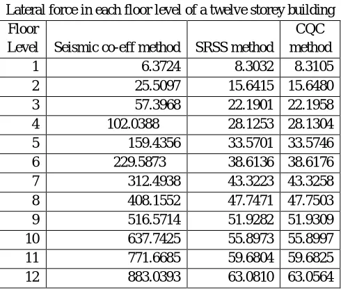
[image:19.612.184.429.351.559.2]The lateral forces at each floor level determined by all the methods obtained as output from MATLAB program is presented here in the table below:
Table 7.1
Lateral force in each floor level of a twelve storey building Floor
Level Seismic co-eff method SRSS method
CQC method 1 6.3724 8.3032 8.3105 2 25.5097 15.6415 15.6480 3 57.3968 22.1901 22.1958 4 102.0388 28.1253 28.1304 5 159.4356 33.5701 33.5746 6 229.5873 38.6136 38.6176 7 312.4938 43.3223 43.3258 8 408.1552 47.7471 47.7503 9 516.5714 51.9282 51.9309 10 637.7425 55.8973 55.8997 11 771.6685 59.6804 59.6825 12 883.0393 63.0810 63.0564
It is observed from the Table 7.1 that the lateral force at various floor levels as per Square Root of Sum of Squares (SRSS) method and Combined Quadratic Combination (CQC) method were almost equal while that by the Seismic co-efficient method is negligibly small for lower floors and deviate very much from the other two methods. But, the deviation reduces for higher floors and becomes the largest among the three values at the roof level.
VIII. ANALYSIS AND DESIGN OF MULTI STOREYED RC FRAME
nodal loads for each column. When earthquake forces are considered on structure, these shall be combined as per 8.2 where the terms DL, LL and EL stands for response quantities due to dead load, live load and designed earthquake load respectively. The column and beam size are entered as the member property.
The analysis of the frame is done for all the zones in India using the load calculated for various zones respectively. The analysis of the structure results in the bending moment and shear force diagram of the frame. For every zone the structure is analysed for both Ordinary moment resisting frame(R=3) and special moment resisting frame(R=5)
A. design of multi storeyed building using staad.pro
After analysing the frame for various zones varying the response reduction factor the frame, using M25 concrete and Fe 415 steel as per IS 456 The parameters that are defined for concrete design are compressive strength of steel for main bars (fy(main)),yield strength of steel for secondary bars(fy(sec)), yield strength of concrete (fc), maximum and minimum values of the size of bars to be used in the design. The members spanning parallel to X and Z direction are designed as beam. The members parallel to Y direction are designed as columns. After the design is performed the no of bars or the spacing of the bars for all the columns and beams are described. The total quantity of concrete in m3 and the total quantity of steel in Newton is obtained finally as the result of the design.
B. Load Combination
In the limit state design of reinforced concrete structures the following load combinations shall be accounted for:
1) 1.5(DL+LL)
2) 1.2(DL+LL+ELx)
3) 1.2(DL+LL+ELy)
4) 1.2(DL+LL-ELx)
5) 1.2(DL+LL-ELy)
6) 1.5(DL+ELx)
7) 1.5(DL+ELy)
8) 1.5(DL-ELx)
9) 1.5(DL-ELy)
10) 0.9DL+1.5ELx
11) 0.9DL+1.5Ely
12) 0.9DL-1.5ELx
13) 0.9DL-1.5Ely
C. Evaluation Of Lateral Force By Seismic Co-Efficient Method Using Matlab Program
The design lateral force as per seismic co-efficient method obtained from matlab is presented in table 8.31 and 8.32. Then the lateral force to be applied at each node for the analysis in staad.pro.
8.3.1 AT EACH FLOOR FOR SMRF
FLOOR LEVEL ZONE 2 ZONE 3 ZONE 4 ZONE 5
ROOF 704.20 780.62 1170.9 1756.4
XI FLOOR 616.45 683.35 1025 1537.5
X FLOOR 509.47 564.75 847.1 1270.7
IX FLOOR 412.67 457.45 686.2 1029.3
VIII FLOOR 326.06 361.44 542.2 813.2
VII FLOOR 249.64 276.72 415.1 622.6
VI FLOOR 183.40 203.311 305 457.5
V FLOOR 127.36 141.18 211.8 317.7
IV FLOOR 81.51 90.36 135.5 203.3
III FLOOR 45.85 50.82 76.2 114.4
II FLOOR 20.38 22.59 33.9 50.8
GROUND FLOOR 5.09 5.64 8.5 12.7
8.3.2 At each floor for OMRF
FLOOR LEVEL ZONE 2 ZONE 3 ZONE 4 ZONE 5
ROOF 813.15 1301 1951.6 2927.3
XI FLOOR 711,82 1138.9 1708.4 2562.6
X FLOOR 588.28 941.3 1411.9 2117.8
IX FLOOR 476.51 762.4 1143.6 1715.4
VIII FLOOR 376.50 602.4 903.6 1355.4
VII FLOOR 288.26 461.2 691.8 1037.7
VI FLOOR 211.78 338.9 508.3 762.4
V FLOOR 147.07 235.3 353 529.5
IV FLOOR 94.12 150.6 225.9 338.9
III FLOOR 52.94 84.7 127.1 190.6
II FLOOR 23.53 37.7 56.5 84.7
GROUNDFLOOR 5.88 9.4 14.1 21.2
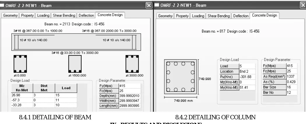
D. Structural Design Of Beam And Column
A sample output for structural design for a beam and column are presented below:
8.4.1 DETAILING OF BEAM 8.4.2 DETAILING OF COLUMN
IX. RESULTS AND DISCUSSIONS
[image:22.612.48.573.102.315.2]The results of seismic analysis had already been presented in Chapter 8. The quantity of steel and concrete obtained from STAAD. Pro design for all the frames and the comparative cost is also presented here
TABLE 9.1 TOTAL QUANTITY OF STEEL AND CONCRETE Zone R Concrete in m3 Steel in N
Normal Design
... 1635 1142635
II 3 2111.8 1328618.3
II 5 2111.8 1267647
III 3 2521.8 1250723
III 5 2521.8 1148455.5
IV 3 2521.8 1567835.5
IV 5 2521.8 1348444
V 3 2743.2 1722614.2
V 5 3030.8 1652322.6
A. Cost Evaluation
For ordinary structure (multi-storey building)without considering earthquake forces, the approximate cost of construction is arrived at as follows
Total cost = (Total Area in m2) x Cost per m2 x No Of Storey = (21 x 21) x 10000 x 12
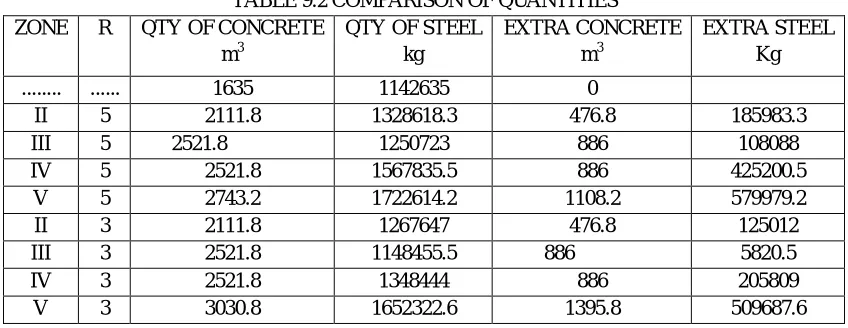
For estimating the increase in cost of construction of the earthquake resistant frame, the extra quantity of steel and concrete is calculated and presented in Table 9.2
TABLE 9.2 COMPARISON OF QUANTITIES ZONE R QTY OF CONCRETE
m3
QTY OF STEEL kg
EXTRA CONCRETE m3
EXTRA STEEL Kg
... ... 1635 1142635 0
II 5 2111.8 1328618.3 476.8 185983.3
III 5 2521.8 1250723 886 108088
IV 5 2521.8 1567835.5 886 425200.5
V 5 2743.2 1722614.2 1108.2 579979.2
II 3 2111.8 1267647 476.8 125012
III 3 2521.8 1148455.5 886 5820.5
IV 3 2521.8 1348444 886 205809
V 3 3030.8 1652322.6 1395.8 509687.6
1) Cost Comparison For Different Zones
Cost of 1 Tonne of steel = Rs 45000.00 Cost per m3 of concrete = Rs 5000.00
Total cost for various zones are worked out as follows Example : Zone V - R =5
Extra concrete = 2743.2-1635 = 1108.2 m3
Extra Steel = 1722614.2-1142635 = 579979.2 Kg
= 579.9792 tonne Extra Cost = (1108.2 X 5000)+(579.9792 X 45000)
= 316.39 lakhs
Total Cost = 529.9 + 316.39= 846.29 lakhs
TABLE 9.3 TOTAL COST OF THE BUILDING
ZONE EXTRA CONCRETE EXTRA STEEL EXTRA COST TOTAL COST IN LAKHS
... 0 595
II 476.8 185983.3 107 702
III 886 108088 92.93 688
IV 886 425200.5 235.64 831
V 1108.2 579979.2 316.4 912
II 476.8 125012 80.09 675
III 886 5820.5 46.91 642
IV 886 205809 136.91 732
Fig: 9.1 COMPARISON OF COST IN LAKHS
[image:24.612.144.470.292.721.2]The above Fig 9.1 indicates the cost in lakhs in all the zones considering both ordinary and special moment resisting frames by taking zones in x-axis and cost in lakhs in y-axis.
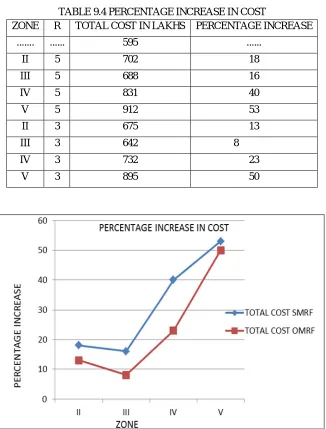
TABLE 9.4 PERCENTAGE INCREASE IN COST
ZONE R TOTAL COST IN LAKHS PERCENTAGE INCREASE
... ... 595 ...
II 5 702 18
III 5 688 16
IV 5 831 40
V 5 912 53
II 3 675 13
III 3 642 8
IV 3 732 23
V 3 895 50
From the above plot it is inferred that there is only a slight increase in the total cost for zones upto IV (ie 5% to 9%). The percentage increase for zone V is 15% and 22% respectively for SMRF and OMRF.
X. CONCLUSION
From the results of seismic analysis of a twelve storeyed RC frame using MATLAB it is found that the lateral force at the lower floors by Seismic co-efficient method is much lower than that of Response Spectrum method. But the difference between the values of Response spectrum method and Seismic co-efficient method reduces for higher floors and the lateral force at the roof level became the highest in seismic co-efficient method. From the analysis and design of the OMRF and SMRF in various earthquake zones using STAAD.Pro it is found that there is increase in cost of 8% to 40% for both the type of construction in zone II to IV from the conventional frame. While increase in cost of construction in zone V is 50 % and 53% respectively for SMRF and OMRF. Hence it is concluded that considering the safety of men and material multi-storeyed RC frames in all earthquake zones in India could be designed as a Special Moment Resisting Frame.
REFERENCES
[1] T.T. Soong, and G.F. Dargush, “Passive energy dissipation systems in structural engineering,” J. Wiley & Sons, Chichester, England, 1997.
[2] C. Christopoulos, and A. Filiatrault, “Principles of passive supplemental damping and seismic isolation,” IUSS Press, Istituto Universitario di Studi Superiori di Pavia (Italy), 2006.
[3] F. Mazza, and A. Vulcano, “Sistemi di controllo passivo delle vibrazioni,” in Progettazione sismo-resistente di edifici in cemento armato, Città Studi Edizioni, Italy, 2011, vol. 11, pp. 525-575.
[4] F. Mazza, A. Vulcano, M. Mazza, and G. Mauro. “Modeling and nonlinear seismic analysis of framed structures equipped with damped braces,” Recent Researches in Information Science and Applications. WSEAS 2013, Milan, Italy, January 9-11, 2013, ISBN: 978-1-61804- 150-0, ISSN: 1790-5109.
[5] F.C. Ponzo, A. Di Cesare, D. Nigro, A. Vulcano, F. Mazza, M. Dolce, C. Moroni, “JET-PACS project: dynamic experimental tests and numerical results obtained for a steel frame equipped with hysteretic damped chevron braces,” Journal of Earthquake Engineering, 2012, vol. 16, pp. 662-685.
[6] J. Molina, S. Sorace, G. Terenzi, G. Magonette, and B. Viaccoz, “Seismic tests on reinforced concrete and steel frames retrofitted with dissipative braces,” Earthquake Engineering and Structural Dynamics, 2004, vol. 33(12), pp. 1373-1394.
[7] A. Baratta, I. Corbi, O. Corbi, R.C. Barros, and R. Bairrão, “Shaking table experimental researches aimed at the protection of structures subject to dynamic loading,” The Open Construction and Building Technology Journal, 2012, vol. 6, pp. 355-360.
[8] Kazuhiko Kawashima, Shigeki Unjoh ” Seismic Response Control of Bridges by Variable Dampers” ASCE Journal of Structural Engineering” Paper No 9, Vol. 120, September 1994 pp. 2583 - 2600.
[9] Parulekar.Y.M, Reddy.G.R, Vaze.K.K, Ghosh.A.K, Kushwaha.H.S and Ramesh Babu.R” Seismic response analysis of RCC structure with yielding dampers using linearization techniques”, Nuclear Engineering and Design, Paper No. 239 August 2009, Vol.23 pp. 3054–3061.
[10] Rashidi.S and Ala Saadeghvaziri.M ”Seismic Modeling of Multi Span simply supported Bridge using ADINA” Computers and Structures, Vol 64, March 1997, pp.1025-1039.
[11] Sevasti. D, Tegou, Stergios. A. Mitoulis ,and Ioannis A. Tegos(2010)”An unconventional earthquake resistant abutment with transversely directed R/C walls” Engineering Structures, Vol. 32 September 2010, pp. 3801–3816.