A statistical approach for identifying differential distributions in single cell RNA seq experiments

M E T H O D

Open Access

A statistical approach for identifying

differential distributions in single-cell RNA-seq

experiments

Keegan D. Korthauer

, Li-Fang Chu

, Michael A. Newton

, Yuan Li

, James Thomson

, Ron Stewart

and Christina Kendziorski

Abstract

The ability to quantify cellular heterogeneity is a major advantage of single-cell technologies. However, statistical methods often treat cellular heterogeneity as a nuisance. We present a novel method to characterize differences in expression in the presence of distinct expression states within and among biological conditions. We demonstrate that this framework can detect differential expression patterns under a wide range of settings. Compared to existing approaches, this method has higher power to detect subtle differences in gene expression distributions that are more complex than a mean shift, and can characterize those differences. The freely available R package scDD implements the approach.

Keywords: Single-cell RNA-seq, Differential expression, Cellular heterogeneity, Mixture modeling

Background

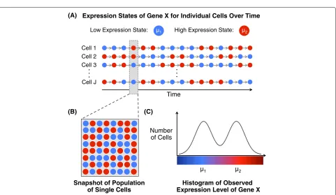
Coordinated gene expression is fundamental to an organ-ism’s development and maintenance, and aberrations are common in disease. Consequently, experiments to mea-sure expression on a genome-wide scale are pervasive. The most common experiment involves the quantification of mRNA transcript abundance averaged over a popu-lation of thousands or millions of cells. These so-called traditional, or bulk, RNA-seq experiments have proven useful in a multitude of studies. However, because bulk RNA-seq does not provide a measure of cell-specific expression, many important signals go unobserved. A gene that appears to be expressed at a relatively constant level in a bulk RNA-seq experiment, for example, may actually be expressed in sub-groups of cells at levels that vary substantially (see Fig. 1).

Single-cell RNA-seq (scRNA-seq) facilitates the mea-surement of genome-wide mRNA abundance in individ-ual cells, and as a result, provides the opportunity to study the extent of gene-specific expression heterogeneity

*Correspondence: [email protected]

4_{Department of Biostatistics, University of Wisconsin, 53706 Madison, WI, USA} 5_{Department of Statistics, University of Wisconsin, 53706 Madison, WI, USA} Full list of author information is available at the end of the article

within a biological condition, and the impact of changes across conditions. Doing so is required for discovering novel cell types [1, 2], for elucidating how gene expression changes contribute to development [3–5], for understand-ing the role of cell heterogeneity on the immune response [6, 7] and cancer progression [6, 8–10], and for predict-ing the response to chemotherapeutic agents [11–13]. Unfortunately, the statistical methods available for char-acterizing gene-specific expression within a condition and for identifying differences across conditions in scRNA-seq are greatly limited, largely because they do not fully accommodate the cellular heterogeneity that is prevalent in single-cell data.

To identify genes with expression that varies across bio-logical conditions in an scRNA-seq experiment, a num-ber of early studies used methods from bulk RNA-seq [4, 10, 12, 14, 15]. In general, the methods assume that each gene has a latent level of expression within a biolog-ical condition, and that measurements fluctuate around that level due to biological and technical sources of vari-ability. In other words, they assume that gene-specific expression is well characterized by a unimodal distribu-tion within a condidistribu-tion. Further, tests for differences in expression to identify so-called differentially expressed (DE) genes amount to tests for shifts in the unimodal

Snapshot of Population of Single Cells

Histogram of Observed Expression Level of Gene X

Number of Cells

(A)

(B) (C)

Expression States of Gene X for Individual Cells Over Time

Low Expression State:

µ1 µ2

Time

Cell 1 Cell 2 Cell 3

Cell J

µ1 High Expression State: µ2

Fig. 1Schematic of the presence of two cell states within a cell population that can lead to bimodal expression distributions.aTime series of the underlying expression state of gene X in a population of unsynchronized single cells, which switches back and forth between a low and high state with meansμ1andμ2, respectively. The color of cells at each time point corresponds to the underlying expression state.bPopulation of individual cells shaded by expression state of gene X at a snapshot in time.cHistogram of the observed expression level of gene X for the cell population in (b)

tributions across conditions. A major drawback of these approaches in the single-cell setting is that, due to both biological and technical cell-to-cell variability, there is often an abundance of cells for which a given gene’s expression is unobserved [7, 16, 17] and, consequently, unimodal distributions are insufficient.

To address this, a number of statistical methods have been developed recently to accommodate bimodal-ity in scRNA-seq data [17, 18]. In these mixture-model based approaches, one component distribution accommodates unobserved, or dropout, measurements (which include zero and, optionally, thresholded low-magnitude observations) and a second unimodal com-ponent describes gene expression in cells where expres-sion is observed. Although these approaches provide an advance over unimodal models used in bulk, they are insufficient for characterizing multi-modal expres-sion data, which is common in scRNA-seq experiments (see Fig. 2).

Specifically, a number of studies have shown that many types of heterogeneity can give rise to multiple expression modes within a given gene [19–23]. For example, there are often multiple states among expressed genes [19, 20, 22] (a schematic is shown in Fig. 1). The transition between cell states may be primarily stochastic in nature and result

from expression bursts [24, 25], or result from positive feedback signals [19, 23, 26]. Beyond the existence of mul-tiple stable states, mulmul-tiple modes in the distribution of expression levels in a population of cells may also arise when the gene is either oscillatory and unsynchronized, or oscillatory with cellular heterogeneity in frequency, phase, and amplitude [21, 23].

0.00 0.25 0.50 0.75 1.00

1 2 3+

Number of Modes

Propor

tion of genes (or tr

anscr

ipts) _Dataset

GE.50

GE.75

GE.100

LC.77

H1.78

DEC.64

NPC.86

H9.87

Modality of Bulk (Reds) vs Single−cell (Blues) RNA−seq datasets

Fig. 2Comparison of modality in bulk versus single cells. Bar plot of the proportion of genes (or transcripts) in each dataset where the log-transformed nonzero expression measurements are best fit by a 1, 2, or 3₊mode normal mixture model (where 3₊denotes 3 or more). Modality is determined using a Bayesian information selection criterion with filtering (see “Partition estimation”).Red shadesdenote bulk RNA-seq datasets, andblue shadesdenote single-cell datasets. The number following each dataset label indicates the number of samples present (e.g.,GE.50 is a bulk dataset with 50 samples). DatasetsGE.50,GE.75, andGE.100are constructed by randomly sampling 50, 75, and 100 samples from GEUVADIS [56]. DatasetLCconsists of 77 normal samples from the TCGA lung adenocarcinoma study [57]. For details of the single-cell datasets, see “Methods”

Traditional DE

µ1 µ2

(A) DP

µ1 µ2

(B)

DM

µ1 µ2

(C) DB

µ1 µ3 µ2

(D)

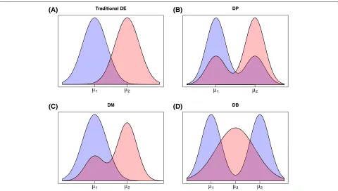
Here we develop a Bayesian modeling framework, scDD, to facilitate the characterization of expression within a biological condition, and to identify genes with differential distributions (DDs) across conditions in an scRNA-seq experiment. A DD gene may be classified as DE, DM, DP, or both DM and differential means of expression states (abbreviated DB). Figure 3 provides an overview of each pattern. Simulation studies suggest that the approach provides improved power and precision for identifying differentially distributed genes. Additional advantages are demonstrated in a case study of human embryonic stem cells (hESCs).

Results and discussion Human embryonic stem cell data

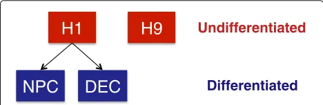
scRNA-seq data were generated in the James Thomson Lab at the Morgridge Institute for Research (see “Methods” and [30] for details). Here we analyze data from two undifferentiated hESC lines: the male H1 line (78 cells) and the female H9 line (87 cells). In addition, we include data from two differentiated cell types that are both derived from H1: definitive endoderm cells (DECs, 64 cells) and neuronal progenitor cells (NPCs, 86 cells). The relationship between these four cell types is summa-rized by the diagram in Fig. 4. As discussed in the case study results, it is of interest to characterize the differ-ences in distributions of gene expression among these four cell types to gain insight into the genes that regulate the differentiation process.

Publicly available human myoblast and mouse embryonic stem cell data

We also apply our method to two publicly available scRNA-seq datasets to determine which genes are differ-entially distributed following stimulation or inhibition of differentiation via a specialized growth medium. Using data from [31], we compare gene expression of human myoblast cells cultured in standard growth medium (T0, 96 cells) with those treated with differentiation-inducing medium for 72 hours (T72, 84 cells). Additionally, we use data from [32] to compare the gene expression of

Undifferentiated

Differentiated

H1

NPC

DEC

H9

Fig. 4Relationship of cell types used in hESC case study.H1andH9 are undifferentiated hESC lines.NPC(neuronal progenitor cells) and DEC(definitive endoderm cells) are differentiated cell types derived fromH1.DECdefinitive endoderm cell,NPCneuronal progenitor cell

mouse embryonic stem cells (mESCs) cultured in stan-dard medium (Serum + LIF, 93 cells) with those cultured on differentiation-inhibiting medium (2i + LIF, 94 cells).

Simulated data

We evaluate model performance using log-transformed count data simulated from mixtures of negative bino-mial distributions. The analysis of log-transformed counts from bulk RNA-seq has been shown to perform as well as utilizing count-based modeling assumptions [33, 34]. Recent scRNA-seq analyses have also assumed the nor-mality of log-transformed nonzero measurements [7, 18]. For each simulated dataset, 10,000 genes were simulated for two conditions with four different sample size settings (50, 75, 100, and 500 cells in each condition). The majority of the genes (8000) were simulated out of the same model in each condition, and the other 2000 represent genes with the four types of DD outlined in Fig. 3. The 2000 DD genes were split equally into the following four categories:

• DE: single component with a different mean in each

condition

• DP: two components in each condition with equal

component means across conditions; the proportion in the low mode is 0.33 for condition 1 and 0.66 for condition 2

• DM: single component in condition 1; two

components in condition 2 with one overlapping component. Half of the condition 2 cells belong to each mode

• DB: single component in condition 1; two

components in condition 2 with no overlapping components. The mean of condition 1 is half-way between the means in condition 2. Half of the cells in condition 2 belong to each mode

to be common across components for a given gene and condition). More details are provided in “Methods”.

The scDD modeling framework

LetYg = (yg1,. . .,ygJ) be the log-transformed nonzero expression measurements of gene g in a collection of

J cells from two biological conditions. We assume that measurements have been normalized to adjust for tech-nical sources of variation including amplification bias and sequencing depth. Under the null hypothesis of equiva-lent distributions (i.e., no dependence on condition), we letYgbe modeled by a conjugate Dirichlet process mixture (DPM) of normals (see “Methods” for more details). Gene

gmay also have expression measurements of zero in some cells; these are modeled as a separate distributional com-ponent (see “Differential proportion of zeroes” for more details).

Ultimately, we would like to calculate a Bayes factor for the evidence that the data arises from two independent condition-specific models (DDs) versus one overall model that ignores condition (equivalent distributions or EDs). LetMDDdenote the DD hypothesis, andMEDdenote the

equivalent distribution hypothesis. A Bayes factor in this context for genegwould be:

BFg=

f(Yg|MDD)

f(Yg|MED)

wheref(Yg|M)denotes the predictive distribution of the observations from gene g under the given hypothesis. In general, there is no analytical solution for this dis-tribution under the DPM model framework. However, under the product partition model (PPM) formulation (see “Methods” for more details), we can get a closed form solution forf(Yg,Zg|M), whereZgrepresents a partition (or clustering) of samples to mixture components. As the partition Zg cannot be integrated out, we introduce an approximate Bayes factor score:

Scoreg=log

f(Yg,Zg|MDD)

f(Yg,Zg|MED)

=log

fC1(YgC1,ZCg1)fC1(YgC2,ZCg2)

fC1,C2(Yg,Zg)

whereC1 andC2 denote conditions 1 and 2, respectively, and the score is evaluated at the partition estimateZˆg. A high value of this score presents evidence that a given gene is differentially distributed. The significance of the score is assessed via a permutation test. Specifically, condition labels are permuted and partition estimates are obtained within the new conditions. For each permuted dataset, the Bayes factor score is calculated; the default in scDD is 1000 permutations. For each gene, an empiricalpvalue is calculated, and the false discovery rate (FDR) is controlled for a given target value using the method of [35].

If covariates are available, instead of permuting the observed values, the relationship between the clustering and covariates can be preserved by permuting the residu-als of a linear model that includes the covariate and using the fitted values [36]. As pointed out by [18], the cellu-lar detection rate is a potential confounder variable, so the permutation procedure in the case studies is adjusted in this manner. If other known confounders exist and are measured, these can also be incorporated in the same manner. Note that while this procedure adjusts for covari-ates that affect mean expression levels, it does not adjust for covariate-specific effects on variance. The sensitivity of the approach to various levels of nonlinear confound-ing effects is evaluated in a simulation study presented in Additional file 1: Section 2.3.

Classification of significant DD genes

For genes that are identified as DD by the Bayes factor score, of interest is classifying them into four categories that represent the distinct DD patterns shown in Fig. 3. To classify the DD genes into these patterns (DE, DM, DP, and DB), scDD utilizes the conditional posterior distribu-tion of the component-specific mean parameters given in Eq. 6 (see “Methods”). Posterior sampling is carried out to investigate the overlap of components across conditions. Letc1be the number of components in condition 1,c2the

number of components in condition 2, andcOAthe

num-ber of components overall (when pooling conditions 1 and 2). Only components containing at least three cells are considered to minimize the impact of outlier cells. Note that for interpretability, a DD gene must satisfy:c1+c2≥

cOA ≥ min(c1,c2). These bounds on the overall number

of components represent the two extreme cases: condi-tion 1 does not overlap with condicondi-tion 2 at all, versus one condition completely overlaps with the other. Any cases outside of these boundaries are not readily interpretable in this context. The actions to take for all other possible combinations ofc1,c2, andcOAare detailed in “Methods”.

Differential proportion of zeroes

For those genes that do not show DDs in the nonzero values, scDD allows a user to evaluate whether the pro-portion of zeroes differs significantly between the two conditions. This evaluation is carried out using logistic regression adjusted for the proportion of genes detected in each cell as in [18]. Genes with aχ2_{testpvalue of less than}

0.025 (after adjustment for multiple comparisons using the method of [35]) are considered to have a differential proportion of zeroes (DZ).

Simulation study

simulated data was assessed based on (1) the ability to esti-mate the correct number of components, (2) the ability to detect significantly DD genes, and (3) the ability to classify DD genes into their correct categories. These three cri-teria are explored in the next three sections, respectively. Existing methods for DE analysis are also evaluated for the second criterion.

Estimation of the number of components

We first examine the ability of scDD to detect the correct number of components. Table 1 displays the proportion of bimodal and unimodal simulated genes where the correct number of components was identified. For bimodal genes, results are stratified by component mean distance. It is clear that the ability of the algorithm to identify the cor-rect number of components in bimodal genes improves as the component mean distance or sample size increases. The results for unimodal genes are not as sensitive to sam-ple size; however, the proportion of genes identified as bimodal increases slightly with more samples. We con-clude that the partition estimate is able to detect reliably the true number of components for reasonable sample and effect sizes.

Detection of DD genes

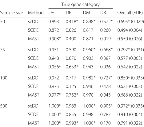
Next, we examine the ability of scDD to identify the non-null genes as significantly DD, and compare it to existing methods, SCDE [17] and MAST [18]. For each method, the target FDR was set at 5 % (see “Methods” for details). The power to detect each gene pattern as DD for all three methods is shown in Table 2. Note that the calculations here are taken before the classification step for scDD, so power is defined as the proportion of genes from each simulated category that are detected as DD. In general, the power to detect DD genes improves with increased sample size for all three methods. Our approach has compara-ble power to SCDE and MAST for DE and DP genes, but higher overall power to detect DM and DB genes. Inter-estingly, SCDE has very low power to detect DP genes, whereas MAST shows very low power to detect DB genes.

Table 1Rate of detection of correct number of components in

simulated data

Bimodal Unimodal

Sample component mean distance_μ

size 2 3 4 5 6

50 0.056 0.196 0.579 0.848 0.922 0.907

75 0.052 0.252 0.719 0.917 0.957 0.908

100 0.050 0.302 0.811 0.950 0.974 0.905

500 0.073 0.417 0.959 0.995 0.991 0.884

Average proportion of simulated bimodal and unimodal genes where the correct number of components was identified, averaged over gene category and condition. Averages are calculated over 20 replications. Standard errors were<0.025 (not shown)

Table 2Power to detect DD genes in simulated data

True gene category

Sample size Method DE DP DM DB Overall (FDR)

50 scDD 0.893 0.418* 0.898* 0.572* 0.695* (0.029)

SCDE 0.872 0.026 0.817 0.260 0.494 (0.004)

MAST 0.908* 0.400 0.871 0.019 0.550 (0.026)

75 scDD 0.951 0.590 0.960* 0.668* 0.792* (0.031)

SCDE 0.948 0.070 0.903 0.387 0.577 (0.003)

MAST 0.956* 0.633* 0.943 0.036 0.642 (0.022)

100 scDD 0.972 0.717 0.982* 0.727* 0.850* (0.033)

SCDE 0.975 0.125 0.946 0.478 0.631 (0.003)

MAST 0.977* 0.752* 0.970 0.045 0.686 (0.022)

500 scDD 1.000* 0.983 1.000* 0.905* 0.972* (0.035)

SCDE 1.000* 0.855 0.998 0.787 0.910 (0.004)

MAST 1.000* 0.993* 1.000* 0.170 0.791 (0.022)

Average power to detect simulated DD genes by true category. Averages are calculated over 20 replications. Standard errors were<0.025 (not shown)

DBboth differential modality and different component means,DDdifferential distribution,DEdifferential expression,DMdifferential modality,DPdifferential proportion,FDRfalse discovery rate. Values followed by * designate which method(s) achieved the highest power to detect DD genes from each particular gene category (as well as overall) for each sample sample size setting

We note that SCDE and MAST do not aim to detect genes with no change in the overall mean level in expressed cells (as in the case of DB genes), so it is expected that scDD will outperform other methods at detecting genes in this category.

Classification of DD genes

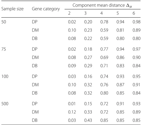
Next, we examine the ability of scDD to classify each DD gene into its corresponding category. Table 3 shows the correct classification rate in each category for DD genes that were correctly identified during the detection step (calculated as the proportion of true positive genes detected as DD for a given category that were classi-fied into the correct category). The classification rates do not depend strongly on sample size, with the exception of DP, which decreases with increasing sample size. This decrease results from an increase in the DD detection rate of DP genes with small component mean distance, which have a lower correct classification rate (as shown below).

Table 3Correct classification rate in simulated data

Gene category

Sample size DE DP DM DB

50 0.719 0.801 0.557 0.665

75 0.760 0.732 0.576 0.698

100 0.782 0.678 0.599 0.706

500 0.816 0.550 0.583 0.646

Average correct classification rate for detected DD genes. Averages are calculated over 20 replications. Standard errors were<0.025 (not shown)

DBboth differential modality and different component means,DDdifferential distribution,DEdifferential expression,DMdifferential modality,DPdifferential proportion

estimation of the number of components. Performance generally increases with sample size, especially at lower values of μ. In general, the ability of the algorithm to classify detected DD genes into their true category is robust when components are well separated and improves with increasing sample size.

Case study: identifying DD genes between hESC types The comprehensive characterization of transcriptional dynamics across hESC lines and derived cell types aims to provide insight into the gene regulatory processes governing pluripotency and differentiation [37–39]. Pre-vious work utilizing microarrays and bulk RNA-seq largely focused on identifying genes with changes in aver-age expression level across a population of cells. By exam-ining transcriptional changes at the single-cell level, we

Table 4Average correct classification rates by component mean

distance

Sample size Gene category Component mean distanceμ

2 3 4 5 6

50 DP 0.02 0.20 0.78 0.94 0.98

DM 0.10 0.23 0.59 0.81 0.89

DB 0.08 0.22 0.59 0.80 0.80

75 DP 0.02 0.18 0.77 0.94 0.97

DM 0.08 0.27 0.69 0.86 0.90

DB 0.09 0.29 0.71 0.83 0.84

100 DP 0.03 0.16 0.74 0.93 0.95

DM 0.10 0.32 0.76 0.87 0.91

DB 0.08 0.32 0.80 0.85 0.84

500 DP 0.01 0.15 0.72 0.91 0.93

DM 0.12 0.33 0.72 0.85 0.89

DB 0.03 0.43 0.85 0.85 0.85

Average correct classification rates stratified byμ. Averages are calculated over 20 replications. Standard errors were<0.025 (not shown)

DBboth differential modality and different component means,DMdifferential modality,DPdifferential proportion

can uncover global changes that are undetectable when averaging over the population. In addition, we gain the ability to assess the level of heterogeneity of key dif-ferentiation regulators, which may lead to the ability to assess variation in pluripotency [40] or the differentiation potential of individual cells.

The number of significant DD genes for each cell type comparison is shown in Table 5 for scDD, SCDE, and MAST. Note that the comparison of H1 and H9 detects the fewest number of DD genes for all three methods, a finding that is consistent with that both of these are undif-ferentiated hESC lines and it is expected that they are the most similar among the comparisons. In all four compar-isons, the number of genes identified by our method is greater than that for SCDE and similar to that for MAST.

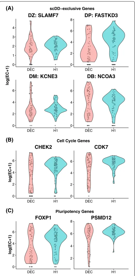
Figure 5a displays top-ranked genes for each category that are not identified by MAST or SCDE for the H1 ver-sus DEC comparison. Among the genes identified exclu-sively by scDD for the H1 versus DEC comparison are

CHEK2, a cell-cycle checkpoint kinase [41], andCDK7, a cyclin-dependent kinase that plays a key role in cell-cycle regulation through the activation of other cyclin-dependent kinases [42]. It has been shown that embryonic stem cells express cyclin genes constitutively, whereas in differentiated cells, cyclin levels are oscillatory [43]. This finding is consistent with the differential modality of the

CDK7 gene shown in Fig. 5b. Similarly, scDD identifies several genes involved in the regulation of pluripotency that are not identified by the other two methods (Fig. 5c). For example,FOXP1exhibits alternative splicing activity in hESCs, stimulating expression of several key regula-tors of pluripotency [44]. ThePSMD12 gene encodes a subunit of the proteasome complex that is vital to the maintenance of pluripotency and has shown decreased expression in differentiating hESCs [45]. Both of these genes are also differentially distributed between H1 and the other differentiated cell type, NPC.

In general, the vast majority of the genes found exclusively by scDD are categorized as something other

Table 5Number of DD genes identified in the hESC case study

data for scDD, SCDE, and MAST

scDD

Comparison DE DP DM DB DZ Total SCDE MAST

H1 vs NPC 1686 270 902 440 1603 5555 2921 5887

H1 vs DEC 913 254 890 516 911 5295 1616 3724

NPC vs DEC 1242 327 910 389 2021 5982 2147 5624

H1 vs H9 260 55 85 37 145 739 111 1119

Note that the total for scDD includes genes detected as DD but not categorized

0 1 2 3 4

DEC H1

DZ: SLAMF7

0 2 4 6 8

DEC H1

DP: FASTKD3

0 2 4 6

DEC H1

DM: KCNE3

0 2 4 6

DEC H1

DB: NCOA3

0 2 4 6

DEC H1

CHEK2

0 2 4 6

DEC H1

CDK7

0 2 4 6

DEC H1

FOXP1

2 4 6 8

DEC H1

PSMD12

log(EC+1)

(A) scDD−exclusive Genes

log(EC+1)

log(EC+1)

(B)

(C)

Cell Cycle Genes

Pluripotency Genes

Fig. 5Violin plots (smoothed non-parametric kernel density estimates) for Differentially Distributed genes identified between H1 and DEC. Individual observations are displayed with jitter. Within a condition, points with the same shape are predicted to belong to the same component.ascDD-exclusive genes: representative genes from each category (DZ, DP, DM, and DB) that are not detected by MAST or SCDE. Selected genes are top-ranked by permutationpvalue in each category (DP, DM, and DB) or had a significant_χ2_{test for a difference} in the proportion of zeroes (DZ).bCell-cycle genes: DD genes involved in cell-cycle regulation (not detected by MAST or SCDE).c Pluripotency genes: DD genes involved in pluripotency regulation (not identified by MAST or SCDE).DBboth differential modality and different component means,DDdifferential distribution,DEC definitive endoderm cell,DMdifferential modality,DPdifferential proportion,DZdifferential zeroes

than DE (ranging from 98.3 to 100 % in the three case studies, see Additional file 1: Table S6), which suggests that they are predominantly characterized by differences that are more complex than the traditional DE pattern. The genes identified by MAST but not scDD are over-whelmingly characterized as those with a weak signal in both the nonzero and zero components (see Additional file 1: Figure S9), which can be difficult to interpret (see Additional file 1: Section 3 for more details).

Additional case studies

We also applied scDD and MAST to two additional case studies (the numbers of significant DD genes for each comparison are displayed in Table 6). SCDE was not used to analyze these datasets since it is intended for use on raw count data and the processed data made available by the authors of [31, 32] were already normalized by FPKM and TPM, respectively. Like the results of the hESC case study, MAST and scDD identify similar numbers of sig-nificant genes. The genes that scDD finds exclusively are predominantly characterized by something other than a mean shift, a result which is also consistent with the hESC case study (see Additional file 1: Table S7).

Advantages and limitations of the approach

We stress that our approach is inherently different from a method that detects traditional DE, such as [17] and [18], which aim to detect a shift in the mean of the expressed values. In addition to identifying genes that have DDs across conditions, our modeling framework allows us to identify subpopulations within each condition that have differing levels of expression of a given gene (i.e., which cells belong to which component). For such genes, the par-tition estimates automatically provide an estimate of the proportion of cells in each condition that belong to each subpopulation. We also do not require specification of the total number of components, which can vary for each gene.

When applied to cells at different differentiation stages, this information may provide insight into which genes are responsible for driving phenotypic changes. The gene in Fig. 3b, for example, shows a DP of cells across

Table 6Number of DD genes identified in the myoblast and

mESC case studies for scDD and MAST

scDD

Comparison DE DP DM DB DZ Total MAST

Myoblast: T0 vs T72 312 44 200 36 1311 2134 2904

mESC: Serum vs 2i 5233 76 1259 1128 670 9130 9706

Note that the total for scDD includes genes detected as DD but not categorized

conditions, which is important to recognize since DP suggests a change in cell-specific responses to signaling [7, 29]. This is in contrast to the DM gene in Fig. 3c, which indicates the presence of a distinct cell type in one condition, but not the other. Recent methods for scRNA-seq [17, 18, 27, 28, 46] may be able to identify genes such as those shown in Fig. 3b–d as differing between conditions. However, our simulations suggest that they would be relatively underpowered to do so, and they would be unable to characterize the change as DP, DM, or DB.

We also show through simulation that our approach can accommodate large sample sizes of several hundreds of cells per condition. Note, however, that the real strength in the modeling framework lies in the ability to characterize patterns of DDs. In the presence of extreme sparsity, this will be a challenge, since the number of nonzero obser-vations in a given gene will be small. If the sample size of nonzero measurements is too small, it will be difficult to infer the presence of multiple underlying cell states. In practice, for larger and more sparse datasets, it is recom-mended to verify that the number of cells expressing a given gene is in the range of the sample sizes considered in this study to utilize fully the available features of scDD. The approach is limited in that adjustments for covari-ates are not directly incorporated into the model. In general, when the relationship between a potential con-founding variable and the quantification of expression is well known (e.g., increased sequencing depth is generally associated with increased expression measurements), this should be accounted for in a normalization procedure. For other covariates that are not as well characterized (e.g., the cellular detection rate and batch effects), residuals can be used in the permutation procedure, though a more unified approach would be desirable. We also note that more com-plex confounding variables may be present in scRNA-seq experiments that are nonlinear in nature (e.g., covariate-specific effects on variance). We show in Additional file 1: Section 2.3 that when these effects are extreme, care must be taken in interpreting DD genes that are uncategorized. Additionally, the approach is limited in that only pair-wise comparisons across biological conditions are fea-sible. While an extended Bayes factor score to test for the dependence of a condition on a partition estima-tion for more than two condiestima-tions would be straightfor-ward, the classification into meaningful patterns would be less so, and work is underway in that direction. Finally, we note that while the genes identified by scDD may prove useful in downstream analysis, inter-pretability is limited as partitions are estimated inde-pendently for each gene and consequently do not pro-vide a unified clustering of cells based on global gene expression changes. Extensions in this direction are also underway.

Conclusions

To our knowledge, we have presented the first statistical method to detect differences in scRNA-seq experiments that explicitly accounts for potential multi-modality of the distribution of expressed cells in each condition. Such multi-modal expression patterns are pervasive in scRNA-seq data and are of great interest, since they represent biological heterogeneity within otherwise homogeneous cell populations; differences across conditions imply dif-ferential regulation or response in the two groups. We have introduced a set of five interesting patterns to sum-marize the key features that can differ between two con-ditions. Using simulation studies, we have shown that our method has comparable performance to existing methods when differences (mean shifts) exist between unimodal distributions across conditions, and it outper-forms existing approaches when there are more complex differences.

Methods

Software implementations and applications

All analyses were carried out using R version 3.1.1 [47]. The method MAST [18] was implemented using the MAST R package version 0.931, obtained from GitHub at https://github.com/RGLab/MAST. The adjustment for cellular detection rate as recommended in [18] was included in the case study, but not in the simulation study (only the normal component of the test was con-sidered here since no difference in dropout rate was sim-ulated). The method SCDE [17] was implemented using the scde R package version 1.0, obtained from http:// pklab.med.harvard.edu/scde/index.html. No adjustment for cellular detection rate was carried out since SCDE cannot accommodate covariates. Since SCDE requires raw integer counts as input, and expected counts are non-integer valued, the ceiling function was applied to the unnormalized counts. For each approach, the tar-get FDR was controlled at 5 %. Specifically, both MAST and SCDE provide gene-specific p values and use the method of [35] to control FDR. We followed the same procedure here.

datasets for SCDE (MAST) ranged from approximately 3 to 30 (0.5 to 5) minutes across the different sample sizes.

hESC culture and differentiation

All cell culture and scRNA-seq experiments were con-ducted as described previously [30, 48]. Briefly, undif-ferentiated H1 and H9 hESCs were routinely maintained at the undifferentiated state in E8 medium on Matrigel (BD Bioscience) coated tissue culture plates with daily medium feeding [49]. HESCs were passaged every 3 to 4 days with 0.5 mM ethylenediaminetetraacetic acid (EDTA) in phosphate-buffered saline (PBS) at 1:10 to 1:15 ratio for maintenance. H1 were differ-entiated according to previously established protocols [50, 51]. All the cell cultures performed in our laboratory have been routinely tested as negative for mycoplasma contamination.

For DECs, H1 cells were individualized with Accutase (Life Technologies), seeded in E8 with BMP4 (5 ng/ml), Activin A (25 ng/ml) and CHIR99021 (1 μM) for the first 2 days, then withdraw CHIR99021 for the remain-ing period of differentiation. DECs were harvested at the end of day 5, and sorted for the CXCR4-positive popu-lation for scRNA-seq experiments. For NPCs, the undif-ferentiated H1-SOX2-mCherry reporter line was treated with 0.5 mM EDTA in PBS for 3 to 5 min and seeded in E6 (E8 minus FGF2, minus TGFβ1), with 2.5μg/ml insulin, SB431542 (10μM) and 100 ng/ml Noggin. NPCs were harvested and enriched at the end of day 7, after sorting for the Cherry-positive population for scRNA-seq experiments. All differentiation media were changed daily.

Read mapping, quality control, and normalization

For each of the cell types studied, expected counts were obtained from RSEM [52]. In each condition there are a maximum of 96 cells, but all have fewer than 96 cells due to removal by quality control standards. Some cells were removed due to cell death or doublet cell capture, indi-cated by a post cell capture image analysis as well as a very low percentage of mapped reads. For more details on read mapping and quality control, see [30, 48]. DESeq normal-ization [53] was carried out using theMedianNorm func-tion in theEBSeqR package [54] to obtain library sizes. The library sizes were applied to scale the count data. Further, genes with a very low detection rate (detected in fewer than 25 % of cells in either condition) are not considered.

Publicly available scRNA-seq datasets

Processed FPKM-normalized data from human myoblast cells [31] were obtained from GEO [55] using acces-sion number GSE52529. In this study, we examined

the set of cells cultured on standard growth medium (samples labeled with T0) as well as those treated with differentiation-inducing medium for 72 h (sam-ples labeled with T72). Processed TPM-normalized data from mESCs [32] were also obtained from GEO under accession number GSE60749. In this study, we examined the samples labeled as mESC (cultured in standard medium), along with the samples labeled as TwoiLIF (cultured in 2i + LIF differentiation-inhibitory medium).

Publicly available bulk RNA-seq datasets

The modality of the gene expression distributions in bulk RNA-seq was explored using large, publicly avail-able datasets and the results are displayed in Fig. 2. In this figure, the red bars depict the bulk RNA-seq results, and datasets are labeled according to their source and sample size. Datasets GE.50, GE.75, and GE.100 are constructed by randomly sampling 50, 75, and 100 samples from GEUVADIS [56] to obtain sam-ple sizes comparable to the single-cell sets under study (obtained from the GEUVADIS consortium data browser at www.ebi.ac.uk/arrayexpress/files/E-GEUV-1/analysis_ results/GD660.GeneQuantCount.txt.gz). Dataset LC con-sists of 77 normal lung tissue samples from the TCGA lung adenocarcinoma study [57] (obtained from GEO [55] using accession number GSE40419). All datasets were normalized using DESeq normalization [53] except for LC, for which the authors supplied values already normal-ized by RPKM.

Mixture model formulation

Dirichlet process mixture of normals

LetYc

g = (ycg1,. . .,ycgJc) be the log-transformed nonzero

expression measurements of geneg for a collection ofJc cells in conditioncout of 2 total conditions. For simplic-ity of presentation, we drop the dependency ongfor now, and let the total number of cells with nonzero measure-ments be J. We assume that under the null hypothesis of equivalent distributions (i.e., no dependency on condi-tion),Y = {Yc}c=1,2can be modeled by a conjugate DPM

of normals given by

yc_j ∼N(μj,τj) μj,τj∼G

G∼DP(α,G0)

G0=NG(m0,s0,a0/2, 2/b0)

(1)

where DP is the Dirichlet process with base distribution

G0and precision parameterα,N(μj,τj)is the normal dis-tribution parameterized with mean μj and precision τj (i.e., with varianceτ_j−2), and NG(m0,s0,a0/2, 2/b0)is the

components [unique values among(μ,τ) = {μj,τj}Jj=1].

Note that two observations indexed byjandj belong to the same component if and only if(μj,τj)=(μj,τj).

Product partition models

The posterior distribution of(μ,τ)is intractable even for moderate sample sizes. This is because the number of pos-sible partitions (clusterings) of the data grows extremely rapidly as the sample size increases (according to the Bell number). However, if we letZ = (z1,. . .,zJ)be the vec-tor of component memberships of genegfor all samples, where the number of unique Z values is K, the proba-bility density ofY conditional onZ can be viewed as a PPM [58, 59]. Thus, it can be written as a product over all component-specific densities:

f(Y|Z)=

K

k=1

f(y(k)) (2)

where y(k) is the vector of observations belonging to componentkandf(y(k))is the component-specific distri-bution after integrating over all other parameters. In the conjugate normal-gamma setting, this has a closed form given by

f(y(k))∝ (ak/2)

(bk/2)ak/2

s−_k1/2. (3)

The posterior for the parameters(μk,τk)conditional on the partition is

(μk,τk)|Y,Z∼NG(mk,sk,ak/2, 2/bk). (4)

The posterior parameters (m_k, s_k, a_k, b_k) also have a closed form due to the conjugacy of the model given by Eq. 1. These parameters are given by

sk=s0+n(k)

mk=

s0m0+y(k)

sk

ak=a0+n(k)

bk=b0+

(y(k))2+s0m20−skm2k

(5)

wheren(k) is the number of observations in component

k. It follows that the marginal posterior distribution ofμk conditional on the partition is

μk|Y,Z∼tak

m_k, bk

aksk

(6)

whereta(b,c)denotes the generalized Student’st distribu-tion withadegrees of freedom, noncentrality parameterb, and scale parameterc. The product partition DPM model can be simplified as follows:

yj|zj=k,μk,τk ∼N(μk,τk)

μk,τk ∼NG(m0,s0,a0/2, 2/b0)

z∼ α

K_(α)

(α+J)

K

k=1 (n(k)).

(7)

Then we can obtain the joint predictive distribution of the dataYand partitionZby incorporating Eq. 7:

f(Y,Z)=f(Z)

K

k=1

f(y(k))

∝αK K

k=1

(n(k))(ak/2) (bk/2)ak/2

s−_k1/2.

(8)

Model-fitting

The fitting of the model given in Eq. 7 involves obtain-ing an estimateZˆ of the partition. The goal is to find the partition that yields the highest posterior mass in Eq. 8, referred to as the maximum a posteriori (MAP) partition estimate. Under this modeling framework, the solution for the MAP estimate is not deterministic and several com-putational procedures have been developed utilizing Polya urn Gibbs sampling [60–62], agglomerative greedy search algorithms [63, 64], or an iterative stochastic search [65].

These procedures generally involve evaluation of the posterior at many different candidate partitions, and as such tend to be computationally intensive. To avoid this challenge, we recognize the relation to the corresponding estimation problem in the finite mixture model frame-work, where the partition estimate can be obtained by optimizing the Bayesian information criterion (BIC) of the marginal densityf(Y|Z)[66]. In fact, for certain settings of the prior distribution over partitions, the MAP esti-mate is identical to the estiesti-mate obtained by optimizing the BIC [59]. In practice, even when these settings are not invoked, the performance of partition estimates obtained via BIC optimization show comparable performance (see Additional file 1: Section 1). We obtain the partition esti-mate Zˆ that optimizes the BIC using the Mclust R package [66] and satisfies the criteria for multi-modality described in the next section.

The hyperparameters for the component-specific mean and precision parameters were chosen so as to encode a heavy-tailed distribution over the parameters. Specifi-cally, the parameters were set toμ0 =0,τ02 =0.01,a0=

0.01, andb0 = 0.01. The Dirichlet concentration

param-eter was set toα = 0.01, and choosing this is shown in Additional file 1: Section 1 to be robust to many different settings in a sensitivity analysis.

Partition estimation

criteria. Note that the only constraint imposed on the number of componentsKin the modeling framework is thatK≤J. However, under the sample sizes in this study, we consider only K ≤ 5. The first filtering criterion is based on the notion that a two-component mixture model is not necessarily bimodal [67], and relaxes the require-ment that the MAP estimate corresponds to the model with the lowest BIC. Specifically, for each candidate model fitted by BIC withKcomponents, a split step (ifK = 1, obtain a new partition estimate Zˆ with K = 2 unique elements) or a merge step (if K ≥ 2, obtain a new par-tition estimate Zˆ restricted to K − 1 unique elements) is carried out to generate a new candidate partition. The candidate partition with the larger value ofKbecomes the partition estimate only if the component separation sug-gests multi-modality. Component separation between any pair of components is assessed with the bimodality index (BI) [68]:

BI=2× n1n2 (n1+n2)2

|μ1−μ2| σ

where the component means μ1 and μ2 are estimated

via maximum likelihood, the common within-component standard deviationσis conservatively estimated with the maximum within-component standard deviation among all components, and n1 and n2 are the number of cells

belonging to each component. BI thresholds for the split and merge step were determined empirically and vary by sample size, as multiple modes are more easily detected as sample size increases [68] (for more details see Additional file 1: Section 4).

The second filtering criterion is designed to reduce the impact of outlier cells. Specifically, components with fewer than three cells are not considered, and the merge step is also carried out if one of the components present has an extremely large variance compared to the others (more than 20 times larger than any other component). Likewise, the split step is not carried out if one of the proposed components has a variance more than 10 times larger than any other component.

Simulation details

Component means and variances

Each gene was simulated based on the characteristics of a randomly sampled unimodal gene with at least 25 % nonzero measurements in the H1 dataset. For unimodal genes, the mean and variance were chosen to match the observed mean and variance; for bimodal genes, the com-ponent means and variances were selected to be near the observed mean and variance. The proportion of zeroes is chosen to match that observed in the randomly sampled gene, and is not varied by condition. Details are provided in the following sections.

Distances between (log-scale) component means_μσ in the multi-modal genes were chosen such that com-ponents were separated by a minimum of two and a maximum of six standard deviations, where the stan-dard deviation σ is assumed constant (on the log-scale) across components. The specific values ofσ used for the simulated genes are empirical estimates of the standard deviations of the unimodal case study genes (assuming a lognormal distribution on the raw scale). In this set-ting, the component distance can also be thought of as a fold-change within condition (across components), where the ratio of the component means (untransformed-scale) is equal to eμσˆ_{. The ratio of the component}

standard deviations (raw scale) is also equal to this same fold-change (see Additional file 1: Section 2.1 for more details). The component mean distance values were chosen to represent a range of settings for which the difficulty of detecting multi-modality is widely varied, as well as to reflect the range of observed compo-nent mean distances detected empirically in the case studies.

Unimodal genes

The parameters of the negative binomial distribution for unimodal genes were estimated from the randomly sam-pled observed genes using the method of moments. These empirical parameters were used as is to simulate both conditions of EE genes, and condition 1 of DE and DB. Condition 1 of DM was simulated by decreasing the mean by half the value ofμ. The second condition for DE genes was simulated based on condition 1 parameters using ran-domly sampled fold-changes that were between two and three standard deviations of the observed fold-changes between H1 and DEC.

Bimodal genes

The parameters for the mixture of negative binomial dis-tributions in bimodal genes were also generated using empirically estimated means and variances. The first (lower) component mean was decreased by half the value of μ and the second (higher) component mean was increased by half the value ofμ.

DD classification algorithm

experimental protocols that allow for independent esti-mation of technical effects using spike-in controls, for example [69].

An additional step to improve the power to detect genes in the DP category was also implemented. This step was motivated by the observation that the Bayes factor score tends to be small when the clustering process within each condition is consistent with that overall, as in the case of DP. Thus, for genes that were not significantly DD by per-mutation but had the same number of components within condition as overall, Fisher’s exact test was used to test for independence with biological condition. If thepvalue for that test is less than 0.05, then the gene was added to the DP category (this did not result in the addition of any false positives in the simulation study). In addition, since the Bayes factor score depends on the estimated parti-tion, we increase the robustness of the approach to detect DD genes under possible misspecification of the parti-tion by also assessing evidence of DD in the form of an overall mean shift for genes not significant by the per-mutation test (using at-statistic with FDR controlled by [35]). This resulted in the detection of between 121 and 689 additional genes in the hESC comparisons and did not add any false positives in 94 % of simulation replications (with only a single false positive gene in the other 6 % of replications).

Here we present pseudocode for the classification of DD genes into the categories DE, DP, DM, or DB. For every pair of components, we obtain a sam-ple of 10,000 observations from the posterior distri-bution of the difference in means. The components are considered to overlap if the 100 % credible interval contains 0.

DD classification algorithm if c1=c2=1

ifcomponentsc1andc2do not overlap⇒DE else⇒NC

else if c1=c2≥2 if c1=c2=cOA

ifAt leastc1of the components overlap⇒DP else⇒NC

else if c1=c2<cOA

ifat most one component pair overlaps⇒DE else⇒NC

else if c1 =c2

ifno components pairs overlap⇒DB else⇒DM

Additional file

Additional file 1:Supplement. Sensitivity analyses of MAP estimation method, further methodological details, and additional results. (PDF 553 kb)

Abbreviations

BIC: Bayesian information criterion; DD: differential distribution; DE: Differential expression; DEC: Definitive endoderm cell; DP: Differential proportion; DM: Differential modality; DB: Both differential modality and different component means; DPM: Dirichlet process mixture; DZ: Differential zeroes; ED: Equivalent distribution; EDTA: Ethylenediaminetetraacetic acid; EE: Equivalent expression; EP: Equivalent proportion; FDR: False discovery rate; hESC: Human embryonic stem cell; mESC: Mouse embryonic stem cell; MAP: Maximum a posteriori; NC: no call; NPC: Neuronal progenitor cell; PBS: Phosphate-buffered saline; PPM: Product partition model; scDD: Single-cell differential distributions; scRNA-seq: Single-cell RNA sequencing

Acknowledgments

The authors thank the editorial staff and two anonymous reviewers for insightful comments and suggestions that helped improve the quality of the manuscript.

Funding

This work was supported by National Institutes of Health (NIH) grant GM102756 (CK), NIH grant U54AI117924 (CK), NIH grant 4UH3TR000506-03 (JAT), and grant 5U01HL099773-06 (JAT).

Availability of data and materials

The hESC data has been deposited in GEO [55] with accession number GSE75748 [30].

Sensitivity analyses, further methodological details, and additional results are provided in a supplement.

Authors’ contributions

CK, L-FC, JAT, RMS, and KDK formulated the problem. CK, KDK, and MAN developed the scDD model. KDK implemented the scDD model in R, developed and implemented the simulations, and applied scDD to the hESC case study data. YL assisted with the simulation study. L-FC conducted the hESC experiments. CK, L-FC, RMS, and KDK interpreted the results. KDK and CK wrote the paper. All authors read and approved the final manuscript.

Competing interests

The authors declare that they have no competing interests.

Ethics approval and consent to participate

Not applicable.

Author details

1_{Department of Biostatistics and Computational Biology, Dana-Farber Cancer} Institute, 02215 Boston, MA, USA.2_{Department of Biostatistics, Harvard T. H.} Chan School of Public Health, 02115 Boston, MA, USA.3_{Morgridge Institute for} Research, University of Wisconsin, 53706 Madison, WI, USA.4_{Department of} Biostatistics, University of Wisconsin, 53706 Madison, WI, USA.5_{Department of} Statistics, University of Wisconsin, 53706 Madison, WI, USA.6_{Department of} Cell and Regenerative Biology, University of Wisconsin, 53706 Madison, WI, USA.7_{Department of Molecular, Cellular, and Developmental Biology,} University of California, 93106 Santa Barbara, CA, USA.

Received: 4 August 2016 Accepted: 4 October 2016

References

1. Buettner F, Natarajan KN, Casale FP, Proserpio V, Scialdone A, Theis FJ, et al. Computational analysis of cell-to-cell heterogeneity in single-cell RNA-sequencing data reveals hidden subpopulations of cells. Nat Biotechnol. 2015;32(2):155–60.

2. Trombetta JJ, Gennert D, Lu D, Satija R, Shalek AK, Regev A. Preparation of single-cell RNA-seq libraries for next generation sequencing. Curr Protoc Mol Biol. 2014;107(2):4–22. 1-17.

3. Tang F, Barbacioru C, Bao S, Lee C, Nordman E, Wang X, et al. Tracing the derivation of embryonic stem cells from the inner cell mass by single-cell RNA-seq analysis. Cell Stem Cell. 2010;6(5):468–78. 4. Yan L, Yang M, Guo H, Yang L, Wu J, Li R, et al. Single-cell RNA-seq

5. Xue Z, Huang K, Cai C, Cai L, Jiang C-y, Feng Y, et al. Genetic programs in human and mouse early embryos revealed by single-cell RNA sequencing. Nature. 2013;500(7464):593–7.

6. Patel AP, Tirosh I, Trombetta JJ, Shalek AK, Gillespie SM, Wakimoto H, et al. Single-cell RNA-seq highlights intratumoral heterogeneity in primary glioblastoma. Science. 2014;344(6190):1396–401. 7. Shalek AK, Satija R, Adiconis X, Gertner RS, Gaublomme JT,

Raychowdhury R, et al. Single-cell transcriptomics reveals bimodality in expression and splicing in immune cells. Nature. 2013;498(7453):236–40. 8. Treutlein B, Brownfield DG, Wu AR, Neff NF, Mantalas GL, Espinoza FH,

et al. Reconstructing lineage hierarchies of the distal lung epithelium using single-cell RNA-seq. Nature. 2014;509(7500):371–5.

9. Hong S, Chen X, Jin L, Xiong M. Canonical correlation analysis for RNA-seq co-expression networks. Nucleic Acids Res. 2013;41(8):95–5. 10. Ramsköld D, Luo S, Wang YC, Li R, Deng Q, Faridani OR, et al.

Full-length mRNA-seq from single-cell levels of RNA and individual circulating tumor cells. Nat Biotechnol. 2012;30(8):777–82. 11. Kim KT, Lee HW, Lee HO, Kim SC, Seo YJ, Chung W, et al. Single-cell

mRNA sequencing identifies subclonal heterogeneity in anti-cancer drug responses of lung adenocarcinoma cells. Genome Biol. 2015;16(1):127. 12. Lee M-CW, Lopez-Diaz FJ, Khan SY, Tariq MA, Dayn Y, Vaske CJ, et al.

Single-cell analyses of transcriptional heterogeneity during drug tolerance transition in cancer cells by RNA sequencing. Proc Natl Acad Sci. 2014;111(44):4726–35.

13. Powell AA, Talasaz AH, Zhang H, Coram MA, Reddy A, Deng G, et al. Single cell profiling of circulating tumor cells: transcriptional heterogeneity and diversity from breast cancer cell lines. PloS ONE. 2012;7(5):33788.

14. Hashimshony T, Wagner F, Sher N, Yanai I. CEL-seq: single-cell RNA-seq by multiplexed linear amplification. Cell Rep. 2012;2(3):666–73. 15. Brunskill EW, Park JS, Chung E, Chen F, Magella B, Potter SS. Single cell

dissection of early kidney development: multilineage priming. Development. 2014;141(15):3093–101.

16. Marinov GK, Williams BA, McCue K, Schroth GP, Gertz J, Myers RM, et al. From single-cell to cell-pool transcriptomes: stochasticity in gene expression and RNA splicing. Genome Res. 2014;24(3):496–510. 17. Kharchenko PV, Silberstein L, Scadden DT. Bayesian approach to

single-cell differential expression analysis. Nat Methods. 2014;11(7):740–2. 18. Finak G, McDavid A, Yajima M, Deng J, Gersuk V, Shalek AK, et al. Mast: a

flexible statistical framework for assessing transcriptional changes and characterizing heterogeneity in single-cell RNA sequencing data. Genome Biol. 2015;16(1):1–13.

19. Kærn M, Elston TC, Blake WJ, Collins JJ. Stochasticity in gene expression: from theories to phenotypes. Nat Rev Genet. 2005;6(6):451–64. 20. Birtwistle MR, Rauch J, Kiyatkin A, Aksamitiene E, Dobrzy ´nski M, Hoek

JB, et al. Emergence of bimodal cell population responses from the interplay between analog single-cell signaling and protein expression noise. BMC Syst Biol. 2012;6(1):109.

21. Dobrzy ´nski M, Fey D, Nguyen LK, Kholodenko BN. Bimodal protein distributions in heterogeneous oscillating systems. In: Computational methods in systems biology. Berlin Heidelberg: Springer; 2012. p. 17–28. 22. Singer ZS, Yong J, Tischler J, Hackett JA, Altinok A, Surani MA, et al.

Dynamic heterogeneity and DNA methylation in embryonic stem cells. Mol Cell. 2014;55(2):319–31.

23. Dobrzy ´nski M, Nguyen LK, Birtwistle MR, von Kriegsheim A, Fernández AB, Cheong A, et al. Nonlinear signalling networks and cell-to-cell variability transform external signals into broadly distributed or bimodal responses. J R Soc Interface. 2014;11(98):20140383.

24. Ozbudak EM, Thattai M, Kurtser I, Grossman AD, van Oudenaarden A. Regulation of noise in the expression of a single gene. Nat Genet. 2002;31(1):69–73.

25. Raj A, Peskin CS, Tranchina D, Vargas DY, Tyagi S. Stochastic mRNA synthesis in mammalian cells. PLoS Biol. 2006;4(10):309.

26. Thattai M, Van Oudenaarden A. Intrinsic noise in gene regulatory networks. Proc Natl Acad Sci. 2001;98(15):8614–19.

27. Delmans M, Hemberg M. Discrete distributional differential expression (D3E) – a tool for gene expression analysis of single-cell RNA-seq data. bioRxiv. 2015. doi:10.1101/020735.

28. Katayama S, Töhönen V, Linnarsson S, Kere J. SAMstrt: statistical test for differential expression in single-cell transcriptome with spike-in normalization. Bioinformatics. 2013;29(22):2943–5.

29. Tay S, Hughey JJ, Lee TK, Lipniacki T, Quake SR, Covert MW. Single-cell NF-κB dynamics reveal digital activation and analogue information processing. Nature. 2010;466(7303):267–71.

30. Chu Li-Fang, et al. Single-cell RNA-seq reveals novel regulators of human embryonic stem cell differentiation to definitive endoderm. Genome Biol. 2016;17(1):173.

31. Trapnell C, Cacchiarelli D, Grimsby J, Pokharel P, Li S, Morse M, et al. The dynamics and regulators of cell fate decisions are revealed by pseudotemporal ordering of single cells. Nat Biotechnol. 2014;32(4):381–6.

32. Kumar RM, Cahan P, Shalek AK, Satija R, DaleyKeyser AJ, Li H, et al. Deconstructing transcriptional heterogeneity in pluripotent stem cells. Nature. 2014;516(7529):56–61.

33. Rapaport F, Khanin R, Liang Y, Pirun M, Krek A, Zumbo P, et al. Comprehensive evaluation of differential gene expression analysis methods for RNA-seq data. Genome Biol. 2013;14(9):95.

34. Law CW, Chen Y, Shi W, Smyth GK. Voom: precision weights unlock linear model analysis tools for RNA-seq read counts. Genome Biol. 2014;15(2):29. 35. Benjamini Y, Hochberg Y. Controlling the false discovery rate: a practical

and powerful approach to multiple testing. J R Stat Soc Ser B Methodol. 1995;57(1):289–300.

36. Wagner BD, Zerbe GO, Mexal S, Leonard SS. Permutation-based adjustments for the significance of partial regression coefficients in microarray data analysis. Genet Epidemiol. 2008;32(1):1–8.

37. Miura T, Luo Y, Khrebtukova I, Brandenberger R, Zhou D, Scott Thies R, et al. Monitoring early differentiation events in human embryonic stem cells by massively parallel signature sequencing and expressed sequence tag scan. Stem Cells Dev. 2004;13(6):694–715.

38. Armstrong L, Hughes O, Yung S, Hyslop L, Stewart R, Wappler I, et al. The role of pi3k/akt, mapk/erk and nfκβsignalling in the maintenance of human embryonic stem cell pluripotency and viability highlighted by transcriptional profiling and functional analysis. Hum Mol Genet. 2006;15(11):1894–913.

39. Shi L, Lin YH, Sierant M, Zhu F, Cui S, Guan Y, et al. Developmental transcriptome analysis of humwan erythropoiesis. Hum Mol Genet. 2014;23(17):4528–42.

40. Kolodziejczyk AA, Kim JK, Tsang JC, Ilicic T, Henriksson J, Natarajan KN, et al. Single cell RNA-sequencing of pluripotent states unlocks modular transcriptional variation. Cell Stem Cell. 2015;17(4):471–85.

41. Walworth NC. Cell-cycle checkpoint kinases: checking in on the cell cycle. Curr Opin Cell Biol. 2000;12(6):697–704.

42. Malumbres M, Barbacid M. Mammalian cyclin-dependent kinases. Trends Biochem Sci. 2005;30(11):630–41.

43. White J, Dalton S. Cell cycle control of embryonic stem cells. Stem Cell Rev. 2005;1(2):131–8.

44. Gabut M, Samavarchi-Tehrani P, Wang X, Slobodeniuc V, O’Hanlon D, Sung HK, et al. An alternative splicing switch regulates embryonic stem cell pluripotency and reprogramming. Cell. 2011;147(1):132–46. 45. Atkinson SP, Collin J, Irina N, Anyfantis G, Kyung BK, Lako M, et al. A

putative role for the immunoproteasome in the maintenance of pluripotency in human embryonic stem cells. Stem Cells. 2012;30(7): 1373–84.

46. Kim JK, Marioni JC. Inferring the kinetics of stochastic gene expression from single-cell RNA-sequencing data. Genome Biol. 2013;14(1):7. 47. R Core Team. R: a language and environment for statistical computing.

Vienna: R Foundation for Statistical Computing; 2014. http://www.R-project.org. R Foundation for Statistical Computing.

48. Leng N, Chu LF, Barry C, Li Y, Choi J, Li X, et al. Oscope identifies oscillatory genes in unsynchronized single-cell RNA-seq experiments. Nat Methods. 2015;12(10):947–50.

49. Chen G, Gulbranson DR, Hou Z, Bolin JM, Ruotti V, Probasco MD, et al. Chemically defined conditions for human iPSC derivation and culture. Nat Methods. 2011;8(5):424–9.

50. Xie W, Schultz MD, Lister R, Hou Z, Rajagopal N, Ray P, et al. Epigenomic analysis of multilineage differentiation of human embryonic stem cells. Cell. 2013;153(5):1134–48.

51. Schwartz MP, Hou Z, Propson NE, Zhang J, Engstrom CJ, Costa VS, et al. Human pluripotent stem cell-derived neural constructs for predicting neural toxicity. Proc Natl Acad Sci. 2015;112(40):12516–21.

53. Anders S, Huber W. Differential expression analysis for sequence count data. Genome Biol. 2010;11(10):106.

54. Leng N, Dawson JA, Thomson JA, Ruotti V, Rissman AI, Smits BM, et al. Ebseq: an empirical Bayes hierarchical model for inference in RNA-seq experiments. Bioinformatics. 2013;29(8):1035–43.

55. Edgar R, Domrachev M, Lash AE. Gene expression omnibus: NCBI gene expression and hybridization array data repository. Nucleic Acids Res. 2002;30(1):207–10.

56. Lappalainen T, Sammeth M, Friedländer MR, AC ’t Hoen P, Monlong J, Rivas MA, et al. Transcriptome and genome sequencing uncovers functional variation in humans. Nature. 2013;501(7468):506–11. 57. Seo JS, Ju YS, Lee WC, Shin JY, Lee JK, Bleazard T, et al. The

transcriptional landscape and mutational profile of lung adenocarcinoma. Genome Res. 2012;22:2109-19.

58. Hartigan JA. Partition models. Commun Stat Theory Meth. 1990;19(8): 2745–56.

59. Shotwell MS, Slate EH. Bayesian outlier detection with dirichlet process mixtures. Bayesian Anal. 2011;6(4):665–90.

60. MacEachern SN. Estimating normal means with a conjugate style Dirichlet process prior. Commun Stat Simul Comput. 1994;23(3):727–41. 61. Bush CA, MacEachern SN. A semiparametric Bayesian model for

randomised block designs. Biometrika. 1996;83(2):275–85.

62. MacEachern SN, Müller P. Estimating mixture of Dirichlet process models. J Comput Graph Stat. 1998;7(2):223–38.

63. Ward Jr JH. Hierarchical grouping to optimize an objective function. J Am Stat Assoc. 1963;58(301):236–44.

64. Wang L, Dunson DB. Fast Bayesian inference in Dirichlet process mixture models. J Comput Graph Stat. 2011;20(1):196–216.

65. Shotwell MS. profdpm: An R package for MAP estimation in a class of conjugate product partition models. J Stat Softw. 2013;53(8):1–18. 66. Fraley C, Raftery AE, Murphy TB, Scrucca L. MCLUST version 4 for r:

Normal mixture modeling for model-based clustering, classification, and density estimation. University of Washington, Department of Statistics. 2012. Technical report 597.

67. Tarpey T, Yun D, Petkova E. Model misspecification finite mixture or homogeneous? Stat Model. 2008;8(2):199–218.

68. Wang J, Wen S, Symmans WF, Pusztai L, Coombes KR. The bimodality index: a criterion for discovering and ranking bimodal signatures from cancer gene expression profiling data. Cancer Informat. 2009;7:199. 69. Vallejos CA, Richardson S, Marioni JC. Beyond comparisons of means:

understanding changes in gene expression at the single-cell level. Genome Biol. 2016;17(1):1.

• We accept pre-submission inquiries

• Our selector tool helps you to find the most relevant journal

• We provide round the clock customer support

• Convenient online submission

• Thorough peer review

• Inclusion in PubMed and all major indexing services

• Maximum visibility for your research

Submit your manuscript at www.biomedcentral.com/submit