R E S E A R C H
Open Access
On the convergence of high-order
Ehrlich-type iterative methods for
approximating all zeros of a polynomial
simultaneously
Petko D Proinov
*and Maria T Vasileva
*Correspondence:
[email protected] Faculty of Mathematics and Informatics, University of Plovdiv, Plovdiv, 4000, Bulgaria
Abstract
We study a family of high-order Ehrlich-type methods for approximating all zeros of a polynomial simultaneously. Let us denote byT(1)the famous Ehrlich method (1967).
Starting fromT(1), Kjurkchiev and Andreev (1987) have introduced recursively a
sequence (T(N))∞
N=1of iterative methods for simultaneous finding polynomial zeros. For
givenN≥1, the Ehrlich-type methodT(N)has the order of convergence 2N+ 1. In this
paper, we establish two new local convergence theorems as well as a semilocal convergence theorem (under computationally verifiable initial conditions and with ana posteriorierror estimate) for the Ehrlich-type methodsT(N). Our first local convergence theorem generalizes a result of Proinov (2015) and improves the result of Kjurkchiev and Andreev (1987). The second local convergence theorem generalizes another recent result of Proinov (2015), but only in the case of the maximum norm. Our semilocal convergence theorem is the first result in this direction.
MSC: Primary 65H04; secondary 12Y05
Keywords: simultaneous methods; Ehrlich method; polynomial zeros; accelerated convergence; local convergence; semilocal convergence; error estimates
1 Introduction
Throughout this paper (K,| · |) denotes an algebraically closed field andK[z] denotes the ring of polynomials (in one variable) overK. For a given vectorxinKn,xialways denotes theith coordinate ofx. In particular, ifF is a map with values inKn, thenF
i(x) denotes theith coordinate of the vectorF(x). We endow the vector spaceKnwith the normxp defined as usual:
xp= n
i= |xi|p
/p
for ≤p<∞; x∞=max|x|, . . . ,|xn|
. (.)
We endowRnwith the coordinate-wise orderingdefined by
xy if and only if xi≤yi for eachi= , . . . ,n. (.)
Then (Rn, ·
p) is a solid vector space. We endowKnwith the cone norm · :Kn→Rn defined by
x=|x|, . . . ,|xn|
.
Then (Kn, · ,) is a cone normed space overRn(see,e.g., Proinov []).
Letf ∈K[z] be a polynomial of degreen≥. A vectorξ∈Knis said to be aroot vector off if
f(z) =a
n
i=
(z–ξi) for allz∈K, (.)
wherea∈K. Obviously,fhas a root vector inKnif and only if it splits inK. We denote by
sep(f) theseparation numberoff which is defined to be the minimum distance between two distinct zeros off, that is,
sep(f) =min|ξ–η|:f(ξ) =f(η),ξ=η. (.) 1.1 The Weierstrass method and Weierstrass correction
In the literature, there are a lot of iterative methods for finding all zeros off simultaneously (see,e.g., the monographs of Sendovet al.[], Kyurkchiev [], McNamee [] and Petković [] and references given therein). In , Weierstrass [] published his famous iterative method for simultaneous computation of all zeros off. TheWeierstrass methodis defined by the following iteration:
x(k+)=x(k)–W
f
x(k), k= , , , . . . , (.)
where the operatorWf:D⊂Kn→Knis defined by
Wf(x) =
W(x), . . . ,Wn(x)
with Wi(x) =
f(xi)
aj=i(xi–xj)
(i= , . . . ,n), (.)
wherea∈Kis the leading coefficient off and the domainDofW is the set of all vec-tors inKnwith distinct components. The Weierstrass method (.) has second order of convergence provided that all zeros off are simple. The operatorWfis calledWeierstrass
correction. We should note thatWfplays an important role in many semilocal convergence theorems for simultaneous methods.
1.2 The Ehrlich method
Another famous iterative method for finding simultaneously all zeros of a polynomialf was introduced by Ehrlich [] in . The Ehrlich methodis defined by the following fixed point iteration:
x(k+)=Tx(k), k= , , , . . . , (.)
where the operatorT:D⊂Kn→Knis defined byT(x) = (T
(x), . . . ,Tn(x)) with
Ti(x) =xi–
f(xi)
f(xi) –f(xi)
j=ixi–xj
and the domain ofTis the set
D=
x∈D:f(xi) –f(xi)
j=i xi–xj
= fori∈In
. (.)
Here and throughout the paper, we denote by In the set of indices , . . . ,n, that is,
In={, . . . ,n}. The Ehrlich method has third order of convergence if all zeros off are sim-ple. The Ehrlich method was rediscovered by Abert [] in . In , Börsch-Supan [] introduced another third-order method for numerical computation of all zeros of a poly-nomial simultaneously. In , Werner [] has proved that the both methods are iden-tical. The Ehrlich method (.) is known also as ‘Ehrlich-Abert method’, ‘Börsch-Supan method’, and ‘Abert method’.
Recently, Proinov [] obtained two local convergence theorems for Ehrlich method un-der different types of initial conditions. The first one generalizes and improves the results of Kyurkchiev and Tashev [, ] and Wang and Zhao [], Theorem .. The second one generalizes and improves the results of Wang and Zhao [], Theorem . and Tilli [], Theorem ..
Before we state the two results of [], we need some notations which will be used throughout the paper. For given vectorsx∈Knandy∈Rn, we define inRnthe vector
x y=
|
x| y
, . . . ,|xn| yn
,
provided thatyhas no zero components. Givenpsuch that ≤p≤ ∞, we always denote byqthe conjugate exponent ofp,i.e. qis defined by means of
≤q≤ ∞ and /p+ /q= .
In the sequel, we use the functiond:Kn→Rndefined byd(x) = (d
(x), . . . ,dn(x)) with
di(x) =min
j=i |xi–xj| (i= , . . . ,n).
Leta> andb≥. We define the real functionφby
φ(t) = at
( –t)( –bt) –at (.)
and the real numberRas follows:
R=
b+ +(b– )+ a. (.)
Theorem .(Proinov []) Let f ∈K[z]be a polynomial of degree n≥which has only simple zeros,ξ∈Kn be a root vector of f and≤p≤ ∞.Suppose x()∈Knis an initial
guess satisfying
Ex()=x ()–ξ
d(ξ) p
<R=
where a= (n– )/q and b= /q.Then the Ehrlich iteration(.)is well defined and
con-verges cubically toξwith error estimates
x(k+)–ξλkx(k)–ξ and x(k)–ξλ(k–)/x()–ξ
for all k≥,whereλ=φ(E(x()))and the functionφis defined by(.).
Theorem .(Proinov []) Let f∈K[z]be a polynomial of degree n≥,ξ∈Knbe a root vector of f and≤p≤ ∞.Suppose x()∈Knis a vector with distinct components satisfying
Ex()=x ()–ξ
d(x())
p
≤R=
b+ +(b– )+ a, (.)
where a= (n– )/q and b= /q.Then f has only simple zeros inKand Ehrlich iteration (.)is well defined and converges toξwith error estimates
x(k+)–ξθ λkx(k)–ξ and x(k)–ξθkλ(k–)/x()–ξ
for all k≥,whereλ=φ(E(x())),θ=ψ(E(x()))and the functionφis defined by(.)and the functionψ by
ψ(t) =( –t)( –bt) –at
–t–at . (.)
Moreover,the method converges cubically toξ provided that E(x()) <R.
1.3 A family of high-order Ehrlich-type methods In the following definition, we define a sequence (T(N))∞
N=of iteration functions in the vector spaceKn. In what follows, we define the binary relation#onKnby
x#y ⇔ xi=yj for alli,j∈Inwithi=j. (.)
Definition . Let f ∈K[z] be a polynomial of degree n≥. Define the sequence (T(N))∞
N=of functionsT(N):DN⊂Kn→Knrecursively by settingT()(x) =xand
Ti(N+)(x) =xi–
f(xi)
f(xi) –f(xi)
j=ixi–T(N)
j (x)
(i= , . . . ,n), (.)
where the sequence of domains (DN)∞N=is also defined recursively by settingD=Knand
DN+=
x∈DN:x#T(N)(x),f(xi) –f(xi)
j=i xi–Tj(N)(x)
= fori∈In
. (.)
Given N∈N, theNth method of Kjurkchiev-Andreev’s family can be defined by the following fixed point iteration:
It is easy to see that in the caseN= the Ehrlich-type method (.) coincides with the classical Ehrlich method (.). The order of convergence of the Ehrlich-type method (.) is N+ .
Kjurkchiev and Andreev [] established the following convergence result for the Ehrlich-type methods (.). This result and its proof can also be found in the monographs of Sendov, Andreev and Kjurkchiev [], Section and Kyurkchiev [], Chapter .).
Theorem .(Kjurkchiev and Andreev []) Let f ∈C[z]be a polynomial of degree n≥ which has only simple zeros,ξ∈Cnbe a root vector of f and N≥.Let <h< and c>
be such that
δ> c + (n– )h and nc
(δ–c)(δ– c– ch) – (n– )ch ≤, (.)
whereδ=sep(f)defined by(.).Suppose x()∈Cnis an initial guess satisfying the condi-tion
x()–ξ∞≤ch. (.)
Then the Ehrlich-type method(.)converges toξ with error estimate
x(k)–ξ∞≤ch(N+)k for all k≥. (.)
1.4 The purpose of the paper
In this paper, we present two new local convergence theorems as well as a semilocal con-vergence theorem (under computationally verifiable initial conditions and with ana pos-teriori error estimate) for Ehrlich-type methods (.). Our first local convergence re-sult (Theorem .) generalizes Theorem . (Proinov []) and improves Theorem . (Kjurkchiev and Andreev []). Our second local convergence result (Theorem .) gen-eralizes Theorem . (Proinov []), but only in the casep=∞. Furthermore, several nu-merical examples are provided to show some practical applications of our semilocal con-vergence result.
2 A general convergence theorem
Recently, Proinov [–] has developed a general convergence theory for iterative pro-cesses of the type
xk+=Txk, k= , , , . . . , (.)
whereT:D⊂X→Xis an iteration function in a cone metric spaceX. In order to make this paper self-contained, we briefly review some basic definitions and results from this theory.
Throughout this paperJdenotes an interval onR+containing . For an integerk≥, we denote bySk(t) the following polynomial:
Sk(t) = +t+· · ·+tk–.
Definition .([]) A functionϕ:J→R+is calledquasi-homogeneousof degreer≥ onJif it satisfies the following condition:
ϕ(λt)≤λrϕ(t) for allλ∈[, ] andt∈J. (.)
If mfunctionsϕ, . . . ,ϕm are quasi-homogeneous onJ of degreer, . . . ,rm, then their productϕ· · ·ϕmis a quasi-homogeneous function of degreer+· · ·+rmonJ. Note also that a functionϕis quasi-homogeneous of degree onJif and only it is nondecreasing onJ.
Definition .([]) A functionϕ:J→Jis said to be agauge function of order r≥ onJ if it satisfies the following conditions:
(i) ϕis quasi-homogeneous of degreeronJ; (ii) ϕ(t)≤tfor allt∈J.
A gauge functionϕof orderronJis said to be astrict gauge functionif the inequality in (ii) holds strictly whenevert∈J\{}.
The following is a sufficient condition for a gauge function of orderr.
Lemma . ([]) If ϕ:J→R+ is a quasi-homogeneous function of degree r≥on an interval J and R> is a fixed point ofϕin J,thenϕis a gauge function of order r on[,R]. Moreover,if r> ,then functionϕis a strict gauge of order r on J= [,R).
Definition . ([]) LetT:D⊂X→X be a map on an arbitrary set X. A function E:D→R+ is said to be afunction of the initial conditionsofT (with a gauge function ϕonJ) if there exists a functionϕ:J→Jsuch that
E(Tx)≤ϕE(x) for allx∈DwithTx∈DandE(x)∈J. (.)
Definition .([]) LetT: D⊂X→Xbe a map on an arbitrary setX, andE: D→R+ be a function of the initial conditions ofTwith a gauge function onJ. Then a pointx∈D is said to be aninitial pointofT (with respect toE) ifE(x)∈Jand all of the iteratesTkx (k= , , , . . .) are well defined and belong toD.
The following is a simple sufficient condition for initial points.
Theorem .([]) Let T:D⊂X→X be a map on an arbitrary set X and E: D→R+ be a function of the initial conditions of T with a gauge functionϕon J.Suppose that x∈D with E(x)∈J implies Tx∈D.Then every point x∈D such that E(x)∈J is an initial points of T.
Definition .([]) LetT:D⊂X→Xbe an operator in a cone normed space (X, · ) over a solid vector space (Y,), and letE:D→R+be a function of the initial conditions ofT with a gauge function on an intervalJ. Then the operatorT is said to bean iterated contraction at a pointξ∈D(with respect toE) ifE(ξ)∈Jand
Tx–ξ βE(x)x–ξ for allx∈DwithE(x)∈J, (.)
The following fixed point theorem plays an important role in our paper.
Theorem .(Proinov []) Let T: D⊂X→X be an operator of a cone normed space (X, · )over a solid vector space(Y,),and let E:D→R+ be a function of the initial conditions of T with a gauge functionϕ of order r≥on an interval J.Suppose T is an iterated contraction at a pointξ with respect to E with control functionβsuch that
tβ(t)is a strict gauge function of order r on J (.)
and there exists a functionψ:J→R+such that
β(t) =φ(t)ψ(t) for all t∈J, (.)
whereφ:J→R+is a nondecreasing function satisfying
ϕ(t) =tφ(t) for all t∈J. (.)
Then the following statements hold true.
(i) The pointξis a unique fixed point ofTin the setU={x∈D:E(x)∈J}.
(ii) Starting from each initial pointx()ofT,Picard iteration(.)remains in the setU
and converges toξwith error estimates
x(k+)–ξθ λrkx(k)–ξ and x(k)–ξθkλSk(r)x()–ξ (.)
for allk≥,whereλ=φ(E(x()))andθ=ψ(E(x())).
In the caseβ≡φ, Theorem . reduces to the following result.
Corollary .([]) Let T: D⊂X→X be an operator in a cone normed space(X, · ) over a solid vector space(Y,),and let E:D→R+be a function of the initial conditions of T with a strict gauge functionϕof order r≥on an interval J.Suppose that T is an iterated contraction at a pointξwith respect to E and with control functionφsatisfying(.).Then the following statements hold true.
(i) The pointξis a unique fixed point ofTin the setU={x∈D:E(x)∈J}.
(ii) Starting from each initial pointx()ofT,Picard iteration(.)remains inUand
converges toξwith orderrand error estimates
x(k+)–ξλrkx(k)–ξ and x(k)–ξλSk(r)x()–ξ (.)
for allk≥,whereλ=φ(E(x())).
3 Some inequalities inKn
In this section, we present some useful inequalities inKnwhich play an important role in the paper.
Lemma .([]) Let u,v∈Kn,v be a vector with distinct components and≤p≤ ∞. Then for all i,j∈In,
|ui–vj| ≥
–u–v d(v) p
|ui–uj| ≥
– /qu–v d(v)
p
|vi–vj|. (.)
Lemma .([]) Let u,v∈Knand≤p≤ ∞.If the vector v has distinct components and
ud–(v)v p
<
then the vector u also has distinct components.
Lemma .([]) Let u,v,ξ∈Kn,ξbe a vector with distinct components, ≤p≤ ∞and
v–ξ u–ξ. (.)
Then for all i,j∈In,
|ui–vj| ≥
– /qu–ξ d(ξ) p
|ξi–ξj|. (.)
Lemma . Let u,v,ξ∈Kn,α≥,and≤p≤ ∞.If v is a vector with distinct components
such that
u–ξ αv–ξ, (.)
then for all i,j∈In,
|uj–vi| ≥
– ( +α)v–ξ d(v) p
|vi–vj|. (.)
Proof By the triangle inequality of cone norm inKnand (.), we obtain
u–v u–ξ+v–ξ ( +α)v–ξ,
which yields
ud–(v)v( +α)v–ξ d(v) .
Taking thep-norm, we get
ud–(v)v p
≤( +α)v–ξ d(v) p
. (.)
From (.) and (.), we obtain (.), which completes the proof.
Lemma . Let u,v,ξ∈Kn,α≥,and≤p≤ ∞.If v is a vector with distinct components such that(.)holds,then for all i,j∈In,
|ui–uj| ≥
– /q( +α)v–ξ d(v) p
|vi–vj|. (.)
4 Local convergence theorem of the first type
Letf ∈K[z] be a polynomial of degreen≥ which has only simple zeros inK, and let
ξ∈Knbe a root vector off. In this section we study the convergence of the Ehrlich-type methods (.) with respect to the function of the initial conditionsE:Kn→R
+defined as follows:
E(x) =x–ξ d(ξ) p
(≤p≤ ∞). (.)
Leta> andb≥. Throughout this section, we define the functionφand the real num-berRby (.) and (.), respectively. It is easy to show thatRis the smallest positive solution of the equationφ(t) = . Note thatφis an increasing function which maps [,R] onto [, ]. Besides,φis quasi-homogeneous of degree on [,R]. In the next definition, we introduce a sequence of such functions.
Definition . We define the sequence (φN)∞N= of nondecreasing functions φN: [,R]→[, ] recursively by settingφ(t) = and
φN+(t) =
atφ
N(t) ( –t)( –bt) –atφ
N(t)
, (.)
wherea> andb≥ are constants.
Proof of the correctness of Definition. We prove the correctness of the definition by induction. ForN= it is obvious. Assume that for someN≥ the functionφN is well defined and nondecreasing on [,R] andφN(R) = . We shall prove the same forφN+. It follows from the induction hypothesis that
( –t)( –bt) –atφN(t)≥( –t)( –bt) –at> for allt∈[,R] (.)
which means that the functionφN+is well defined on [,R]. From (.) and the induction hypothesis, we deduce thatφN+is nondecreasing on [,R]. From (.) andφN(R) = , we obtain
φN+(R) =
aRφN(R) ( –R)( –bR) –aRφ
N(R)
= aR
( –R)( –bR) –aR =φ(R) = .
This completes the induction and the proof of the correctness of Definition ..
Definition . For any integerN≥, we define the functionϕN: [,R]→[,R] as fol-lows:
ϕN(t) =tφN(t), (.)
where the functionφN is defined by Definition ..
In the next lemma, we present some properties of the functionsφN andϕN.
(i) φN is a quasi-homogeneous function of degreeNon[,R];
(ii) φN+(t)≤φ(t)φN(t)for everyt∈[,R];
(iii) φN+(t)≤φN(t)for everyt∈[,R];
(iv) φN(t)≤φ(t)N for everyt∈[,R];
(v) ϕN is a gauge function of orderN+ on[,R].
Proof Claim (i) can easily be proved by induction. From (.) and (.), we get
φN+(t) =
atφ
N(t) ( –t)( –bt) –atφ
N(t)≤
atφ
N(t)
( –t)( –bt) –at =φ(t)φN(t),
which proves (ii). Claim (iii) is a trivial consequence from (ii). Claim (iv) follows from (ii) by induction. Claim (v) follows from (i) and the definition ofϕN.
Lemma . Let f ∈K[z]be a polynomial of degree n≥,ξ∈Knbe a root vector of f and
N≥.Suppose x∈DN is a vector such that f(xi)= for some i∈In.
(i) Ifx#T(N)(x),then f(xi)
f(xi)
–
j=i xi–Tj(N)(x)
= –σi xi–ξi
, (.)
whereσi∈Kis defined by
σi= (xi–ξi)
j=i
Tj(N)(x) –ξj
(xi–ξj)(xi–Tj(N)(x))
. (.)
(ii) Ifx∈DN+,then
Ti(N+)(x) –ξi= –
σi –σi
(xi–ξi). (.)
Proof (i) Taking into account thatξ is a root vector off, we get
f(xi)
f(xi)
–
j=i
xi–Tj(N)(x) =
n
j= xi–ξj
–
j=i
xi–Tj(N)(x)
=
xi–ξi
+
j=i
xi–ξj
–
xi–Tj(N)(x)
=
xi–ξi
–
j=i
Tj(N)(x) –ξj
(xi–ξj)(xi–Tj(N)(x))
= –σi xi–ξi ,
which proves (.).
(ii) It follows fromx∈DN+that
f(xi) –f(xi)
j=i
xi–Tj(N)(x)
Then from (.) and (.), we obtain
Ti(N+)(x) –ξi=xi–ξi–
f(xi)
f(xi)
–
j=i
xi–Tj(N)(x) –
=xi–ξi–
xi–ξi –σi
= – σi –σi
(xi–ξi),
which completes the proof.
Lemma . Let f ∈K[z]be a polynomial of degree n≥which has only simple zeros in
K,ξ∈Knbe a root vector of f,N≥,and≤p≤ ∞.Suppose x∈Knis a vector satisfying the following condition:
E(x) =x–ξ d(ξ) p
<R=
b+ +(b– )+ a, (.)
where the function E:Kn→R
+is defined by(.),a= (n– )/q,and b= /q.Then
x∈DN, T(N)(x) –ξφN
E(x)x–ξ and ET(N)(x)≤ϕN
E(x). (.)
Proof We shall prove statements by induction onN. IfN= , then (.) holds trivially. Assume that (.) holds for someN≥.
First, we show thatx∈DN+,i.e. x#T(N)(x) and (.) holds for everyi∈In. It follows from the first inequality in (.) that the inequality (.) is satisfied with u=x and v=T(N)(x). Then by Lemma . and (.), we obtain
xi–Tj(N)(x)≥
–bx–ξ d(ξ) p
|ξi–ξj| ≥
–bE(x)dj(ξ) > (.)
for everyj=i. Consequently,x#T(N)(x). It remains to prove (.) for everyi∈In. Leti∈In be fixed. We shall consider only the non-trivial casef(xi)= . In this case (.) is equivalent to
f(xi)
f(xi)
–
j=i xi–Tj(N)(x)
= . (.)
We defineσiby (.). It follows from Lemma .(i) that (.) is equivalent toσi= . By Lemma . withu=xandv=ξand (.), we get
|xi–ξj| ≥
–x–ξ d(ξ) p
|ξi–ξj| ≥
–E(x)di(ξ) > (.)
for everyj=i. From the triangle inequality inK, (.), (.), the induction hypothesis and Hölder’s inequality, we get
|σi| ≤ |xi–ξi|
j=i
|Tj(N)(x) –ξj|
|xi–ξj||xi–Tj(N)(x)|
≤
( –E(x))( –bE(x))
|xi–ξi|
di(ξ)
j=i
|Tj(N)(x) –ξj|
≤ aE(x)ϕN(E(x)) ( –E(x))( –bE(x))
= aE(x) φ
N(E(x))
( –E(x))( –bE(x)). (.)
From this,φN(E(x))≤ and (.), we obtain
|σi| ≤
aE(x)
( –E(x))( –bE(x))<
which yieldsσi= , and so (.) holds. Hence,x∈DN+.
Second, we show that the inequalities in (.) hold forN+ . The first inequality for N+ is equivalent to
Ti(N+)(x) –ξi≤φN+
E(x)|xi–ξi| for alli∈In. (.)
Leti∈Inbe fixed. Ifxi=ξi, thenTi(N+)(x) =ξiand so (.) becomes an equality. Suppose
xi=ξi. By Lemma .(ii), the triangle inequality inK, and the estimate (.), we get
Ti(N+)(x) –ξi= |
σi|
| –σi||
xi–ξi| ≤ |
σi| –|σi||
xi–ξi|
≤ aE(x)φN(E(x)) ( –E(x))( –bE(x)) –aE(x)φ
N(E(x))|
xi–ξi|
=φN+
E(x)|xi–ξi|,
which proves (.). Dividing both sides of the inequality (.) bydi(ξ) and taking the
p-norm, we obtain
ET(N+)(x)≤ϕN+
E(x)
which proves that the second inequality in (.) holds forN+ . This completes the
in-duction and the proof of the lemma.
Now we are ready to state the main result of this section. In the caseN= this result coincides with Theorem ..
Theorem . Let f ∈K[z]be a polynomial of degree n≥which has only simple zeros in
K,ξ∈Knbe a root vector of f,N≥,and≤p≤ ∞.Suppose x()∈Knis an initial guess
satisfying
Ex()=x ()–ξ
d(ξ) p
<R=
b+ +(b– )+ a, (.)
where the function E:Kn→R+ is defined by(.), a= (n– )/q,and b= /q. Then the Ehrlich-type iteration(.)is well defined and converges toξ with error estimates
x(k+)–ξλ(N+)kx(k)–ξ and x(k)–ξλ((N+)k–)/(N)x()–ξ (.)
Proof We apply Corollary . to the iteration functionT(N):D
N⊂Kn→Kndefined by Definition . and to the functionE:Kn→R
+ defined by (.). LetJ= [,R). It follows from Lemma ., Lemma .(v), and Lemma . thatEis a function of the initial con-ditions of T(N) with a strict gauge function ϕ
N of order r= N+ onJ. Since ξ is a root vector of f, then E(ξ) = ∈J. It follows from Lemma . thatT(N) is an iterated contraction at a pointξ with respect toE and with control functionφN. The fact that
x() is an initial point ofT(N)follows from Lemma . and Theorem .. Hence, all the assumptions of Corollary . are satisfied, and the statement of Theorem . follows
from it.
Corollary . Let f ∈K[z]be a polynomial of degree n≥which has only simple zeros in
K,ξ∈Knbe a root vector of f,N≥,and≤p≤ ∞.Suppose x()∈Knis an initial guess
satisfying(.).Then the Ehrlich-type iteration(.)is well defined and converges toξ with error estimates
x(k+)–ξλN(N+)kx(k)–ξ and
x(k)–ξλ((N+)k–)/x()–ξ
(.)
for all k≥,whereλ=φ(E(x()))andφis a real function defined by(.).
Proof It follows from Theorem . and Lemma .(iv).
Let <h< be a given number. Solving the equationφ(t) =hin the interval (,R), we can reformulate Corollary . in the following equivalent form.
Corollary . Let f ∈K[z]be a polynomial of degree n≥which has n simple zeros inK,
ξ∈Knbe a root vector of f,N≥, ≤p≤ ∞,and <h< .Suppose x()∈Knis an initial
guess which satisfies
Ex()=x ()–ξ
d(ξ) p
<Rh=
b+ +(b– )+ a( + /h), (.)
where a= (n– )/q and b= /q.Then the Ehrlich-type method(.)is well defined and
converges toξ with error estimates
x(k+)–ξhN(N+)kx(k)–ξ and
x(k)–ξh(N+)k–x()–ξ
(.)
for all k≥.
Remark . Corollary . is an improvement of the result of Kjurkchiev and Andreev []
(see Theorem . above). Suppose that a vectorx()∈Knsatisfies (.). It is easy to show that condition (.) is equivalent to the following one:
<c<min
δ
( + (n– )h),
δ
+ h+(n– )h+ h+ n+
From this, the initial condition (.) and <h< , we obtain
x()–ξ
d(ξ)
∞≤x()–ξ∞
δ ≤
ch δ
≤ h
+ h+(n– )h+ h+ n+
≤
+(n– ) + (n+ )/h
≤
+n– + (n– )/h.
Therefore, x() satisfies (.) with p=∞. Then it follows from Corollary . that the Ehrlich-type method (.) is well defined and converges toξwith error estimates (.). From the second estimate in (.) and (.), we get the estimate (.), which completes the proof.
5 Local convergence theorem of the second type
Letf ∈K[z] be a polynomial of degreen≥. We study the convergence of the Ehrlich-type method (.) with respect to the function of the initial conditionsE:D→R+defined by
E(x) =x–ξ d(x) p
(≤p≤ ∞). (.)
In the previous section, we introduce the functionsφN,ϕN, and the real numberRwith two parametersa> andb≥. In this section, we consider a special case ofφN,ϕN, and
Rwhenb= . In other words, now we defineRby
R=
+√ + a. (.)
Furthermore, we define the functionsφN andϕN by Definitions . and ., respectively, but with
φN+(t) =
atφN(t) ( –t)( – t) –atφ
N(t)
(.)
instead of (.), wherea> is a constant.
Definition . For a given integer N ≥ , we define the increasing function
βN: [,R]→[, ) by
βN(t) =
atφ
N–(t) –t–atφ
N–(t)
(.)
and we define the decreasing functionψN: [,R]→(, ] as follows:
ψN(t) = – t
+βN(t)
=( –t)( – t) –at φ
N–(t) –t–atφ
N–(t)
Proof of the correctness of Definition . The functionsβN andψN are well defined on [,R] since
–t–atφN–(t)≥ –t–at> for allt∈[,R]. (.)
The monotonicity of βN and ψN is obvious. It remains to prove that βN(R) < and
ψN(R) > . SinceφN(R) = , we obtain
βN(R) =
aR
–R–aR < and ψN(R) =
( –R)( – R) –aR –R–aR > ,
which completes the proof of the correctness of Definition ..
Lemma . Let N≥.Then:
(i) βN is a quasi-homogeneous of degreeNon[,R];
(ii) βN(t) =φN(t)ψN(t)for everyt∈[,R];
(iii) βN+(t)≤βN(t)for everyt∈[,R];
(iv) ψN+(t)≥ψN(t)for everyt∈[,R].
Proof The functionβN can be presented in the formβN(t) =tφN–(t)(t), where(t) = a/( –t–atφN–(t)). Therefore,βN is quasi-homogeneous of degree Non [,R] since it is a product of three quasi-homogeneous functions on [,R] of degree , N– , and . From the definitions of the functionsφN,ψN, andβN, we get
φN(t)ψN(t) =
atφ
N–(t) ( –t)( – t) –atφ
N–(t)
( –t)( – t) –atφ
N–(t) –t–atφ
N–(t)
=βN(t).
Claim (iii) follows from Lemma .(iii) and (.). Claim (iv) follows from (iii) and (.).
Lemma . Let f ∈K[z]be a polynomial of degree n≥which splits overK,ξ∈Kna root vector of f,N≥,and≤p≤ ∞.Suppose x∈Knis a vector with distinct components such
that
E(x) =x–ξ d(x) p
≤R=
+√ + a, (.)
where the function E:D→R+is defined by(.)and a= (n– )/q.Then f has only simple zeros inK,
x∈DN, T(N)(x) –ξβN
E(x)x–ξ and ET(N)(x)≤ϕN
E(x). (.)
Besides,the vector T(N)(x)has pairwise distinct components.
Proof It follows from (.) andR< / thatE(x) < /. Then it follows from Lemma . that the vectorξhas distinct components, which means thatf has only simple zeros inK. We divide the proof into two steps.
First we show thatx∈DN+,i.e. x#T(N)(x) and (.) holds for everyi∈In. It follows from the first inequality in (.) that (.) holds withv=x,u=T(N)(x), andα= . Therefore by Lemma ., (.) andR< /, we obtain
xi–Tj(N)(x)>
– x–ξ d(x) p
|xi–xj| ≥
– E(x)dj(x) > (.)
for everyj=i. Consequently,x#T(N)(x). It remains to prove (.) for everyi∈In. Leti∈In be fixed. We shall consider only the non-trivial casef(xi)= . In this case (.) is equivalent to (.). On the other hand, it follows from Lemma .(i) that (.) is equivalent toσi= , whereσiis defined by (.). By Lemma . withu=ξ andv=xand (.), we get
|xi–ξj| ≥
–x–ξ d(x) p
|xi–xj|=
–E(x)|xi–xj| ≥
–E(x)di(x) > (.)
for everyj=i. Hence, we obtainx#ξ. From the induction hypothesis, we get T(N)
i (x) –ξi≤βN
E(x)|xi–ξi|. (.)
Combining the triangle inequality inK, (.), (.) and (.), we obtain
|σi| ≤ |xi–ξi|
j=i
|Tj(N)(x) –ξj|
|xi–ξj||xi–Tj(N)(x)|
≤
( –E(x))( – E(x))
|xi–ξi|
di(x)
j=i
|Tj(N)(x) –ξj|
dj(x)
≤ βN(E(x)) ( –E(x))( – E(x))
|xi–ξi|
di(x)
j=i
|xj–ξj|
dj(x)
which, using Hölder’s inequality, yields
|σi| ≤
aE(x)β
N(E(x))
( –E(x))( – E(x)). (.)
From this and (.), we deduce
|σi| ≤
aE(x)
( –E(x))( – E(x))< ,
which yieldsσi= , and so (.) holds. Thus we prove thatx∈DN+.
Now we have to prove that the first inequality in (.) is satisfied forN+ , which is equivalent to
Ti(N+)(x) –ξi≤βN+
E(x)|xi–ξi| for alli∈In. (.)
estimate (.) that
Ti(N+)(x) –ξi= |
σi|
| –σi|
|xi–ξi| ≤ |
σi| –|σi|
|xi–ξi|
≤ aE(x)βN(E(x)) ( –E(x))( – E(x)) –aE(x)β
N(E(x))|
xi–ξi|.
From this inequality, Lemma .(ii),ψN(t)≤, (.) and Lemma .(iv), we obtain
Ti(N+)(x) –ξi≤
aE(x)φ
N(E(x))ψN(E(x)) ( –E(x))( – E(x)) –aE(x)φ
N(E(x))|
xi–ξi|
≤φN+
E(x)ψN
E(x)|xi–ξi|
≤φN+
E(x)ψN+
E(x)|xi–ξi|=βN+
E(x)|xi–ξi|
which proves (.). This completes the induction.
Step. In this step we prove the second inequality in (.) and thatT(N)(x) has distinct components. First inequality in (.) allow us to apply Lemma . withu=T(N)(x),v=x, andα=βN(E(x)). By Lemma . and (.), we deduce
Ti(N)(x) –Tj(N)(x)≥ – /qE(x) +βN
E(x)|xi–xj| ≥ψN
E(x)|xi–xj|.
By taking the minimum over allj∈Insuch thatj=i, we obtain
di
T(N)(x)≥ψN
E(x)di(x) > (.)
which implies that T(N)(x) has distinct components. It follows from (.), (.), and Lemma .(ii) that
|Ti(N)(x) –ξi|
di(T(N)(x)) ≤
βN(E(x))
ψN(E(x))
|xi–ξi|
di(x) =φN
E(x)|xi–ξi| di(x)
.
By taking thep-norm, we obtain
ET(N)(x)≤φN
E(x)E(x) =ϕN
E(x),
which proves the second inequality in (.). This completes the proof.
Now we are able to state the main result of this section. In the case whenN= and p=∞this result reduces to Theorem ..
Theorem . Let f∈K[z]be a polynomial of degree n≥which splits overK,ξ∈Knbe a root vector of f,N≥,and≤p≤ ∞.Suppose x()∈Knis an initial guess with distinct
components such that
Ex()=x ()–ξ
d(x())
p
≤R=
where the function E is defined by(.)and a= (n– )/q.Then f has only simple zeros inK,
and the Ehrlich-type iteration(.)is well defined and converges toξ with error estimates
x(k+)–ξθ λ(N+)k
x(k)–ξ and
x(k)–ξθkλ((N+)k–)/Nx()–ξ
(.)
for all k≥,whereλ=φN(E(x())),θ=ψN(E(x())).Moreover, the method is convergent
with orderN+ provided that E(x()) <R.
Proof We apply Theorem . to the iteration functionT(N):D
N⊂Kn→Kntogether with the functionE: DN→R+defined by (.).
It follows from Lemma . and Lemma .(v) thatEis a function of the initial conditions ofT(N)with gauge functionϕ
N of orderr= N+ on the intervalJ= [,R].
From Lemma ., we see thatT(N)is an iterated contraction atξwith respect toEand with control functionβN. Also, it is easy to see that the functionsβN,φN,ψN, andϕNhave the properties (.), (.) and (.).
It follows from Lemma . thatx()∈D
N. According to Theorem . to prove thatx() is an initial point ofT(N)it is sufficient to prove that
x∈DN and E(x)∈J ⇒ T(N)(x)∈DN. (.)
From x∈DN, we have T(N)(x)∈Kn. By Lemma ., T(N)(x) has distinct components andE(T(N)(x))≤ϕ
N(E(x)). The last inequality yields E(T(N)(x))∈JsinceϕN:J→J and
E(x)∈J. Thus we have bothT(N)(x)∈DandE(T(N)(x))∈J. Applying Lemma . to the vectorT(N)(x), we getT(N)(x)∈D
N, which proves (.). Therefore,x()is an initial point ofT(N).
Now the statement of Theorem . follows from Theorem ..
6 Semilocal convergence theorem
In this section we establish semilocal convergence theorems for Ehrlich-type methods (.) for finding all zeros of a polynomial simultaneously. We study the convergence of these methods with respect to the function of the initial conditionsEf:D→R+defined by
Ef(x) = Wf(x)
d(x) p
(≤p≤ ∞). (.)
Recently Proinov [] has shown that there is a relationship between local and semilocal theorems for simultaneous root-finding methods. It turns out that from any local conver-gence theorem for a simultaneous method one can obtain as a consequence a semilocal theorem for the same method. In particular, from Theorem . we can obtain a semilo-cal convergence theorem for Ehrlich-type methods (.) under computationally verifiable initial conditions. For this purpose we need the following result.
Theorem .(Proinov []) Let f ∈K[z]be a polynomial of degree n≥.Suppose x∈Kn
is an initial guess with distinct components such that
Wf(x)
d(x) p
≤ R( –R)
for some≤p≤ ∞and <R≤/( +√a),where a= (n– )/q.In the case n= and p=∞
we assume that inequality in(.)is strict.Then f has only simple zeros inK,and there exists a root vectorξ∈Knof f such that
x–ξ αEf(x)Wf(x) and xd–(xξ)
p
≤R, (.)
where the real functionαis defined by
α(t) =
– (a– )t+( – (a– )t)– t. (.)
If the inequality(.)is strict,then the second inequality in(.)is strict too.
Now, we are ready to state and prove the main result of this paper.
Theorem . Let f∈K[z]be a polynomial of degree n≥,N≥, ≤p≤ ∞. Suppose x()∈Knis an initial guess with distinct components such that
Ef
x()=Wf(x ())
d(x())
p
<
( +√ + a), (.)
where the function Ef is defined by(.)and a= (n– )/q.Then f has only simple zeros in K,and the Ehrlich-type iteration(.)is well defined and converges to a root vectorξ of f with order of convergenceN+ and with an a posteriori error estimate
x(k)–ξαE
f
x(k)W
f
x(k) (.)
for all k≥such that Ef(x(k)) < /( +
√
+ a),where the functionαis defined by(.).
Proof Let us defineRby (.). It is easy to calculate thatR< /( +√a) and
R( –R) + (a– )R=
( +√ + a)
( +√ + a)( + a+√ + a)=
( +√ + a).
Therefore, (.) can be written in the form
Wf(x())
d(x())
p
< R( –R) + (a– )R.
Then it follows from Theorem . thatf has only simple zeros inKand there exists a root vectorξ∈Knoff such that
x()–ξ
d(x())
p
<R.
k≥,
Wf(x(k))
d(x(k))
p
< R( –R)
+ (a– )R. (.)
Then it follows from Theorem . that there exists a root vectorη∈Knoff such that
x(k)–ηαEf
x(k)Wf
x(k) and x (k)–η
d(x(k))
p
<R. (.)
From the second inequality in (.) and Theorem ., we conclude that the Ehrlich-type iteration (.) converges toη. By the uniqueness of the limit, we getη=ξ. Therefore, the error estimate (.) follows from the first inequality in (.). This completes the proof. Settingp=∞in Theorem ., we obtain the following result.
Corollary . Let f∈K[z]be a polynomial of degree n≥and N≥.Suppose x()∈Kn
is an initial guess with distinct components such that
Wf(x())
d(x())
∞<
( +√n– ). (.)
Then f has only simple zeros inKand the Ehrlich-type iteration(.)is well defined and converges to a root vectorξ of f with order of convergenceN+ and with error estimate (.)for p=∞.
Settingp= in Theorem . we obtain the following result.
Corollary . Let f ∈K[z]be a polynomial of degree n≥and N≥.Suppose x()∈Kn is an initial guess with distinct components such that
Wf(x())
d(x())
<
. (.)
Then f has only simple zeros inKand the Ehrlich-type iteration(.)is well defined and converges with orderN+ to a root vectorξof f with error estimate(.)for p= .
7 Numerical examples
In this section, we present several numerical examples to show some applications of The-orem .. Letf∈C[z] be a polynomial of degreen≥ and letx()∈Cnbe an initial guess. We show that Theorem . can be used:
• to prove numerically thatf has only simple zeros;
• to prove numerically thatNth Ehrlich-type iteration (.) starting fromx()is well defined and converges with orderN+ to a root vector off;
• to guarantee the desired accuracy when calculating the roots off via theNth Ehrlich-type method.
In the examples below, we use the function of the initial conditionsEf:D→R+defined by
Ef(x) = Wf(x)
d(x)
whereWfis the Weierstrass correction defined by (.). We consider only the casep=∞, since the other cases are similar.
Also, we use the real functionαdefined by
α(t) =
– (n– )t+( – (n– )t)– t. (.)
It follows from Theorem . that if there exists an integerm≥ such that
Ef
x(m)≤R=
( +√n– ), (.)
thenf has only simple zeros and the Ehrlich-type iteration (.) is well defined and con-verges to a root vectorξoff with order of convergence N+ . Besides, for allk≥msuch that
Ef
x(k)<R=
( +√n– ) (.)
the followinga posteriorierror estimate holds: x(k)–ξ∞<εk, whereεk=α
Ef
x(k)Wf
x(k)∞. (.)
In the examples, we apply the Ehrlich-type methods (.) for someN≥ using the following stopping criterion:
εk< – and Ef
x(k)<R (k≥m). (.)
For givenNwe calculate the smallestm≥ which satisfies the convergence condition (.), the smallestk≥mfor which the stopping criterion (.) is satisfied, as well as the value ofεkfor the lastk.
In Table the values of iterations are given to decimal places. The values of other quantities (R,Ef(x(m)),etc.) are given to six decimal places.
Numerical calculations are made using the software package Mathematica [].
Example . We consider the polynomial
f(z) =z–
and the initial guess
x()= (. + .i, –. + .i, –. + .i, . – .i)
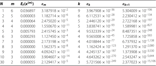
Table 1 Values ofm,k, andεkfor Example 7.1 (R= 0.125)
N m Ef(x(m)) εm k εk εk+1
[image:22.595.142.451.258.356.2]1 2 0.010032 1.457548×10⁻² 4 4.385760×10⁻²¹ 8.919073×10–63 2 1 0.067725 1.242914×10⁻¹ 3 1.347060×10–38 7.284576×10–193 3 1 0.015716 2.300541×10⁻² 3 1.825502×10–106 5.054741×10–744 4 1 0.002730 3.887455×10⁻³ 2 1.330837×10⁻²⁵ 3.543773×10–230 5 1 0.001215 1.722883×10⁻³ 2 4.720064×10–37 2.999643×10–407 6 1 0.000206 2.927439×10⁻⁴ 2 1.060096×10–50 5.523501×10–657 7 1 0.000081 1.155284×10⁻⁴ 2 6.261239×10–67 3.252761×10–1,002 8 1 0.000014 1.986052×10⁻⁵ 2 6.080606×10–85 3.570038×10–1,439 9 1 0.000005 7.910775×10⁻⁶ 2 1.309022×10–105 1.170454×10–2,002 10 1 0.000000 1.366899×10⁻⁶ 2 4.301615×10–128 8.477451×10–2,683 100 1 0.000000 1.820743×10–57 1 1.820743×10–57 3.460397×10–11,451
Table 2 Numerical results for Example 7.1 in the caseN= 10
k x1(k) x2(k)
0 0.5 + 0.5i –1.36 + 0.42i
1 1.000000380419496 + 0.000000816235730i –1.000000220051461 – 0.000000495915480i
2 1.000000000000000 + 0.000000000000000i –1.000000000000000 + 0.000000000000000i
k x1(k) x2(k)
0 –0.25 + 1.28i 0.46 – 1.37i
1 0.000000277962637 + 0.999999578393062i –0.000000314533436 – 0.999998669784542i
2 0.000000000000000 + 1.000000000000000i 0.000000000000000 – 1.000000000000000i
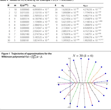
Table 3 Values ofm,k, andεkfor Example 7.2 (R= 0.043061)
N m Ef(x(m)) εm k εk εk+1
1 6 0.036897 3.187918×10⁻² 9 3.967908×10–36 5.304009×10–106 2 5 0.000003 1.182714×10⁻⁶ 6 6.112531×10⁻²⁸ 2.230412×10–134 3 4 0.000064 2.475020×10⁻⁵ 5 2.446120×10⁻²⁹ 2.722168×10–197 4 4 0.000000 1.550670×10⁻¹¹ 5 3.838741×10–93 1.589981×10–827 5 3 0.005793 2.415745×10⁻³ 4 9.532339×10⁻²⁴ 8.487351×10–248 6 3 0.000293 1.127450×10⁻⁴ 4 9.565008×10–45 1.725858×10–565 7 3 0.000005 2.173198×10⁻⁶ 4 4.018844×10–77 6.737932×10–1,138 8 3 0.000000 1.562375×10⁻⁸ 4 1.162424×10–123 1.291370×10–2,080 9 3 0.000000 4.092421×10⁻¹¹ 4 4.245137×10–187 1.373908×10–3,530 10 3 0.000000 3.904607×10⁻¹⁴ 4 4.643262×10–270 2.543247×10–5,644 30 2 0.000055 2.129417×10⁻⁵ 3 5.721566×10–249 2.377023×10–15,106
In Table , we present numerical results for Example . in the caseN= .
Example . We consider the polynomial
f(z) =z+z+
and Aberth’s initial approximationx()∈Cngiven by (see Aberth [] and Petkovićet al. []):
x()ν = – a
n +rexp(iθν), θν= π
n
ν–
,ν= , . . . ,n, (.)
[image:22.595.146.449.394.522.2]