OPTIMAL FUND ALLOCATION FROM CERTAIN INVESTMENT PORTFOLIO USING BACKWARD DYNAMIC PROGRAMMING RECURSIONS WITH ELECTRONIC IMPLEMENTATIONS

(1)

OPTIMAL FUND ALLOCATION FROM CERTAIN INVESTMENT

PORTFOLIO USING BACKWARD DYNAMIC PROGRAMMING

RECURSIONS WITH ELECTRONIC IMPLEMENTATIONS

1

Ukwu, Chukwunenye; 2Manjel, Danladi & 3Kutchin, Stephen

1,2,3Department of Mathematics, University of Jos, P.M.B 2084, Jos, Plateau State, Nigeria.

ABSTRACT

This research article investigated the problem of fund allocations from certain investment portfolio and obtained the optimal investment strategies using backward dynamic programming recursive approach. In the sequel, the article conceptualized, formulated and designed Excel solution templates and corresponding algorithm for the optimal allocation of funds from the investment portfolio. The work also provided illustrative examples which demonstrate the efficiency, utility and processing power of the solutions templates. The deployment of the solution templates circumvents the inherent tedious, and prohibitive manual computations associated with dynamic programming formulations and recursions and may be optimally appropriated for sensitivity analyses on such models.

Keywords: Dynamic programming, Optimal, Algorithm, Solution templates, Investment

portfolio, Fund Allocation.

1. INTRODUCTION

One of the challenges faced by investor’s today in search of comfortable ways to earn higher

returns on their investments above the current certificate of deposit (CD) and interest rates is the

efficient allocation of funds, which is one of the most important functions of the financial

management in modern times, Gupta and Hira [1].

Inte rnational Research Journal of Natural and Applied Sciences

ISSN: (2349-4077) Impact Factor- 5.46, Volume 4, Issue 7, July 2017 Website- www.aarf.asia, Email : [email protected] , [email protected]

(2)

The optimal investment policy has been investigated for a portfolio of two banks in a certain

class of investment problems using deterministic dynamic programming recursions Taha [2].

Unfortunately the related issue of computational feasibility is yet to be addressed. Dynamic

programming iterations are computationally intractable and doomed to failure for practical

purposes, especially for large scale applications. The need for electronic implementation of

optimal investment policies is imperative. The main contributions of this work will be as

follows: it will extend the optimal investment policy to an arbitrary number of banks. It will also

automate the computations of the optimal investment policies, thereby circumventing the

prohibitive manual computations associated with dynamic programming approach and paving

the way for sensitivity analyses on the model, the latter of which could hardly be contemplated in

manual computations.

The main purpose of this finding is to obtain the optimal policy prescriptions for fund allocation

from certain investment problems involving an arbitrary number of banks. This study will also

formulate and design corresponding Excel automated solution templates using deterministic

dynamic programming recursions. The solution templates will be motivated by the earlier works

of Ukwu [3,4,5,6] and the way these were deployed to eliminate computational tedium and other

constraints, as well as pave the way for sensitivity analyses with guarantee for instant generation

of optimal investment strategies, as soon as the pertinent data were keyed in. These activities

could hardly be contemplated in manual computations.

The template outputs of this paper will reflect and demonstrate consistency with the base results.

The findings of this study will be of great benefits to the financial sector of the economy

especially to investors and bank managers. In particular, the deployment of the solution

templates will circumvent the computational drudgery of the key indicators as well as facilitate

the sensitivity analyses on the model parameters thereby addressing the issue of

computational feasibility and timely recommendation of optional investment strategies.

2. THEORETICAL ANALYSIS

2.1 Compound Interest Computations

The Total Accumulated Value (TAV), is the principal sum plus compounded interest and is

(3)

TAV = 1

nt

i P

n



 

 

  ,

where P is the principal sum;

i

is the nominal interest rate; n is the annual compounding frequency;

t

is the planning horizon length the interest is applied.

Using the backward dynamic recursions

 

1 1

0 _,

0

( ) max { _ ( _)}, 1, 2,..., 1; _ _

  

    _n _n

i i i i i

Ii j xi

f x

f x s f x i n

the following problem of obtaining the optimal investment policies for a given portfolio of banks

with prescribed annual interest rates and end-of-year bonuses was solved in Ukwu et al [7]:

2.2 Proble m State ment

Maximize z = 1





n i

i

s





1 , , 1

s.t. , 1, 2, ... 1

k

n i i j i j j

i

s I    i n





 





, , , , , , ,

1 1 1

,

k k k

n n j n j n j n j n j n j n j

j j j

I q I I q

s  

  















where

k : Number of banks to be invested in

i

P: Fixed component of the amount for investment in all k banks at the start of year

i

, 1, 2, ... 

i n

, i j

r

: Nominal annual interest rate offered by bank jin year i ,j1, 2, ...,k

,1, ,2,... ,

i i i k

q q q : Bonus percentages paid at the end of year i in which investment is made in all k

banks.

i

x : Variable amount available for investment in all k banks in year i (includesPi)

,

i j

I : Actual amount invested in bank j at the beginning of year i

i

s : Accumulated sum at the end of year i given that I_{i j}_, is the investment made in bank jat the

beginning of yeari, j1, 2, ...,k;i1, 2, ...,n

( )

i i

(4)

 

₁

 

₁ , 1, 2, , .

i i i i i i n

s  f x  f_ x_  

The electronic computational process for the optimal investment strategies and corresponding

returns are detailed as follows:

3. RESULTS AND ANALYSIS

3.1 Excel Solution Templates and Electronic Computations for the Optimal Policy Prescriptions and Returns

3.1.1 An Algorithm for the Imple mentation of Theorem on Available and Accumulated Funds

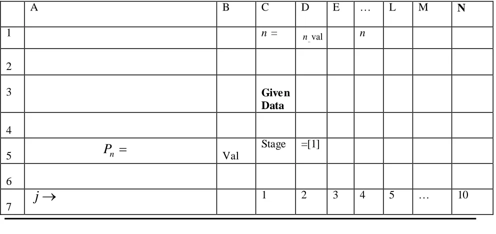
Step 1: Design of Excel Solution Te mplate

Table I: Excel Spreadsheet Layout, Documentation, Data and Fixed Value Storage, Stage Numbering, Policy Prescriptions and Reward Automation.

A B C D E … L M N

1 n = _n _val

 n

2

3 Given

Data

4

5 Val

Stage =[1]

6

7

j



1 2 3 4 5 … 10

  









 



*

min{ 1, }

max coeff. of in stage

(1 )

1 - max coeff of in

i

i j i i n i

n

i n

i n

i i x i

I x c

i

P x f x

f x x

   





 

  







n

[image:4.612.66.562.475.709.2]

(5)

8

r

n j,  rn,1 rn,2 rn,3 rn,4 rn,5 … rn,12

9



j 

=[4]

10

,

; n n j

P q  Pn

q

_n_,1

11 xn1 component coeff. _=[6]

12 xn, coeff. of In j, j qn j,

= [8]

13 _Max_coeff_{. of} _in ₍ ₎

n n

n f x x

= [9]

14 j*

= [10]

15

c

n

=[13] =[12]

16

x

n



= [11]

17 18

P

n1

Stage = [2] 19

20 j 21 rj  22



j 

=[5]

23





1,

comp.coeff.in stage 1 : ;

n

n n j

x n

P q_



24 



max coeff. of in  



comp.coeff.in stage ( 1)

n n n

n

x f x

x n

 

=[7]

25

Return func.coeff(RFC): precd. contiguous row

j

 

=[14]

26 Max coeff. of xn1in fn1



xn1



=[15] 27

*

j =[16]

28 cn1

=[17] =[20] = [19]

29 xn1

=[18]

30 31 Pn2

(6)

32

33 j 34

r

j



35 j 

36 1





1 2 ,

comp.coeff.in stage 2 : ;

n

n n j

x n

P q



 



37 



1 1 1 



1

max coeff.of in

( 2)

comp.coeff.in stage

n n n

n

x f x

n

x

  

 



38

Return func.coeff(RFC): pred.contiguous row

j

 

39 Max coeff. of xn2in fn2



xn2



40

j

*

41

c

i 42

x

i



43

44

P

n3 45

46

j



47

r

j



48



j



49 2





2 3,

comp. coeff.in stage 3 :

; n

n n j

x n

P q



 



50 _ 2 2 2  _

2

max coeff.of in

comp.coeff.in stage ( 3)

n n n

n

x f x

x n

  



 

51

Return func.coeff(RFC):

pred.contiguous row

j

 

52 xn3in fn3

 

xn3

(7)

min{ 1, } 1 1

Note that { , 1, ,1} since 0, and min{ 1, } 1,

for { 1, 2, ,1}.

(.) (.), (.)

n n n

i n i n

i n n i n i

i n n

     

     

  

 





Use Excel column A and other indicated cell references for identifiers and documentation, as

shown above. Save the nominal interest rate data in stages n n, 1,andn2, in Excel rows

   

813 ni ,i n n, 1,n2 , in contiguous cell locations, beginning from column B; save the maintenance cost data in Excel row 7, in contiguous cell locations, beginning from column C;

save the fresh money and bonus data in Excel row 10, in contiguous cell locations, beginning

from column B; save the identifiers in the remaining stages n1 to 1 in the above table, using the Copy and Paste functionality. Consecutive stages should be separated by a blank row.

Store the planning horizon length n in the fixed (absolute) cell references $D$1.

To automate the stage numbering, perform the following actions:

= [1]: Store the last stage number nunder the relative cell reference $D5.

= [2]: Secure the stage number n1under the relative cell reference $D18.

= [3]: Secure the stage number n2under the relative cell reference $D31.

Step 2: Automation of other computations in stages n n, 1, and n2.

From this step onward, horizontal crosshair dragging is associated with each code indicated by

= [integer h]: , starting from = [ 4h]:

(a) Automation of



1 _,



n

ij j

i

r_ 

 







= [4]: Type the code for _n₁, in C9, followed by the keyboard code execution <Enter>.

Click back on cell C9 and position the cursor at the right edge of the cell until a crosshair

appears. Then drag the crosshair across to the last the cell N9 to secure n j, ,j2,,k with

trailing blank spaces.

Henceforth, the act of clicking back on a specified cell, positioning the cursor at the right edge of

the cell until a crosshair appears and the crosshair-dragging routine will be referred to as clerical

(8)

= [5]: Store the code for _n__1,1

,

in C22.

Perform the horizontal clerical duty across to the last cell location N22, to secure

 

1, , 2, ,

n j j k

 _  

and trailing blanks. Now copy C22:L22 and paste it successively onto the cell references





















C 5 13 ni : L 5 13 ni , for i n2,, 2,1 ,to secure





 

,

1 , 2, ,1

n

j i

i j r i n 





    

(b)Automation of xn1 components

= [6]: Store the code for the first x_n_₁ component, in B11. Then perform the horizontal clerical

duty across to the last cell location L11 to secure the remaining components and trailing blanks.

= [7]: Store the codeto securethe first value of

 

max coeff. of x_n in f_n x_n 



x_n comp. coeff.in stage (n1)



, in B24.

Then perform the horizontal clerical duty across to the last cell location L24 to secure the

remaining values and trailing blanks. Copy the operation in [7] to B37:L37 in stage (n2).

(c) Automation of stage noutputs:_{n j}_, q_{n j}_, , Max coeff ofx_n in f x_n( _n), *,j x_n,f x_n( _n),s_n:

=[8]:Store the code for _n_,1 q_n_,1

,

in C12; then perform the horizontal clerical duty across to the

last cell location L12, to obtain n j, qn j, ,j2,,kand trailing blanks.

= [9] Storethe codefor the maximum coefficient of x_n in (f_n x_n), in [C13:L13].

= [10] Store the code for the arg max, j* of (f_n x_n), in [C14: L14].

= [11]: Store the code for the available fund, x_n,for investment at the beginning of yearn, in

[C16:L16].

= [12] Store the code for f x_n( _n), in N15.

= [13] Store the code for s_n

,

in M15.

(d) Automation of Return Function Coefficients in stage(n1):

 

   

1, max coeff. of in n comp. coeff.in stage ( 1) .

n j xn fn xn x n

 _   

(9)

 





1,0

1,0 max coeff. of in comp. coeff.in stage ( 1) ; 0,

_n_  x_n f_n x_n  x_n n _n_ 

in B25; then perform the horizontal clerical duty across to the last cell location L25 to obtain

 









1, max coeff. of n in n n n comp. coeff.in stage ( 1) ; 1, ,

n j x f x x n j k

 _      and trailing blanks.

Automation of Max coeff. of

 

1 1

1in n n

n f x

x_ _ _

=[15]:Store the code for Max coeff. of

 

1 1

1in n n ,

n f x

x_ _ _ in[C26:L26].

Automation of arg max, j*in stage n1

=[16]:Store the code for j*,in [C27:L27].

Automation of c_n_₁

=[17]:Store the code for c_n_₁

,in B28.

Automation of x_n_₁

=[18]:Store the code for x_n_₁

,

in [C29:L29].

Automation of f_n_₁(x_n_₁)

=[19]:Store the code for ₁( ₁),

n n

f _ x _ in N28.

Automation of s_n_₁

=[20]:Store the code for s_n_₁

,

in M28

Step 3: Automation of other computations in stages n2,n3,,1

(a) Copy the contiguous region $A18:N29 of stage n1 into the contiguous region $A31:N42 of stage n– 2; Modify the code in D31 to ‘=$D18-1’ to secure stage (n– 2) computational values

 

(b) Stage Implementations, i i {n 3,, 2, 1}, in One Fell Swoop

This is a crucial step involving a single Copy and n3 Paste Operations, using the

contiguous region

$A31:N42 of stage(n2).Simply use the Copy and Paste functionality to copy and paste the

(10)

Note: Consecutive stages should be separated by a blank row. In other words, for

{ 3, 4, ,1}

i n n  the Copy and Paste functionality can be used to copy and paste the

contiguous region $A31:L42 successively into stages (n3) to 1regions:

















A$ 5 13 ni : N$ 16 13 ni .

3.2 Remarks on the Use of the Templates for Large Problem Sizes

It is clear that the crosshair horizontal-dragging routine must be extended beyond column N,

as appropriate, if k11.This can be optimally done before the Copy and Paste operations from stagen1._{Hence the template can be adequately appropriated for sensitivity analyses on this}

class of Investment problems in just a matter of minutes, as contrasted with manual

investigations that would at best consume hours or days with increasing values of k and/orn, not

to talk of the dire consequences of committing just one error in any stage computations.

The template can now be deployed to obtain the optimal investment strategies and corresponding

returns, for a portfolio of nine banks, with a horizon length of eight years:

3.3 Proble m 1: 9–Bank- 8 - Year Horizon-Length Proble m

Given the amount $5, 000,000 to be invested now and $3, 000,000, $7, 000,000, $5,

000,000, $2,000,000, $10, 000,000, $8, 000,000 and$13, 000,000 at the start of years 2, 3, 4, 5,

6, 7, and 8. The annual interest rates offered by bank 1 for years 1, 2, 3, 4, 5, 6, 7, and 8 are given

by 1.3%, 0.8%, 2.1%, 0.7%, 1.65%, 2.11%, 0.75% and 1.27% compounded annually, and the

bonuses over the next 8 years are 0.25%, 0.9%, 1.66%, 1.7%, 1.55%, 0.74%, 2.2% and 1.48%

respectively. The annual interest rates offered by bank 2 are 0.4%, 0.1%, 0.3%, 1.7%, 1.22%,

0.99%, 1.32%, and 1.47% and the bonuses over the next 8 years are 1.14%, 1.2%, 1.3%, 1.25%,

1.65%, 1.29%, 2%, 1.72% respectively. The annual interest rate s offered by bank 3 are lower by

0.2% than that of bank 1 but its bonuses are higher by 0.4%.

The annual interest rates offered by bank 4 are 2.6%, 2.63%, 1.72%, 1.37%, 1.8%, 2.5%, 1.48%,

1.56% and the bonuses are 0.7%, 1.52%, 1.7%, 2.6%, 0.9%, 0.7%, 0.83% and 1.58%

respectively.

The annual interest rates offered by bank 5 are higher by 0.3% than that of bank 2, but its

(11)

The annual interest rates offered by bank 6 are 1.27%, 2%, 1%, 1.5%, 1.23%, 1.72%, 0.6%,

1.2% and its bonuses are 2.1%, 1.3%, 0.2%, 0.1%, 0.72%, 0.75%, 1.7% and 2.6%.

The annual interest rates offered by bank 7 are lower by 0.5% than that of bank 4 but its bonuses

are higher by 0.08%.

The annual interest rates offered by bank8 are 2.16%, 2.1%, 2.6%, 1.92%, 1.11%, 1.3%, 1.52%,

1.6% and the bonuses are 1.68%, 1.8%, 1.62%, 1.23%, 1.1%, 1.73%, 0.7%, and 2.4%

respectively.

The annual interest rates offered by bank 9 are lower by 0.3% than that of bank 6 but its bonuses

are higher by 0.27%. The objective is to maximize the accumulated capital at the end of 8 years.

Table 2: Pertinent Data for Proble m 3.3, with Legend

1

2

3

4

5

6

7

8

9

1

2

3

4

5

6

7

8

9

Year

P

1

5000000 0.01300 0.00400 0.01297 0.02600 0.00401 0.01270 0.02587 0.02160 0.01266 0.00250 0.01140 0.00251 0.00700 0.01137 0.02100 0.00701 0.01680 0.02106

2

3000000 0.00800 0.00100 0.00798 0.02630 0.00100 0.02000 0.02617 0.02100 0.01994 0.00900 0.01200 0.00904 0.01520 0.01197 0.01300 0.01521 0.01800 0.01304

3

7000000 0.02100 0.00300 0.02096 0.01720 0.00301 0.01000 0.01711 0.02600 0.00997 0.01660 0.01300 0.01667 0.01700 0.01297 0.00200 0.01701 0.01620 0.00201

4

5000000 0.00700 0.01700 0.00699 0.01370 0.01705 0.01500 0.01363 0.01920 0.01496 0.01700 0.01250 0.01707 0.02600 0.01247 0.00100 0.02602 0.01230 0.00100

5

2000000 0.01650 0.01220 0.01647 0.01800 0.01224 0.01230 0.01791 0.01110 0.01226 0.01550 0.01650 0.01556 0.02630 0.01646 0.00720 0.02632 0.01110 0.00722

6

10000000 0.02110 0.00990 0.02106 0.02500 0.00993 0.01720 0.02488 0.01300 0.01715 0.00740 0.01290 0.00743 0.01720 0.01287 0.00750 0.01721 0.01730 0.00752

7

8000000 0.00750 0.01320 0.00749 0.01480 0.01324 0.00600 0.01473 0.01520 0.00598 0.02200 0.02000 0.02209 0.00600 0.01995 0.01700 0.00600 0.00700 0.01705

8

13000000 0.01270 0.01470 0.01267 0.01560 0.01474 0.01200 0.01552 0.01600 0.01196 0.01480 0.01720 0.01486 0.01200 0.01716 0.02600 0.01201 0.02400 0.02607

=

0.9980

=

1.0040

=

1.0030

=

0.9975

=

0.9950

=

1.0008

=

0.9970

=

1.0027

Bank

Nominal Annual Interest Rates

End-of-Year Bonuses

Bonus Relations

Interest Relations

i

r

₃

r

_i₁

i

r

₅

r

_i₂

i

r

₇

i

r

₉

r

_ii₆

r

₄

i

q

₃

q

_i₁

i

q

₅

q

i2

i

q

₇

q

_i₄

i

q

₉

q

_i₆

{ , , , }

(12)

Table 3: Te mplate Outputs for Optimal Policies and Returns: Stages 8 to 5

n = 8 k = 9

13000000Stage 8

1 2 3 4 5 6 7 8 9

0.01270 0.01470 0.01267 0.01560 0.01474 0.01200 0.01552 0.01600 0.01196 1.0127 1.0147 1.0126746 1.0156 1.014744 1.012 1.01552 1.016 1.01196 13000000 0.01480 0.01720 0.01486 0.01200 0.01716 0.02600 0.01201 0.02400 0.02607

0 0 0 0 0 0 0 0 0 0

1.0275 1.0319 1.0275338 1.0276 1.031901 1.038 1.02753 1.04 1.03803 1.04

8

13689572.68 13689572.68 13163051

8000000 Stage 7 Computations

1 2 3 4 5 6 7 8 9

0.00750 0.01320 0.00749 0.01480 0.01324 0.00600 0.01473 0.01520 0.00598

1.0203 1.028094 1.020254469 1.030631 1.028179 1.01807 1.03048 1.03144 1.01802

8000000 0.02200 0.02000 0.02209 0.00600 0.01995 0.01700 0.00600 0.00700 0.01705

8320000 0.02288 0.0208 0.02297152 0.00624 0.020748 0.01768 0.00624 0.00728 0.01773 8320000 1.04318 1.048894 1.043225989 1.036871 1.048927 1.03575 1.03672 1.03872 1.03575

1.048927 5

13520000 8403270.15 22092842.82

8172965

10000000Stage 6 Computations

1 2 3 4 5 6 7 8 9

0.02110 0.00990 0.02106 0.02500 0.00993 0.01720 0.02488 0.01300 0.01715

1.04182 1.038272 1.041738784 1.056397 1.038388 1.03558 1.05611 1.04485 1.03547

100000000.00740 0.01290 0.00743 0.01720 0.01287 0.00750 0.01721 0.01730 0.00752

10489269 0.00776 0.013531 0.007793107 0.018042 0.013497 0.00787 0.01806 0.01815 0.00789 10489269 1.04959 1.051803 1.049531891 1.074438 1.051886 1.04345 1.07417 1.063 1.04336

1.074438 4

21911415 10623231.3 32716074.15

10056101

1 2 3 4 5 6 7 8 9

0.01650 0.01220 0.01647 0.01800 0.01224 0.01230 0.01791 0.01110 0.01226

1.05901 1.050939 1.058893097 1.075412 1.051095 1.04832 1.07502 1.05645 1.04817

2000000 0.01550 0.01650 0.01556 0.02630 0.01646 0.00720 0.02632 0.01110 0.00722

2148876 0.01665 0.017728 0.016720407 0.028258 0.017684 0.00774 0.02828 0.01193 0.00776 2148876 1.07567 1.068667 1.075613504 1.10367 1.068779 1.05606 1.1033 1.06838 1.05593

1.10367 4

32655797 2293976.37 35010050.52

2133114 j

j

r 

Coeff of

, n j j n j n I q

x  

* j

Max coeff of in ( )xn f xn n

j r  j   j r  * j

2 2 2

Max coeff of xn in fn(xn)

j

r 

j

 

j

1 1 1

Max coeff of x_n_ in f_n_(x_n_) * j * j j * j j   j r  j   RFC Coeff of In j j qn j

* j

3 3 3

Max coeff of xn in fn(xn) j * j* j j  

2 component coeff. x

j

 

1 component coeff. 

n

x

Max coeff. of in ( ) * comp. coeff. in stage 1x f x_n _{n n} x_n n Return function coeff (RFC): precd. contiguous row

j

 



Max coeff. of in ( ) * comp. coeff. in stage 2x f xn1 n n 1 1

 

xn1 n



Return function coeff (RFC): precd contiguous row

j

 

1

n p_

n p 

; ,

n n j

p q 

1,

comp. coeff. in stage ( 1) : ; 

n n n j

x n p q

 ( ) i i f x         * 1 (1 )

1- max coeff of in ( i j i i n i

i i i i

n i n

i

I x c

f x x i x

P_ x_ f_x_

           i c i c i

c

i x  i x  i c i x  2 n p 

1 comp. coeff. in stage ( 2) : 1, 2,

n n n j

x_ n P_ q_

i

x 

, if 1

i i xP i

3 n

P_

3, 3, n n j

P_ q_

i

(13)

[image:13.612.75.543.45.654.2]

Table 4: Te mplate Outputs for Optima l Policies and Returns: Stages 4 to 1

1 2 3 4 5 6 7 8 9

0.00700 0.01700 0.00699 0.01370 0.01705 0.01500 0.01363 0.01920 0.01496

1.06643 1.068805 1.066290524 1.090145 1.069017 1.06405 1.08968 1.07673 1.06385

5000000 0.01700 0.01250 0.01707 0.02600 0.01247 0.00100 0.02602 0.01230 0.00100

5518348 0.01876 0.013796 0.018837431 0.028695 0.013761 0.0011 0.02872 0.01358 0.00111 5518348 1.08519 1.082601 1.085127955 1.11884 1.082778 1.06515 1.1184 1.09031 1.06496

1.11884 4

34863136 5581306.85 40591357.38

5119784 7000000 Stage 3 Computations

1 2 3 4 5 6 7 8 9

0.02100 0.00300 0.02096 0.01720 0.00301 0.01000 0.01711 0.02600 0.00997

1.08882 1.072011 1.08863784 1.108895 1.072234 1.07469 1.10833 1.10473 1.07446

7000000 0.01660 0.01300 0.01667 0.01700 0.01297 0.00200 0.01701 0.01620 0.00201

7831882 0.01857 0.014545 0.018647041 0.01902 0.014509 0.00224 0.01904 0.01813 0.00224 7831882 1.10739 1.086556 1.107284881 1.127916 1.086742 1.07692 1.12736 1.12285 1.0767

1.127916 4

40457338 7813423.55 48404780.92

1 2 3 4 5 6 7 8 9

0.00800 0.00100 0.00798 0.02630 0.00100 0.02000 0.02617 0.02100 0.01994

1.09753 1.073083 1.097329525 1.138059 1.073309 1.09618 1.13733 1.12793 1.09588

3000000 0.00900 0.01200 0.00904 0.01520 0.01197 0.01300 0.01521 0.01800 0.01304

3383747 0.01015 0.013535 0.010191846 0.017144 0.013501 0.01466 0.01716 0.0203 0.0147 3383747 1.10768 1.086618 1.107521371 1.155204 1.08681 1.11084 1.15449 1.14823 1.11058

1.155204 4

48352748 3454010.21 51858791.13

1 2 3 4 5 6 7 8 9

0.01300 0.00400 0.01297 0.02600 0.00401 0.01270 0.02587 0.02160 0.01266

1.1118 1.077376 1.111566278 1.167649 1.077615 1.1101 1.16675 1.15229 1.10976

5000000 0.00250 0.01140 0.00251 0.00700 0.01137 0.02100 0.00701 0.01680 0.02106

5776018 0.00289 0.013169 0.002899561 0.008086 0.013136 0.02426 0.00809 0.01941 0.02432 5776018 1.11469 1.090545 1.11446584 1.175735 1.090752 1.13436 1.17485 1.1717 1.13408

1.175735 4

51818359 5838244.6 $57,697,036

5000000

j r

j

rj_j

 

RFC

Coeff of In j jqn j

* j

4 4 4

Max coeff of xn in fn(xn)

j * j* j j  

j r

j

rj_j

 

RFC

* j

5 5 5

Max coeff of xn in fn( )x

j * j* j j  

j r

j

rjj

 

RFC

* j

6 6 6

Max coeff of x_n_ in f_n_(x_n_)

j * j* j j  

j r

j

rjj

 

RFC

* j

7 7 7

Max coeff of x_n_ in f_n_(x_n_)

j * j* j j  

2 component coeff. x i x  i x  i c i

c

i x  i c i x  i c 4 n P

4, 4, n n j

P q

5

n P_

5, 5,

n n j

P q

6

n P

6, 6,

n n j

P q

7

n P

7, 7,

n n j

P q

i

(14)

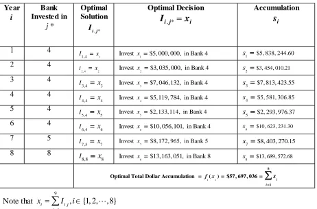
Table 5: Summary of the Optimal Investment Strategies and corresponding Returns for Proble m 3.3

Year

i

Bank Invested in

*

j

Optimal Solution

, * i j

I

Optimal Decision

, *



i j i

I

x

Accumulation

i

s

1 4

1

1,4

I x

1

Invest x $5, 000, 000, in Bank 4 s₁ $5, 838, 244.60

2 4

2 , 4 2

I  x Invest x₂ $3, 035, 000, in Bank 4 s₂ $3, 454, 010.21

3 4

3,4 3

I  x Invest x₃ $7, 046,132, in Bank 4

3 $7, 813, 423.55

s 

4 4

4,4 4

I  x Invest x₄ $5,119, 784, in Bank 4 s₄ $5, 581, 306.85

5 4

5,4 5

I  x Invest x5  $2,133,114, in Bank 4 s5 $2, 293, 976.37

6 4

6,4 6

I x Invest x₆ $10, 056,101, in Bank 4 s₆ $10, 623, 231.30

7 5

7 ,5 7

I  x Invest x7 $8,172, 965, in Bank 5 s7 $8, 403, 270.15

8 8

8,8 8

I  x Invest x₈ $13,163, 051, in Bank 8

8 $13, 689, 572.68

s 

1 1

8

1

Optimal Total Dollar Accumulation ( ) $57, 697, 036

i i

f x s



  



Note that

9

1

, {1, 2, ,8}

i i j j

x I i





 

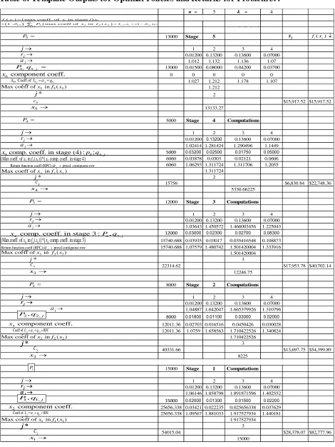
3.4 Proble m 2: Electronic Solution of the following proble m in Ukwu et al [ ]:

Given the amount $15,000 to be invested now and $ 8,000, $ 12,000, $ 5,000 and $13, 000 at the start of years 2,3 4 and 5, Table 2 furnishes the investment funds, pertinent nominal annual interest rates and end-of- year bonuses offered by a portfolio of three banks for a period of five successive years:

Table 5: Pertinent Data for Proble m 3.4

Bank Bank

1 2 3 4 1 2 3 4

Year P Nominal Annual Interest Rates End-of-Year Bonuses

1 15,000 0.012 0.0132 0.0136 0.07 0.02 0.013 0.015 0.022

2 8,000 0.012 0.0132 0.0136 0.07 0.018 0.011 0.030 0.020

3 12,000 0.012 0.0132 0.0136 0.07 0.03 0.023 0.027 0.083

4 5,000 0.012 0.0132 0.0136 0.07 0.032 0.025 0.0175 0.050

5 13,000 0.012 0.0132 0.0136 0.07 0.015 0.08 0.042 0.037

[image:14.612.68.530.73.378.2]

(15)

[image:15.612.73.543.45.671.2]

Table 6: Te mplate Outputs for Optimal Policies and Returns for Problem 3.4

n = 5 k = 4

13000 Stage 5

1 2 3 4

0.01200 0.13200 0.13600 0.07000

1.012 1.132 1.136 1.07

13000 0.01500 0.08000 0.04200 0.03700

0 0 0 0 0

1.027 1.212 1.178 1.107

1.212

2

$15,917.52 $15,917.52 13133.27

1 2 3 4

0.01200 0.13200 0.13600 0.07000 1.02414 1.281424 1.290496 1.1449

5000 0.03200 0.02500 0.01750 0.05000

6060 0.03878 0.0303 0.02121 0.0606

6060 1.06293 1.311724 1.311706 1.2055 1.311724

2

15756 $6,830.84 $22,748.36

5330.66225

1 2 3 4

0.01200 0.13200 0.13600 0.07000 1.03643 1.450572 1.466003456 1.225043

12000 0.03000 0.02300 0.02700 0.08300

15740.688 0.03935 0.03017 0.035416548 0.108873 15740.688 1.07579 1.480742 1.501420004 1.333916

1.501420004 3

22314.62 $17,953.78 $40,702.14

12246.75

1 2 3 4

0.01200 0.13200 0.13600 0.07000 1.04887 1.642047 1.665379926 1.310796

8000 0.01800 0.01100 0.03000 0.02000

12011.36 0.02703 0.016516 0.0450426 0.030028 12011.36 1.0759 1.658563 1.710422526 1.340824

1.710422526 3

40331.66 $13,697.75 $54,399.89

8225

1 2 3 4

0.01200 0.13200 0.13600 0.07000 1.06146 1.858798 1.891871596 1.402552

15000 0.02000 0.01300 0.01500 0.02200

25656.338 0.03421 0.022235 0.025656338 0.037629 25656.338 1.09567 1.881033 1.917527934 1.440181

1.917527934 3

54015.04 $28,378.07 $82,777.96

15000 j j r  5 5

5, Coeff of Ij j qj

x 

*

j

5 5 5

Max coeff of x in f (x )

j r  j   j r  * j

3 3 3

Max coeff of x in f(x)

j

r 

j

 

j

4 4 4

* j * j j * j j   j r 

2 2 RFC

Coeff of Ij j qj

*

j

2 2 2

j

* j* j

3 component coeff.

x

j

 

6 component coeff.

x

Max coeff. of in ( ) *x5 f x5 5 x5 comp. coeff. in stage 4

Return function coeff (RFC):_jprecd. contiguous row

Max coeff. of in ( ) * comp. coeff. in stage 3x4 f x4 4 x4 

Return function coeff (RFC):_jprecd contiguous row

4

P 

5

P 

5; 5,j

P q 

5comp. coeff. in stage (4) : 5; 4,j

x p q

( ) i i f x         * 1 (1 )

1 - max coeff of in ( i j i i n i

i i i i

n i n

i

I x c

f x x i x

P x f x

           5 c 3 c 2 c 5 x  4 x  4 c 3 x  3 P 

4 comp. coeff. in stage 3 : 4, 3,j

x P q

2 x 

, if 1

i i

x P i

2, 2,j

P q

j

r 

j

rjj

 

1 1 RFC

Coeff of Ij j qj

*

j

1 1 1

Max coeff of x in f(x)

j * j* j j  

2 component coeff.

x 1 c 1 x  1 P

1, 1,j

P q

i

s

2

(16)

The outputs automatically generated, following the keying in of pertinent data are consistent with

the manual solutions in [7].

4. CONCLUSION

This article designed and automated prototypical solution templates for optimal policy

prescriptions for a certain dynamic class of investment problems, with an arbitrary set of

pertinent data, complete with an algorithmic exposition on the interface and solution process.

The optimality results were realized through the interrogation of the layout of the set of feasible

data and spreadsheet locations for the various outputs at each stage, a robust investigation of the

solution templates in Ukwu [8] for the optimal investment strategies and rewards for a certain

dynamic class of probabilistic investment problemswith specified market conditions and the

transformation of the current backward dynamic recursions to special functional forms suitable

for automation on Excel platform. In the sequel, the article deployed the templates to secure the

optimal fund allocations with respect to two illustrative problems of different investment

portfolio cardinalities, demonstrating the efficiency, power and utility of the templates and their

suitability for sensitivity analyses of the problem parameters. Financial practitioners, consultants

and decision makers can leverage on these templates to enhance their confidence and portfolio of

competencies, as well as secure large market share and optimal returns on their investments.

References

[1] Gupta, P.K. & Hira, D.S. (2012). Problems in operations research (Principles and

Solutions). S. Chand & Company Ltd. New Delhi. 2012; 844-854.

[2] Taha, H.A. (2006). Operations Research: An Introduction. Seventh Edition. Prentice-Hall

of India, New Delhi. 418-421.

[3] Ukwu C. (2016). Alternative Layout and Automation of Optimality Results for Machine Replacement Problems Based On Stationary Data and Age Transition Perspectives.

Advances in Research. 7(1): 1-13.

[4] Ukwu C. (2016). Design and Full Automation of Excel Solution Templates for a

Time-perspective Class of Machine Replacement Problems with Pertinent Dynamic Data.

(17)

[5] Ukwu C. (2016). Starting Age Zero-Based Excel Automation of Optimal Policy

Prescriptions and Returns for Machine Replacement Problems with Stationary Data and

Age Transition Perspectives. Journal of Scientific Research & Reports 10 (7): 1-11.

[6] Ukwu C. (2016). An Algorithm for Global Optimal Strategies and Returns in One Fell

Swoop, for a Class of Stationary Equipment Replacement Problems with Age Transition

Perspectives, Based on Nonzero Starting Ages. Advances in Research. 7(4):1-20.

[7] Ukwu C., Manjel, D. & Kutchin S. (2017). Optimal Fund Allocation from Certain

Investment Portfolio Using Backward Dynamic Programming Recursions. International Research Journal of Natural and Applied Sciences (to appear) July 2017 Issue.

[8] Ukwu, C. (2016). Optimal investment strategy for a certain class of probabilistic investment

www.aarf.asia