AUTOMATION OF OPTIMAL PRODUCTION SCHEDULES FOR A CERTAIN CLASS OF DETERMINISTIC INVENTORY PROBLEMS USING DYNAMIC PROGRAMMING

(1)

© Associationof Academic Researchers and Faculties (AARF)

A Monthly Double-Blind Peer Reviewed Refereed Open Access International e-Journal - Included in the International Serial Directories.

Page | 1 AUTOMATION OF OPTIMAL PRODUCTION SCHEDULES FOR A CERTAIN

CLASS

OF DETERMINISTIC INVENTORY PROBLEMS USING DYNAMIC PROGRAMMING

1

Ukwu, Chukwunenye&2 Tanko, Ishaya

1

Department of Mathematics, University of Jos, P.M.B 2084, Jos, Plateau State, Nigeria. 2

Department of Computer Science, University of Jos, P.M.B 2084, Jos, Plateau State, Nigeria. ABSTRACT

This research article conceptualized, formulated and designed Excel solution templates and

corresponding exposition for optimal production schedules for a certain class of deterministic

inventory problems. The article also provided illustrative examples which demonstrated the

efficiency, utility and processing power of the solution templates. The deployment of the

solution templates circumvents the inherent tedious, and prohibitive manual computations

associated with dynamic programming formulations and recursions and may be optimally

appropriated for sensitivity analyses on each model.

Keywords: Automation, Deterministic, Dynamic programming recursions, Excel, Inventory,

Optimal production schedules, Solution Templates.

1. INTRODUCTION

The need for automation of processesis imperative; this is especially so of optimal policy prescriptionsof dynamic programming-based outputs with resulting tremendous savings in time, cost and energy. Consequently, any desired levels of sensitivity analyses can be easily undertaken and accomplished with great rapidity; needless to say that long horizon lengths can be assigned henceforth in such problems that hitherto could hardly be contemplated due to the „curse of dimensionality‟ of dynamic programming recursions.

Ukwu [1,2] designed and implemented Excel solution templates for optimal investment strategies and the corresponding optimal rewards, for the largest class of certain probabilistic International Research Journal of Mathematics, Engineering and IT

ISSN: (2348-9766) Association of Academic Researchers and Faculties (AARF)

(2)

© Associationof Academic Researchers and Faculties (AARF)

Page | 2 dynamic investment problems for practical and realistic consideration, using backward recursive dynamic programming. It went further to optimally deploy the templates for sensitivity analysis of the problem, in just a matter of minutes. These activities could hardly be contemplated in manual computations. The templates reflected and demonstrated consistency with the base results. In the sequel, Ukwu [3] designed and fully automated the solution templates for the determination of the optimal time replacement policies for a time perspective class of machine replacement problems with pertinent dynamic data given as functions of new machine purchase year and machine age. Ukwu [4,5] went on to design and automate prototypical solution templates for batch optimal policy prescriptions for a certain stationary class of equipment replacement problems, with any set of feasible starting ages, complete with an algorithmic exposition on the interface and solution process.

Ukwu et al. [6] investigated the problem of fund allocations from certain investment portfolio and obtained the optimal investment strategies using backward dynamic programming recursive approach. In what followed, Ukwu et al. [7] conceptualized, formulated and designed Excel solution templates and corresponding algorithm for the optimal allocation of funds from the investment portfolio. The work also provided illustrative examples which demonstrated the efficiency, utility and processing power of the solutions templates. A careful study of above works among others reveals that they can be leveraged and exploited for optimal production strategies of a certain class of inventory problems.

The optimal production schedule for a certain class of deterministic inventory problems using backward dynamic programming recursions has been investigated by Taha [8] and Winston [9], among other authors. Unfortunately the related issue of computational feasibility is yet to be addressed. Iterations in dynamic programming recursions are computationally intractable and doomed to failure for practical purposes, especially for large scale applications; thus, the need for electronic implementation of optimal production schedules cannot be overemphasized.

(3)

© Associationof Academic Researchers and Faculties (AARF)

Page | 3 optimal strategies, as soon as the pertinent data are keyed in. The optimality results will be facilitated by a robust investigation of the solution templates in the afore-mentioned works of Ukwu and others, and by sound reasoning regarding the implicit dependence of the dynamic programming recursions on stage numbers. Finally, this study will deploy the templates to obtain optimal production schedules for problem instances with specified entering inventories.

2. THEORETICAL UNDERPINNING

The production scheduling problem is the determination of what quantity to produce during each period to minimize the over-all production cost, given the following parameters:

(i) Problem horizon length

(ii) Entering (Incoming) inventory during each period (iii) Demand specifications for the various periods

(iv) Set up costs associated with positive production quantities (v) Holding (Storage) cost per period per unit inventory (vi) Capacity constraints on production/demand

(vii) Production function specification

The model for the paper is backward dynamic programming recursions for the determination of optimal production levels with respect to a stated class of deterministic inventory problems. 2.1 Notations for the model parameters:

T: Horizon length of the problem; t: Stage identifier; t



T T, 1,2,1



t

i : Entering inventory during period t;d_t: Demand during period t



, 1, , 2,1 .



The set of feasible entering inventory in stage ,

:

t T T

I t t  

h: Holding cost per unit inventory per period

 

t t

x i : Production quantity during period t, given that the entering inventory is i_t

2 3 4

0 1 2 3 4 :

( ) Production function

c x k k x k x k x k x

 

t t

(4)

© Associationof Academic Researchers and Faculties (AARF)

Page | 4 The relevant dynamic programming recursions are the following:

 

min





(



1

 

1



,



, 1, , 2,1



; 1

 

. 0



( )

 

( )



t

t t t t t t T T T T T T

t I

f i c x i f_ i_ t T T f _ f x i c x i

        

 

1 1 1

demand must be satisfied; production must be at nonnegative levels

there is no production activity

here must

( ) 0 ( ) 0

, ( ) , , , , , 0 .

t

;

t t t t t t t

T

t t t t t t t t t

t T

t t

d

i i x i x i

i x i d d h T f i f i

d                      



N N N R N R

N

 





0 4

 

1

be at least one positive demand during the horizon, otherwise there is nothing to solve.

j

t t j t t

j

c x i k k x i



_  _







The development of appropriate solution templatesisdetailed below and it is based on the above backward dynamic programming model.

3. METHODS, RESULTS AND DISCUSSION

3.1 Excel Implementation Template Design and interface For Optimal Production Schedules

Terminal Stage, T

A B C D E F G

1 Excel Solution…

2 Recursions

3

4 No. of periods: T Max Dem = 5

5 2 3 4

0sgn( ) 1 2 3 4

( ) x

c x k k x k x k x k x

6

7 k0 k1 k2 k3 k4

8 Values of ki:

9 Demand: dT

10 Stage = [1]

11 I x(i) f(i) = c(x)

12 0 = [3] = [5v]

13 = [2v] =[4v]

…

(5)

Page | 5 19 Penultimate Stage, T–1

20 Demand: d T-1

21 Stage = [6] Computations

22 I x(i) h i x d(  ) c x( ) f i(  x d) C+D x* f (i )

23 0 = [8] =[10v] =[11v] = [12v] =[13v] = [14v]

24 = [7v] = [9v] …

31

33 1 = [8] =[10v] =[11v] = [12v] =[13v] = [14v]

34 = [7v] = [9v] …

42

4 4

2 = [8] = [10] = [ 11] = [12] = [13] =[ 14 ]

4 5

= [7v] = [9v] …

5 3

5 5

3 = [8] =[10v] =[11v] =

[12v]

=[13v] = [14v] 5

6

(6)

© Associationof Academic Researchers and Faculties (AARF)

Page | 6 …

6 4

6 6

4 = [8] =[10v] =[11v] =

[12v]

=[13v] = [14v] 6

7

= [7v] = [9v] …

7 5

7 7

5 = [8] =[10v] =[11v] =

[12v]

=[13v] = [14v] 7

8

= [7v] = [9v] …

8 9

Stage (T-2)

91 Demand d T-2

92 Stage = [15] Computations

93 i x(i) _{h i x d}₍  ₎ _{c x}_{( )} _{f i}₍  _{x d}₎ C+D _x_* f(i )

94 0 = [17] =[19v] =[20v] = [21v] =[22v] = [23v]

95 = [16v] = [18v] …

(7)

Page | 7 The tabular process continues down to stage 1. Any stage number less than one indicates infeasibility. Blank cells also indicate forbidden choices.

3.2 Exposition on the Solution Template

“= [m] “indicates code segment m to be typed in the resident cell location.

“= [mv] “with letter v fixed indicates code segment m to be typed in the resident cell location followed by vertical crosshair-dragging activity.

Multiple “= [m] “ or“= [mv] “ indicates copying activity of the code segment from the initial cell locations.

Type the titles of the template in excel rows 1 and 2 as indicated above. Type the production cost function c(x) and its parameters in the indicated cell locations. An identifier succeeded by a colon indicates desired user input subject to the imposed restrictions.

3.3 Initialization of Stage numbering:

= [1]: Type the following code segment =$B$5, in cell location C10, <Enter> to initialize the stage number at integral input value m.

3.3.1 Stage TImplementations Incoming inventory, i :

Step 1: Input the number 0 in cell location A12.

Step 2: = [2v]: Type the following code segment =IF($A12<$B$9,1+$A12,""), in cell location A13,<Enter> to secure the next feasible higher contiguous integer. Click the cursor back on A13, position the cursor at the bottom right edge of the cell until a crosshair appears. Then drag the crosshair vertically down to cell location A17, to secure all feasible values of i.

(8)

© Associationof Academic Researchers and Faculties (AARF)

Page | 8 Production Quantity, x i_T( ):

Step 1: =[3]: “=$B$9-$A12”, in B12,<Enter>

Step 2.=[4v]: “=IF($A13 ="","",$B$9-$A13)”, in B12, followed by the clerical duty, down to B17.

Minimum Costs, f_T( ), ( )i f i , for Entering Inventory

= [5v]: “=($B$8+$C$8*$B12+$D$8*$B12^2+$E$8*$B12^3+$F$8*$B12^4)*SIGN($B12)”, inC12, followed by the clerical duty, down to C17.

3.3.2 Stage (T-1) Computations. Incoming inventory, i = 0:

Step 1: Input the number 0 in cell location A22.

Step 2: = [7v]: Type the following code segment

“=IF(COUNT(A$22:A22)<$B$9+$B$19,0,"")”, in cell location A23,followed by the clerical duty down to A31.

Production Quantity, x_T_₁( )i :

Step 1: =[8]: “=MAX($B$19-$A22,0)<Enter>

Step 2. =[9v]: “=IF(OR($A23="",$B22>=$B$9+$B$19),"",1+$B22)”, in B23, followed by the clerical duty, down to B31.

Implementation of C+D

=[12v]: “ =IF(OR($C22="",$D22=""),"",$C22+$D22)”,in E22, followed by the clerical duty, down to E31.

Implementation of x*

(9)

Page | 9 Minimum Costs, f_T_₁( )i , for Entering Inventory

= [14v]: “=IF($F22="","",$E22)”, inG22, followed by the clerical duty, down to G31.

Incoming inventory, i = 1:

Step 1: Input the number 1 in cell location A33

Step 2: = [7v]: Type the following code segment

“=IF(COUNT(A$33:A33)<$B$9+$B$19,0,"")”, in cell location A34,followed by the clerical duty down to A42.

Production Quantity, x_T_₁( )i :

Step 1: =[8]: “=MAX($B$19-$A33,0)<Enter>

Step 2: = [9v]: “=IF(OR($A34="",$B33>=$B$9+$B$19),"",1+$B33)”, in B34, followed by the clerical duty, down to B42.

Implementation of h(i+x-d)+c(x)

=[10v]: “=IF(OR($A33 = "", $B33 = ""), "",0.5*($A33+$B33-$B$19)+($B$8+$C$8*$B33+$D$8*$B33^2+$E$8*$B33^3+$F$8*$B33^4)*SIGN($B33)), in C33, followed by the clerical duty, down to C42.

Implementation off (i+x-d)

=[11v]: “=IF(OR($A33 = "", $B33 = ""), "",IF($A33+MAX($B33,0)



MAX($B$19,0)=0,MAX($C$12,0),IF($A33+MAX($B33,0)



MAX($B$19,0)=5,MAX($C$17,0),"")))))))”, in D33, followed by the clerical duty, down to D42.

(10)

Page | 10 =[12v]: “=IF(OR($C33="",$D33=""),"",$C33+$D33)”,in E33, followed by the clerical duty, down to E42.

Implementation of x*

=[13v]: “=IF($E33=MIN($E$33:$E$42),$B33,"")”, in F33, followed by the clerical duty, down to F42.

Minimum Costs, f_T_₁( )i , for Entering Inventory

= [14v]: “=IF($F33="","",$E33)”, in G33, followed by the clerical duty, down to G42. Incoming inventoryi



2, 3, 4, 5



Step 1: Input the number i in cell location A(33+(i -1)*11)

Step 2: Replace the “ 33” in the code segment “ = [7v] :“ with(33+11(i-1)) 1n cell location A(1+(33+11(i-1))),followed by the clerical duty down to A(9+(1+(33+11(i-1)))).

Production Quantity, x_T_₁( )i :i



2, 3, 4, 5



Add 11(i-1) to all relative row references in steps 1 and 2 corresponding to i =1,incorporating “=[8]:” and “ =[9v]:”.

Implementation of h(i+x-d)+c(x): i



2,3, 4,5



Add 11(i-1) to all relative row references in “ =[10v]:” and the ensuing clerical duty. Implementation of f (i+x-d): i



2,3, 4,5



Add 11(i-1) to all relative row references in “ =[11v]:” and the ensuing clerical duty. Implementation of C+D: i



2,3, 4,5



Add 11(i-1) to all relative row references in “ =[12v]:” and the ensuing clerical duty.

Implementation of x*: i



2,3, 4,5



Add 11(i-1) to all relative row references in “ =[13v]:” and the ensuing clerical duty. Minimum Costs, f_T_₁( )i : i



2,3, 4,5



Add 11(i-1) to all relative row references in “ =[14v]:” and the ensuing clerical duty.

(11)

© Associationof Academic Researchers and Faculties (AARF)

Page | 11 Implementations ofi, xi,h(i+x-d)+c(x):

Add 69 to all row references of cells in stage T-1, for corresponding ivalues, excluding the $B$8:$F$8, with global scope.

Implementations of f (i+x-d):

Replace the code segment in $D22 (for i = 0, in stage T-1) with the code segment below: “ =IF(OR($A91 = "", $B91 = ""), "",IF($A91+MAX($B91,0)



MAX($B$88,0)=0,MAX($G$22:$G$31,0),IF($A91+MAX($B91,0)



MAX($B$88,0)=1,MAX($G$33:$G$42,0),IF($A91+MAX($B91,0)



MAX($B$88,0)=4,MAX($G$66:G$75,0),IF($A91+MAX($B91,0)



MAX($B$88,0)=5,MAX($G$77:$G$86,0),"")))))))”, without the quotes.

Then apply the clerical duty from the input cell $D91down to $D100.

For i



1, 2, 3, 4, 5 ,



add 11i to all relative row references corresponding to i = 0. Implementations C+D,x* and f (i):

The code segments for C+D,x* and f (i) are invariant and hence may be copy from stage T-1 down to stage 1.

Stage t,t 



T 3,



,1 .



Implementations of i, x(i),h(i+x-d)+c(x):

Add 69 (T 2 t) to all row references of cells in stage (T-2), for corresponding i values, excluding the $B$8:$F$8, with global scope, bringing the exposition to an end.

By an appeal to Ukwu[3]the optimal production strategies can be obtained in respect of sub-horizon lengths n



1 2, ,,T 1



from the same solution template using a top-down horizon

length count in which stage





; 1 2

(12)

© Associationof Academic Researchers and Faculties (AARF)

Page | 12 3.4 EXPOSITION

3.4.1 General Application problem

A company knows that the demand for its product during each of the next T months will be as follows: montht, dtunits; t



1, 2,,T



. At the beginning of each month the company must determine how many units should be produced during the current month. During a month in which any units are produced, a setup cost of $k₀ is incurred. In addition, there is a variable quartic cost function:

2 3 4

1 2 3 4

( ) , for every units produced.

c x k x k x k x k x x

At the end of each month a holding cost of $h per unit on-hand is incurred. Historical data reveal that demand for any period does not exceedD units during each month. The company

wants to determine a production schedule that will meet all demands on time and will minimize the sum of production and holding costs during the T months.

Solve the above problem with the following pertinent data:D5,T 6

(13)

© Associationof Academic Researchers and Faculties (AARF)

Page | 13 EXCEL SOLUTION TEMPLATE OUTPUTS OF OPTIMAL PRODUCTION SCHEDULE FOR

A CLASS OF INVENTORY PROBLEMS USING DYNAMIC PROGRAMMING RECURSIONS Max Horizon

Length: 6

No of periods : 6 Max Demand: 5 h : 0.75

k0 k1 k2 k3 k4

Values of k j j = 0 ,1 , … , 4 4 1 0.0015 0.00012 0.00002

Demand : 4

Stage 6

i x(i) f(i) = c(x)

0 4 8.0368 0

1 3 7.01836 0

2 2 6.00728 0

3 1 5.00164 0

4 0 0 0

Demand 2

Stage 5 Comp.

i x(i) h(i+x-d)+c(x) f (i+x-d) C+D x* f (i)

0 2 6.00728 8.0368 14.04408

0 3 7.76836 7.01836 14.78672

0 4 9.5368 6.00728 15.54408

0 5 11.315 5.00164 16.31664

0 6 13.10584 0 13.10584 6 13.1058 4

0

1 1 5.00164 8.0368 13.03844

1 2 6.75728 7.01836 13.77564

1 3 8.51836 6.00728 14.52564

1 4 10.2868 5.00164 15.28844

1 5 12.065 0 12.065 5 12.065 4

1 6 13.85584 0 13.85584

0

4

1

( ) sgn( ) _j j

j

k k x

c x x



 



1 t i_

1

t

(14)

Page | 14

2 0 0 8.0368 8.0368 0 8.0368 0

2 1 5.75164 7.01836 12.77

2 2 7.50728 6.00728 13.5146

2 3 9.26836 5.00164 14.27

2 4 11.0368 0 11.0368

2 5 12.815 0 12.815

3 0 0.75 7.01836 7.76836 0 7.76836 1

3 1 6.50164 6.00728 12.5089

3 2 8.25728 5.00164 13.2589

3 3 10.01836 0 10.0184

3 4 11.7868 0 11.7868

3 5 13.565

4 0 1.5 6.00728 7.50728 0 7.50728 2

4 1 7.25164 5.00164 12.2533

4 2 9.00728 0 9.00728

4 3 10.76836 0 10.7684

4 4 12.5368

4 5 14.315

5 0 2.25 5.00164 7.25164 0 7.25164 3

5 1 8.00164 0 8.00164

5 2 9.75728 0 9.75728

5 3 11.51836

5 4 13.2868

(15)

Page | 15

Demand 3

0 3 7.01836 13.10584 20.1242

0 4 8.7868 12.065 20.8518

0 5 10.565 8.0368 18.6018 5 18.6018 2

0 0

1 2 6.00728 13.10584 19.1131

1 3 7.76836 12.065 19.8334

1 4 9.5368 8.0368 17.5736 4 17.5736 2

1 5 11.315 7.76836 19.0834

1

2 1 5.00164 13.10584 18.1075

2 2 6.75728 12.065 18.8223

2 3 8.51836 8.0368 16.5552 3 16.5552 2

2 4 10.2868 7.76836 18.0552

2 5 12.065 7.50728 19.5723

3 0 0 13.10584 13.1058 0 13.1058 0

3 1 5.75164 12.065 17.8166

3 2 7.50728 8.0368 15.5441

3 3 9.26836 7.76836 17.0367

(16)

Page | 16

Demand 3

0 3 7.01836 13.10584 20.1242

0 4 8.7868 12.065 20.8518

0 5 10.565 8.0368 18.6018 5 18.6018 2

0 0

1 2 6.00728 13.10584 19.1131

1 3 7.76836 12.065 19.8334

1 4 9.5368 8.0368 17.5736 4 17.5736 2

1 5 11.315 7.76836 19.0834

1

2 1 5.00164 13.10584 18.1075

2 2 6.75728 12.065 18.8223

2 3 8.51836 8.0368 16.5552 3 16.5552 2

2 4 10.2868 7.76836 18.0552

2 5 12.065 7.50728 19.5723

3 0 0 13.10584 13.1058 0 13.1058 0

3 1 5.75164 12.065 17.8166

3 2 7.50728 8.0368 15.5441

3 3 9.26836 7.76836 17.0367

(17)

Page | 17

4 0 0.75 12.065 12.815 0 12.815 1

4 1 6.50164 8.0368 14.5384

4 2 8.25728 7.76836 16.0256

4 3 10.01836 7.50728 17.5256

4 4 11.7868 7.25164 19.0384

5 0 1.5 8.0368 9.5368 0 9.5368 2

5 1 7.25164 7.76836 15.02

5 2 9.00728 7.50728 16.5146

5 3 10.76836 7.25164 18.02

5 4 12.5368

Demand 1

0 1 5.00164 18.6018 23.6034

0 2 6.75728 17.5736 24.3309

0 3 8.51836 16.55516 25.0735

0 4 10.2868 13.10584 23.3926 4 23.3926 3

1 0 0 18.6018 18.6018 0 18.6018 0

1 1 5.75164 17.5736 23.3252

1 2 7.50728 16.55516 24.0624

(18)

Page | 18

2 0 0.75 17.5736 18.3236 0 18.3236 1

2 1 6.50164 16.55516 23.0568

2 2 8.25728 13.10584 21.3631

2 3 10.01836 12.815 22.8334

3 0 1.5 16.55516 18.0552 0 18.0552 2

3 1 7.25164 13.10584 20.3575

3 2 9.00728 12.815 21.8223

3 3 10.76836 9.5368 20.3052

4 0 2.25 13.10584 15.3558 0 15.3558 3

4 1 8.00164 12.815 20.8166

4 2 9.75728 9.5368 19.2941

4 3 11.51836

5 0 3 12.815 15.815 0 15.815 4

5 1 8.75164 9.5368 18.2884

5 2 10.50728

(19)

Page | 19

Demand 5

0 5 9.065 23.39264 32.4576

0 6 10.85584 18.6018 29.4576 6 29.4576 1

0 0 0 0

1 4 8.0368 23.39264 31.4294

1 5 9.815 18.6018 28.4168 5 28.4168 1

1 6 11.60584 18.3236 29.9294

1 1 1

2 4 8.7868 18.6018 27.3886 4 27.3886 1

2 5 10.565 18.3236 28.8886

2 6 12.35584

2 2 2

3 3 7.76836 18.6018 26.3702 3 26.3702 1

3 4 9.5368 18.3236 27.8604

3 5 11.315

3 6 13.10584

(20)

Page | 20

4 2 6.75728 18.6018 25.3591 2 25.3591 1

4 3 8.51836 18.3236 26.842

4 4 10.2868

4 5 12.065

4 6 13.85584 15.35584 29.2117

4

5 1 5.75164 18.6018 24.3534 1 24.3534 1

5 2 7.50728 18.3236 25.8309

5 3 9.26836

5 4 11.0368

5 5 12.815 15.35584 28.1708

5 6 14.60584

Demand 5

0 5 9.065 29.45764 38.5226 5 38.5226 0

0 6 10.85584 28.4168 39.2726

0 7 12.66268 27.3886 40.0513

0 8 14.48936 26.37016 40.8595

0 9 16.3402 25.35908 41.6993

0 10 18.22 24.35344 42.5734

0 0 0 0

1 4 8.0368 29.45764 37.4944 4 37.4944 0

1 5 9.815 28.4168 38.2318

1 6 11.60584 27.3886 38.9944

1 7 13.41268 26.37016 39.7828

1 8 15.23936 25.35908 40.5984

1 9 17.0902 24.35344 41.4436

1 10 18.97

(21)

Page | 21

2 4 8.7868 28.4168 37.2036 4 37.2036 1

2 5 10.565 27.3886 37.9536

2 6 12.35584 26.37016 38.726

2 7 14.16268 25.35908 39.5218

2 8 15.98936 24.35344 40.3428

2 9 17.8402

2 10 19.72

2 2 2

3 3 7.76836 28.4168 36.1852 3 36.1852 1

3 4 9.5368 27.3886 36.9254

3 5 11.315 26.37016 37.6852

3 6 13.10584 25.35908 38.4649

3 7 14.91268 24.35344 39.2661

3 8 16.73936

3 9 18.5902

3 10 20.47

3 3

4 2 6.75728 28.4168 35.1741 2 35.1741 1

4 3 8.51836 27.3886 35.907

4 4 10.2868 26.37016 36.657

4 5 12.065 25.35908 37.4241

4 6 13.85584 24.35344 38.2093

4 7 15.66268

4 8 17.48936

4 9 19.3402

4 10 21.22

4

5 1 5.75164 28.4168 34.1684 1 34.1684 1

5 2 7.50728 27.3886 34.8959

5 3 9.26836 26.37016 35.6385

5 4 11.0368 25.35908 36.3959

5 5 12.815 24.35344 37.1684

5 6 14.60584

5 7 16.41268

5 8 18.23936

5 9 20.0902

(22)

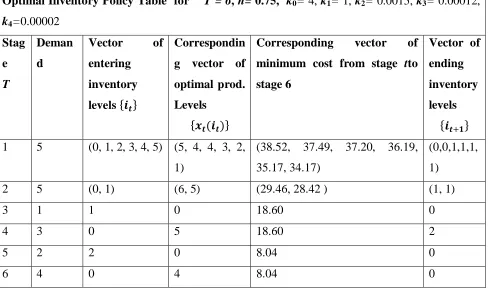
Page | 22 Using Ockham‟s razor, the optimal solutions are encapsulated in the following optimalitytable

[image:22.612.77.565.160.448.2]

Tables 1, 2 and 3: Optimal Inventory policies for specified pertinent data Table 1

Optimal Inventory Policy Table for T = 6, h= 0.75, k0= 4, k1= 1, k2= 0.0015, k3= 0.00012, k4=0.00002

Stag e

T

Deman d

Vector of entering inventory levels 𝒊_𝒕

Correspondin g vector of optimal prod. Levels

𝒙_𝒕(𝒊_𝒕)

Corresponding vector of minimum cost from stage tto stage 6

Vector of ending inventory levels

𝒊_𝒕+𝟏

1 5 (0, 1, 2, 3, 4, 5) (5, 4, 4, 3, 2, 1)

(38.52, 37.49, 37.20, 36.19, 35.17, 34.17)

(0,0,1,1,1, 1)

2 5 (0, 1) (6, 5) (29.46, 28.42 ) (1, 1)

3 1 1 0 18.60 0

4 3 0 5 18.60 2

5 2 2 0 8.04 0

6 4 0 4 8.04 0

(23)

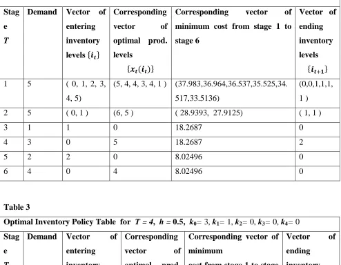
[image:23.612.74.568.124.508.2]

Page | 23 Table 2

Optimal Inventory Policy Table for T = 6, h = 0.6, k0= 4,k1= 1, k2= 0.001, k3= 0.0001, k4=

0.00001 Stag e

T

Demand Vector of entering inventory levels 𝒊_𝒕

Corresponding vector of optimal prod. levels

𝒙𝒕(𝒊𝒕)

Corresponding vector of minimum cost from stage 1 to stage 6

Vector of ending inventory levels

𝒊_𝒕+𝟏

1 5 ( 0, 1, 2, 3,

4, 5)

(5, 4, 4, 3, 4, 1 ) (37.983,36.964,36.537,35.525,34. 517,33.5136)

(0,0,1,1,1, 1 )

2 5 ( 0, 1 ) (6, 5 ) ( 28.9393, 27.9125) ( 1, 1 )

3 1 1 0 18.2687 0

4 3 0 5 18.2687 2

5 2 2 0 8.02496 0

[image:23.612.75.569.431.667.2]

6 4 0 4 8.02496 0

Table 3

Optimal Inventory Policy Table for T = 4, h = 0.5, k0= 3, k1= 1, k2= 0, k3= 0, k4= 0

Stag e

T

Demand Vector of entering inventory levels 𝒊_𝒕

Corresponding vector of optimal prod. levels

𝒙_𝒕(𝒊_𝒕)

Corresponding vector of minimum

cost from stage 1 to stage 6

Vector of ending

inventory levels

𝒊_𝒕+𝟏

1 1 ( 0, 1, 2, 3, 4, 5)

( 4, 0, 0, 0, 0, 0) ( 19.5, 16, 15.5, 15, 12.5, 12.5)

(3, 0, 1, 2, 3, 4)

2 3 ( 0, 1, 2, 3, 4) ( 5, 4, 3, 0, 0) (16, 15, 14, 11, 10.5 ) ( 2, 2, 2, 0, 1)

3 2 ( 0, 1, 2) (6, 5, 0) ( 11, 10, 7) (4, 4, 0 )

(24)

Page | 24 The solution templates act as a supervisor program for problems in the same class. In particular they reveal, as observed from the last table, the sub-optimality of Winston‟s solution, Winston [9], with respect to the entering inventory 0 in period 1,with

1(0) 20.

f 

4. SUMMARY

So far, this study has shown that manual computational process for optimal production scheduling problems is quite tedious and prone to errors. Also, it is virtually impossible to solve problems with increasing horizon length in manual computations. Electronic implementation is the only way forward for solving practical problems of reasonable sizes and the undertaking of sensitivity analyses. This is imperative for contract bidding and subsequent execution where the utility and power of the solution template can be easily demonstrated in just a matter of minutes, subject to correct data inputs and any modifications or revisions thereof.

5. CONCLUSION AND RECOMMENDATIONS

This article designed and automated prototypical solution templates for optimal policy prescriptions for a certain class of inventory problems, with an algorithmic exposition on the interface and solution process.

Consequently, relevant practical problems of any conceivable size can now be solved instantly as soon as the pertinent data have been organized and stored at the appropriate Excel cell locations, resulting in tremendous savings in time, cost and energy. Furthermore, any desired levels of sensitivity analyses can be easily undertaken and accomplished with great rapidity, needless to say that long horizon lengths can be assigned henceforth in inventory problems that hitherto could hardly be contemplated due to the „curse of dimensionality‟ .

Finally, this study deployed the templates to obtain optimal production schedules for three problems with entering inventory in the set



0,1, 2,, 5



, in just a matter of minutes.

(25)

Page | 25 implementations of optimal production policy prescriptions for the stated class of problems; thanks in particular to the breakthrough research results in Ukwu[1-5] and Ukwu et al. [6, 7].Furthermore, it is recommended that further research should be carried out on the feasibility of devising solution templates for optimal production schedules with respect to other relevant classes of inventory problems.

REFERENCES

[1] Ukwu,C. (2016). Optimal investment strategy for a certain class of probabilistic investment problems.International Research Journal of Natural andApplied Sciences. 3(2): 92-105.

[2] Ukwu,C. (2016). Sensitivity Analyses and Electronic Implementations of Optimal Investment Strategies and Rewards for a Certain Dynamic Class of Probabilistic Investment Problems.International Research Journal of Natural and Applied Sciences.3(2): 153-163.

[3] Ukwu,C. (2016). Design and Full Automation of Excel Solution Templatesfor a Time-perspective Class of Machine Replacement Problems with Pertinent Dynamic Data.Archives of Current Research International. 4(1): 1-15.

[4] Ukwu,C. (2016). An Algorithm for Global Optimal Strategies and Returnsin One Fell Swoop, for a Class of Stationary Equipment Replacement Problems with Age Transition Perspectives, Based on Nonzero Starting Ages. Advances in Research. 7(4):1-20.

[5] Ukwu,C. (2016l). Zero-Based Batch Starting Age Algorithm for GlobalOptimal Strategies and Returns, For A Class Of Stationary Equipment Replacement Problems with Age Transition Perspectives. International Journal of Advanced Research in Computer Science. 7(3): 166-186.

[6] Ukwu,C., Manjel,D. &Kutchin, S. (2017d).Optimal FundAllocation from Certain

Investment Portfolio Using Backward Dynamic Programming

(26)

Page | 26 [7] Ukwu,C., Manjel,D.&Kutchin, S. (2017c).Optimal FundAllocation from Certain Investment Portfolio Using Backward Dynamic Programming Recursions with Electronic Implementations.International Research Journal of Natural and Applied Sciences. 4(7): 283-299.

[8] Taha, H.A. (2007). “Operations Research: An introduction.”8th Edition Pearson, Prentice-Hall,New Jersey.

www.aarf.asia,