On the Nonlinear Difference Equation

http://dx.doi.org/10.4236/jamp.2016.41014

On the Nonlinear Difference Equation

Elmetwally M. Elabbasy, Abdulmuhaemn A. El-Biaty

Department of Mathematics, Faculty of Science, Mansoura University, Mansoura, Egypt

Received 17 November 2015; accepted 22 January 2016; published 26 January 2016

Copyright © 2016 by authors and Scientific Research Publishing Inc.

This work is licensed under the Creative Commons Attribution International License (CC BY).

http://creativecommons.org/licenses/by/4.0/

Abstract

In this paper, we investigate some qualitative behavior of the solutions of the difference equation

∑

n k

n k

i n i i

bx

x a n

c x

− +

− =

= + =

1

0

, 0,1, 2, , where the coefficients a, b and ci are positive real numbers,

{

}

i k, ∈ 0,1, 2, and where the initial conditions x−_k,x− +_k 1, , x0 are arbitrary positive real numbers.

Keywords

Difference Equation, Stability, Periodicity, Boundedness, Global Stability

1. Introduction

Our aim in this paper is to study with some properties of the solutions of the difference equation

1

0

, 0,1, 2, ,

n k n k

i n i i

bx

x a n

c x − +

− =

= + =

∑

(1.1)

where the coefficients ,a b and ci are positive real numbers, i k, ∈

{

0,1, 2,

}

and where the initial

condi-tions x x−k, − +k 1, , x0 are arbitrary positive real numbers. There is a class of nonlinear difference equations, known as the rational difference equations, each of which consists of the ratio of two polynomials in the se-quence terms in the same form. There has been a lot of work concerning the global asymptotics of solutions of rational difference equations [1]-[8].

Many researchers have investigated the behavior of the solution of difference equation. For example:

1

1 n .

n

n

x x

x

α −

+ = +

Our aim in this paper is to extend and generalize the work in [9], [10] and [11]. That is, we will investigate the global behavior of (1.1) including the asymptotical stability of equilibrium points, the existence of bounded so-lution, the existence of period two solution of the recursive sequence of Equation (1).

Now we recall some well-known results, which will be useful in the investigation of (1.1) and which are giv-en in [12].

Let I be an interval of real numbers and let

1

: k ,

F I + _→I where F is a continuous function. Consider the difference equation

(

)

1 , 1, , , 0,1, 2, ,

n n n n k

y+ =F y y− y− n= (1.2) with the initial condition y y−k, − +k1, , y0∈I.

Definition 1. (Equilibrium Point)

A point y I∈ is called an equilibrium point of Equation (1.2) if

(

, , , .

)

y f y y= y

That is, yn=y for n≥0, is a solution of Equation (1.2), or equivalently, y is a fixed point of f.

Definition 2. (Stability)

Let y∈

(

0,∞

)

be in equilibrium point of Equation (1.2) then

1) An equilibrium point y of Equation (1.2) is called locally stable if for every ε >0 there exists δ >0 such that, if y y−k, − +k 1, , y0∈

(

0,∞

)

with y−k− +y y− +k 1− +y + y0− <y δ, then yn− <y ε for

all n≥ −k.

2) An equilibrium point y of Equation (1.2) is called locally asymptotically stable if y is locally stable and there exists γ >0 such that, if y y−k, − +k 1, , y0∈

(

0,∞

)

with

1 0 ,

k k

y− − +y y− + − +y + y − <y γ then lim_n−∞ yn= y.

3) An equilibrium point y of Equation (1.2) is called a global attractor if for all y y−k, − +k ₁, , y₀∈

(

0,∞

)

we have

lim n .

n→∞y = y

4) An equilibrium point y of Equation (1.2) is called globally asymptotically stable if y is locally stable and a global attractor.

5) An equilibrium point y of Equation (1.2) is called unstable if y is not locally stable.

Definition 3. (Permanence)

Equation (1.2) is called permanent if there exists numbers m and M with 0< <m M < ∞ such that for any initial conditions y y−k, − +k ₁, , y₀∈

(

0,∞

)

there exists a positive integer N which depends on the initial condi-tions such that

for all .

n

m y≤ ≤M n≥ −k

Definition 4. (Periodicity)

A sequence

{ }

x_{n n k}∞₌₋ is said to be periodic with period p if xn p+ =xn for all n≥ −k. A sequence

{ }

x_{n n k}

∞ =−

is said to be periodic with prime period p if p is the smallest positive integer having this property. The linearized equation of Equation (1.2) about the equilibrium point y is defined by the equation

1

0 ,

k

n i n i

i

z+ p z− =

=

∑

(1.3)

(

, , ,

)

_{, 0,1, , .} i

n i

F y y y

p i k

y− ∂

= =

∂

The characteristic equation associated with Equation (1.3) is

1 1

0 1 1 0.

k k k

k k

p p p p

λ + λ λ − λ

−

− − −− − = (1.4)

Theorem 1.1.[13] Let

[

p q,

]

be an interval of real numbers and assume that

[ ]

1

[ ]

: , k ,

g p q + → p q

is a continuous function satisfying the following properties:

(a) g x x

(

1, , ,2 xk+1

)

is non-increasing in the first (k) terms for each xk+1 in

[

p q,

]

and non-decreasing in the last term for each xi in

[

p q,

]

for all i=1, 2, , . k

(b) If

(

m M,

)

∈

[ ] [ ]

p q, × p q, is a solution of the system

(

, , , , ,

)

and

(

, , , , ,

)

,

M g m m m= m M m g M M M= M m

implies

.

m M=

Theorem 1.2. [12] Assume that F is a _C1_{-function and let y be an equilibrium point of Equation (1.2).} Then the following statements are true:

1) If all roots of Equation (1.4) lie in the open unit disk λ <1, then he equilibrium point y is locally asymptotically stable.

2) If at least one root of Equation (1.4) has absolute value greater than one, then the equilibrium point y is unstable.

3) If all roots of Equation (1.4) have absolute value greater than one, then the equilibrium point y is a source.

Theorem 1.3. [14] Assume that p R ii∈ , =1, 2, , . k Then

1 1, k

i i= p

<

∑

is a sufficient condition for theasymptotically stable of Equation (1.5)

1 1 0, 0,1, .

n k n k k n

y+ + p y+ − ++ p y = n= _(1.5)

2. Local Stability of Equation (1.1)

In this section we investigate the local stability character of the solutions of Equation (1.1). Equation (1.1) has a unique nonzero equilibrium point

0

0 ,

.

k i i

k i i

bx x a

c x b x a

c =

=

= +

= +

∑

∑

Let

0 . k

i i

G c

=

=

∑

Then, we get

.

b x a

G

= +

(

0 1

)

0

, , , k .

k k i i i

bu f u u u a

c u =

= + ∑

(2.1)

Therefore it follows that

(

0 1

)

2

0

, , , k k j _{, 0,1, , 1,} k

j

i i i

bu c f u u u

j k u

c u =

− ∂

= = −

∂ _{ }

∑

 

 

and

(

)

1

0 1 0

2

0 , , ,

. k

i i

k i

k k

i i i

c u

f u u u _b

u

c u

−

=

= ∂

=

∂ _{ }

 

 

∑

∑

Then we see that

(

)

(

)

, ,

, 0,1, , 1, j

k

j

c

f x x _{b P j k}

uj aG b G

∂

= − = − = −

∂ +

and

(

)

(

)

, , k k _.

k k

f x x _b G c _P

u aG b G

∂ ₌ − _{= −}

∂ +

Then the linearized equation of (1.1) about x is 1

0 . k

n i n i

i

z+ p z− =

=

_∑

(2.2)

Theorem 2.1. Assume that

(

b aG G−

)

<2bck. Then the equilibrium point of Equation (1.1) is locally stable.

Proof. It is follows by Theorem (1.3) that, Equation (2.2) is locally stable if

1 0 1.

k

p ++ p + p <

That is

(

aG b Gbc0

)

(

aG b Gbc1

)

(

aG b Gbck−1

)

(

b G caG b G

(

)

k

)

1.

−

+ + + + <

+ + + +

This implies that

(

)

(

(

)

)

1

0 _1,

k i

i k

b c _{b G c}

aG b G aG b G

−

=

 

  ₋

 _{ + <}

+ +

∑

then

(

)

(

)

2

1. k

b G c aG b G

− < +

Thus

3. Periodic Solutions

In this section we investigate the periodic character of the positive solutions of Equation (1.1).

Theorem3.1. Equation (1.1) has positive prime period-two solution only if

(

)(

)

and 4 .

k odd− α β− aβ−aα+b > aαβ (3.1)

Proof. Assume that there exists a prime period-two solution , , , , ,p q p q

of (1.1). Let xn=q x, n+1= p. Since k odd− , we have xn k− = p. Thus, from Equation (1.1), we get

0 1 2

, k

bp p a

c q c p c q c p

= +

+ + ++

and

0 1 2

. k

bq q a

c p c q c p c q

= +

+ + ++

Let

0 2 k 1 ,

c +c ++c₋ =α and

1 3 k .

c c+ ++c =β Then

,

bp p a

q p

α β

= + + and

.

bq q a

p q

α β

= + + Then

2 _,

pq p a q a p bp

α +β = α + β + (3.2) and

2 _.

pq q a p a q bq

α +β = α + β + (3.3) Subtracting (3.2) from (3.3) gives

(

_p2 _q2

)

(

_{a a b p q}

)(

)

_.

β − = β − α+ −

Since p q≠ , we have

.

a a b p q β α

β

− +

+ = (3.4)

Also, since p and q are positive,

(

aβ−aα+b

)

should be positive. Again, adding (3.2) and (3.3) yields

(

2 2

)

(

)(

)

2αpq+β p +q = aα+aβ+b p q+ . (3.5) It follows by (3.4), (3.5) and the relation

(

)

2

2 2 _{2 , , R,}

p +q = p q+ − pq ∀p q∈ that

(

)

(

)

.

a a a b

pq= α β_{β α β}− α+

Assume that p and q are two distinct real roots of the quadratic equation

(

)

(

₍

₎

)

2 a a a b _0,

t a a b t α β α

β β α

α β

− +

− − + + =

−

and so

(

)

2

(

₍

₎

)

4 a a a b 0,

aβ aα b β α β α

α β

− +

− + − >

−

which is equivalent to

(

α β−

)(

aβ−aα+b

)

>4aαβ. Thus, the proof is completed.

4. Bounded Solution

Our aim in this section we investigate the boundedness of the positive solutions of Equation (1.1).

Theorem 4.1. The solutions

{ }

x_{n n k}∞₌₋ of Equation (1.1) are bounded.

Proof. Let

{ }

x_{n n k}∞₌₋ be a solution of Equation (1.1). We see from Equation (1.1) that

1

0 1 1

0

.

n k n k n k

n n k n k i n i

i

bx bx

x a a

c x c x c x c x − − + − − − = = + = + + + +

∑

Then

for all 1. n

k

b

x a M n

c

≤ + = ≥ (4.1)

On the other hand, we see that the change of variables 1 , n n x y =

transforms Equation (1.1) to the following form:

0 1

1

1

1 n k _.

k n

n n n k

b y

a c c c y

y y y − +

− −

= +

+ + +

Hence, we obtain

0

1 1

0 1

1 0, 1 0

1 _.

k n i i n k

k k k

n

n i n i k n i

i i i i

b _y y a

y _{c y c y c y} − = − − + − − − = = ≠ = = + + + +

∏

∏

∏

∏

Thus

(

)

(

)

1

0 1 0

1 0, 1 0 1

1 1 1

0 1 0 1

1 0, 1 0 1 0, 1 0

1 0, 1

0 1

1 0, 1

k k k k

n i n i k n i n i

i i i i i

n k k k k k k

n i n i k n i n i n i k n i

i i i i i i i i

k n i i i

k k

n i n i i i i

c y c y c y c y

y

ac y ac y ac b y ac y ac y ac b y

c y ac y ac y

− − − − − = = ≠ = = + − − − − − − − − = = ≠ = = = ≠ = − = ≠ − − = = ≠ + + + = = + + + + + + + + + +

∏

∏

∏

∏

∏

∏

∏

∏

∏

∏

∏

∏

(

)

(

)

1 0 1 1 0 1

0 1 0, 1 0

,

k k n i

i

k k k k

k n i n i n i k n i

i i i i i

c y

and so,

(

)

(

)

(

(

)

)

1 1 0 0, 1 1 0 1 1 0 1

1 0, 1 0

.

k

k k

n i

n i k n i

i i

i i

n k k k

n i n i k n i

i i i i

k k k

k k

c y

c y c y

y

ac y ac y ac b y k ac b ac

c k

a ac b a ac b

− − − − = ≠ = = + − − − − = = ≠ = ≤ + + + + + + = + = + +

∏

∏

∏

∏

∏

∏

(

)

(

)

1 1

1 k k_.

n

n k

k ac b ac y

x a ac b

+ +

+ +

= ≤

+

It follows that

(

)

(

)

1

1 k k _{for all 1.}

n k

k ac b ac _{E n}

x+ a ac b

+ +

≤ = ≥

+

Thus we obtain

1 1 _{for all 1.} n

n

x m n

y E

= ≥ = ≥ (4.2)

From (4.1) and (4.2) we see that

for all 1.

n

m x≤ ≤M n≥ Therefore every solution of Equation (1.1) is bounded.

5. Global Stability of Equation (1.1)

Our aim in this section we investigate the global asymptotic stability of Equation (1.1).

Theorem 5.1. If aG=2ack+b, then the equilibrium point x of Equation (1.1) is global attractor.

Proof. Let f : 0,

(

∞

)

k+1→

(

0,∞

)

be a function defined by

(

0 1

)

0

, , , k ,

k k i i i

bu f u u u a

c u =

= +

∑

then we can see that the function f u u

(

0, , ,1 uk

)

is decreasing in the rest of arguments and increasing in uk.

Suppose that

(

m M,

)

is a solution of the system

(

, , , , ,

)

and

(

, , , , ,

)

.

m f M M M= M m M = f m m m m M

Then from Equation (2.1), we see that

(

)

(

)

1 1 0 0 , , , , k k

i k i k

i i

k k k k

bm bM

m a M a

c M c m c m c M

bm bM

m a M a

G c M c m G c m c M

− − = = = + = + + + = + = + − + − +

∑

∑

(

)

(

)

(

)

(

)

2 2 , ,

k k k k

k k k k

G c Mm c m a G c M ac m bm

G c Mm c M a G c m ac M bM

− + = − + +

− + = − + +

then

(

2 2

)

(

₂

)(

)

_.

k k

c m −M = ac b aG m M+ − − Thus

.

m M=

6. Numerical Examples

For confirming the results of this section, we consider numerical examples which represent different types of solution of Equation (1.1).

Example 6.1. Consider the difference equation

1 1

1 0.9

0.5 ,

0.6 0.5n

n

n n

x x

x − x +

−

= +

+

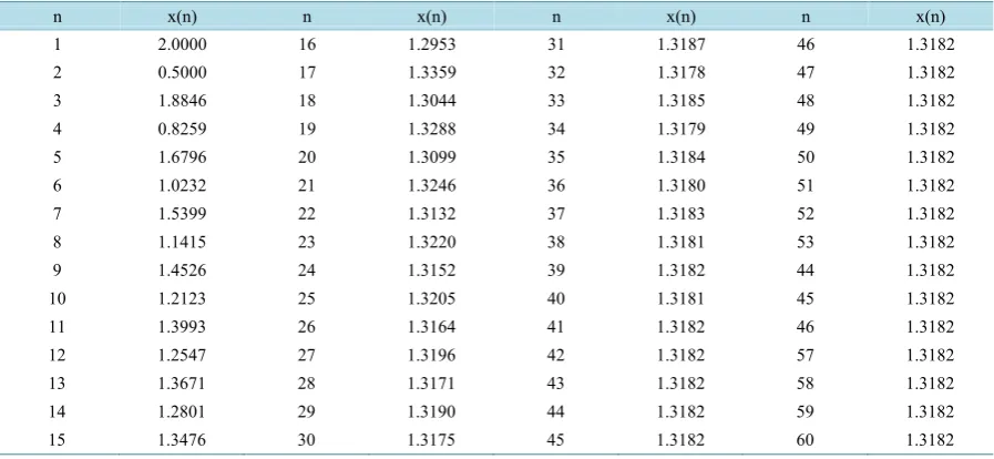
where k=1,a=0.5,b=0.9,α =c0 =0.6,β = =c1 0.5. Figure 1 shows that the equilibrium point of Equation (1.1) has locally stable, with initial data x−1=2.2,x0 =0.3 (seeTable 1).

Example 6.2. Consider the difference equation

1 1

1 4

0.125 ,

2 n

n

n n

x x

x −x +

−

= +

+

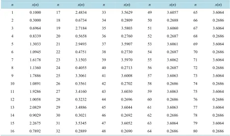
where k odd− =1,a=0.125,b=4,α =c0=2,β = =c1 1. Figure 2, shows that Equation (1.1) which is period-ic with period two. Where the initial data satisfies condition (3.1) of Theorem (3.1) x−1 =0.1,x0 =0.3 (see

[image:8.595.92.540.295.723.2]

Ta-ble 2).

Figure 1. Ref. b1.

Table 1. The equilibrium point of Equation (1.1).

n x(n) n x(n) n x(n) n x(n)

1 2.0000 16 1.2953 31 1.3187 46 1.3182

2 0.5000 17 1.3359 32 1.3178 47 1.3182

3 1.8846 18 1.3044 33 1.3185 48 1.3182

4 0.8259 19 1.3288 34 1.3179 49 1.3182

5 1.6796 20 1.3099 35 1.3184 50 1.3182

6 1.0232 21 1.3246 36 1.3180 51 1.3182

7 1.5399 22 1.3132 37 1.3183 52 1.3182

8 1.1415 23 1.3220 38 1.3181 53 1.3182

9 1.4526 24 1.3152 39 1.3182 44 1.3182

10 1.2123 25 1.3205 40 1.3181 45 1.3182

11 1.3993 26 1.3164 41 1.3182 46 1.3182

12 1.2547 27 1.3196 42 1.3182 57 1.3182

13 1.3671 28 1.3171 43 1.3182 58 1.3182

14 1.2801 29 1.3190 44 1.3182 59 1.3182

[image:8.595.90.539.513.720.2]

[image:9.595.57.538.85.363.2] [image:9.595.86.539.312.580.2]

Figure 2. Ref. b4.

Table 2. The initial data satisfies condition (3.1) of Theorem (3.1).

n x(n) n x(n) n x(n) n x(n) n x(n)

1 0.1000 17 2.4834 33 3.5629 49 3.6057 65 3.6064

2 0.3000 18 0.6734 34 0.2809 50 0.2688 66 0.2686

3 0.6964 19 2.7184 35 3.5803 51 3.6060 67 3.6064

4 0.8339 20 0.5658 36 0.2760 52 0.2687 68 0.2686

5 1.3033 21 2.9493 37 3.5907 53 3.6061 69 3.6064

6 1.0945 22 0.4751 38 0.2730 54 0.2687 70 0.2686

7 1.6178 23 3.1503 39 3.5970 55 3.6062 71 3.6064

8 1.1360 24 0.4055 40 0.2713 56 0.2687 72 0.2686

9 1.7886 25 3.3061 41 3.6008 57 3.6063 73 3.6064

10 1.0891 26 0.3561 42 0.2702 58 0.2686 74 0.2686

11 1.9286 27 3.4160 43 3.6030 59 3.6063 75 3.6064

12 1.0058 28 0.3232 44 0.2696 60 0.2686 76 0.2686

13 2.0829 29 3.4886 45 3.6044 61 3.6063 77 3.6064

14 0.9029 30 0.3021 46 0.2692 62 0.2686 78 0.2686

15 2.2675 31 3.5345 47 3.6052 63 3.6064 79 3.6064

16 0.7892 32 0.2889 48 0.2690 64 0.2686 80 0.2686

Remark 6.1. Note that the special cases of Equation (1.1) have been studied in [9] when k=1,b=1,c0 =1, 0, 1

i

c = i≥ and in [10] when k=1,b=1,c0=1,ci =0,i≥1 and in [11] when b=1,c0=1,ci=0,i≥1.

References

[1] Elabbasy, E.M., El-Metwally, H. and Elsayed, E.M. (2005) On the Periodic Nature of Some Max-Type Difference Eq-uations. International Journal of Mathematics and Mathematical Sciences, 2005, 2227-2239.

http://dx.doi.org/10.1155/IJMMS.2005.2227

[2] Elabbasy, E.M., El-Metwally, H. and Elsayed, E.M. (2006) On the Difference Equation 1

1 n

n n

n n

bx

x ax

cx dx

+

−

= −

− .

[3] Elabbasy, E.M., El-Metwally, H. and Elsayed, E.M. (2007) Qualitative Behavior of Higher Order Difference Equation.

Soochow Journal of Mathematics, 33, 861-873.

[4] El-Moneam, M.A. and Zayed, E. (2014) Dynamics of the Rational Difference Equation

1 n n k n l

n n n k n l

n k n l

bx x x

x Ax Bx Cx

dx ex

− −

+ − −

− −

= + + +

− . DCDIS Series A: Mathematical Analysis, 21, 317-331.

[5] Elaydi, S.N. (1996) An Introduction to Difference Equations, Undergraduate Texts in Mathematics. Springer, New York. http://dx.doi.org/10.1007/978-1-4757-9168-6

[6] Kocic, V.L. and Ladas, G. (1993) Global Behavior of Nonlinear Difference Equations of Higher Order with Applica-tions. Kluwer Academic Publishers, Dordrecht.

[7] Stevic, S. (2005) On the Recursive Sequence

(

)

1

1 , ,n k

n

n n k

x x

f x x

α β −

+

− +

+ =

. Taiwanese Journal of Mathematics, 9, 583-593.

[8] Zayed, E. and EI-Moneam, M.A. (2010) On the Rational Recursive Sequence 0 1 2 1

0 1 2

n n l n k

n

n n l n k

x x x

x

x B x x

α α α

β − β −

+

− −

+ +

=

+ + .

Mathema-tica Bohemica, 135, 319-363.

[9] Amleh, A.M., Grove, E.A., Georgiou, D.A. and Ladas, G. (1999) On the Recursive Sequence 1

1 n

n

n x x

x

α −

+ = + . Journal

of Mathematical Analysis and Applications, 233, 790-798. http://dx.doi.org/10.1006/jmaa.1999.6346

[10] Hamza, A.E. (2006) On the Recursive Sequence 1

1 n

n

n x x

x

α +

+ = + . Journal of Mathematical Analysis and Applications,

322, 668-674. http://dx.doi.org/10.1016/j.jmaa.2005.09.029

[11] Saleh, M. and Aloqeili, M. (2005) On the Rational Difference Equation n1 n k n x

x A

x−

+ = + . Applied Mathematics and

Computation, 171, 862-869. http://dx.doi.org/10.1016/j.amc.2005.01.094

[12] Grove, E.A. and Ladas, G. (2005) Periodicities in Nonlinear Difference Equations. Vol. 4, Chapman and Hall/CRC, Boca Raton.

[13] Elabbasy, E.M., El-Metwally, H. and Elsayed, E.M. (2007) On the Difference Equations 1

0 n k

n k

n i i x x

x

α β γ

− +

− =

=

+

∏

. Journal

of Concrete and Applicable Mathematics, 5, 101-113.