Identification of Evolving Fuzzy Rule-Based Models
Plamen Angelov, Member, IEEE, , and Richard Buswell
Abstract—An approach to identification of evolving fuzzy
rule-based (eR) models is proposed in this paper. eR models implement a method for the noniterative update of both the rule-base structure and parameters by incremental unsupervised learning. The rule-base evolves by adding more informative rules than those that previously formed the model. In addition, existing rules can be replaced with new rules based on ranking using the informative potential of the data. In this way, the rule-base struc-ture is inherited and updated when new informative data become available, rather than being completely retrained. The adaptive nature of these evolving rule-based models, in combination with the highly transparent and compact form of fuzzy rules, makes them a promising candidate for modeling and control of complex processes, competitive to neural networks. The approach has been tested on a benchmark problem and on an air-conditioning component modeling application using data from an installation serving a real building. The results illustrate the viability and efficiency of the approach. The proposed concept, however, has significantly wider implications in a number of fields, including adaptive nonlinear control, fault detection and diagnostics, performance analysis, forecasting, knowledge extraction, robotics, and behavior modeling.
Index Terms—evolving fuzzy rule-based (eR) models, fuzzy
models identification, rule-base adaptation.
I. INTRODUCTION
C
ONTROL theory (including identification and adaptive systems) has matured and is now a well-developed and structured field, its linear part in particular [2]. Real-life ap-plications, however, often do not comply with the rigorous as-sumptions under which the basic conclusions of this theory have been made. First principle models, which are based on mass and energy balances, can be difficult or even impossible to derive [3]. Many factors and time variations that influence the process are often ignored or their effects are considered a disturbance, which can result in locally applicable models. A significant por-tion of the process knowledge is qualitative and imprecise and therefore can not be used in such models [19].Fuzzy rule-based (FRB) models successfully address these is-sues, because of their inherent flexibility and transparency. Re-cently, they have been successfully used to effectively blend and interpolate different operating regimes, which could be locally linearized [4]. The main obstacle in the design of FRB models is the proper, adequate and expedient generation of their struc-ture (the rule base, membership functions and linguistic labels) and parameters. Another stumbling block, which is still unre-solved, is that fuzzy models are not adaptive. This hinders their
Manuscript received February 7, 2001; revised October 29, 2001 and March 12, 2002. This work was supported by the EPSRC under Grant GR/M27299.
The authors are with the Loughborough University, Leicestershire LE11 3TU, U.K. (e-mail: [email protected]).
Digital Object Identifier 10.1109/TFUZZ.2002.803499.
application to practical problems where the control object, or the environment, is changing significantly [9], [19].
A typical tendency until early 1990s was to rely on existing expert knowledge and to just tune fuzzy sets’ parameters using gradient-based methods or genetic algorithms (GAs) [27]. During the late 1990s, so-called data-driven or rule/knowl-edge extraction methods were intensively developed [5], [8], [10]–[12], [16]. The attempt was to identify the model structure and parameters based primarily on data. In the approach, the expert knowledge plays a nonessential role. The techniques used are mainly clustering, linear least squares and/or non-linear optimization [5], [8], [10], [16] for fine-tuning of both antecedent and consequent parts.
Very recently, in fact in parallel with this work, fuzzy neural networks [18] with evolving structure have been developed. A so-called “self-constructing fuzzy-neural network controller” [18] is primarily oriented to control applications. It uses dif-ferent mechanisms of rules/neurons update based on the error in previous steps [18], while evolving fuzzy rule-based (eR) models [9] use the informative potential of the new data sample as a trigger to update the rule-base. The latest mechanism ensures greater generality of the structural changes (that the rules are able to describe a number of data samples) from the moment of their initialization. In addition, the mechanism of rule-base modification (replacement of a less informative rule with a more informative one) is considered in [9] ensures a gradual change of the rule-base structure and inheritance of the structural information. The mechanism for rule-base structure update used in [18] tolerates the first different data samples rather than the most informative ones. It therefore makes more changes to the structure and can potentially form rules around outlays. It is not possible for an outlay to become a rule center using eR model method. In [18], the learning scheme (gradient-based error back propagation) is iterative and potentially biased to the local minimums. The consequences (output parameters) are singletons, which is simplified special case of the linear models used in [9].
eR models evolve their structure. A new rule is generated if there is significant new information present in the data collected. If the new rule is very close to an existing one the later is re-placed. This procedure is noniterative and is based on the de-scriptive potential of each data sample representing a measure of the accumulated spatial proximity of the data. The appear-ance of a new rule indicates a region of the data space that has not been covered by the initial training data. This could be a new characteristic of the process or reaction to a new disturbance. In fact, many regimes and process states can not be practically included into the training data set (such as faulty process be-havior), but states close to them could well appear during the process run.
The proposed approach distinguishes whether a new data point is an outlay by judging its informative potential. A high potential indicates that there are a number of similar data and the point is not an outlay. If the informative potential of the new data sample is high enough and it is not too close to an existing rule, it is added to the rule base without replacement of an old rule. It is important to note that learning could start without a priori information and only a few data samples. This interesting feature makes the approach potentially very useful in autonomous systems and robotics as a tool for accumulation of knowledge. Published approaches for structure adaptation, like reinforcement learning [21] and pruning [22], adapt or minimize a given, fixed structure. The proposed approach considers an evolving model structure through the inheritance, modification, and upgrade of the rule base.
Systems that are able to learn the behavior of the object of modeling and control could be considered as a basis for a third level of control [9]. The first level comprises local controllers and the second, adaptive controllers, including supervisory controllers in hierarchical systems. The distinctive element is the ability to learn (to change and enrich) their structure. Such systems could be named intelligent or smart adaptive systems [9].
Real-time online applications, however, are hampered by the need to recursive calculation of the model parameters. A com-putationally effective approach, which avoids the need of mem-orizing large matrices with the data or using of moving time windows as in [9] is treated in a future paper. Considerations in the present paper are limited to the use of all available past data. This paper is organized as follows. Fuzzy model identifica-tion is considered in Secidentifica-tion II. Identificaidentifica-tion of eR models with recursive calculation of the informative potential is presented in Section III. In separate subsections it is treated how and why the procedure works and the essential stages are defined and de-scribed. Section IV represents experimental results considering a benchmark problem of Mackey–Glass time-series predic-tion and an air-condipredic-tioning engineering component modeling problem, based on data from a real installation. Concluding remarks are given in Section V.
II. FUZZYMODELIDENTIFICATION
Fuzzy model identification has its roots in the pio-neering papers of Takagi and Sugeno [13] and Pedrycz [14]. Takagi–Sugeno (TS) fuzzy models have found much wider application than the relational fuzzy model [14], due mainly to the computational and interpretation efficiency they have
(1)
where
th fuzzy rule;
number of fuzzy rules;
input vector; ;
antecedent fuzzy sets, ;
output of the th rule;
and parameters of the consequence.
In this form, it represents multiple-input–single-output system. The degree of firing of each rule ( ) is determined by the Gaussian law, which ensures the greatest possible generalization
(2)
where
center of a rule
is a positive constant, which defines the zone of influence of the rule. Too great a value of leads to averaging, too small a value, to over-fitting. As a rule of thumb, it is recommended
to use and
to ensure smooth overlapping.
The model output is calculated by weighted averaging of indi-vidual rules’ contribution
(3)
where
diagonal matrix with its diagonal ele-ments representing the strength of the th
rule ( );
output of the th local (linear) submodel. The problem of fuzzy model identification is treated in more detail in [3], [13], and [16]. Generally, the identification of a TS model could be divided into the following two subtasks:
i) identification of the antecedent part of the model (1), which consists of determination of the centers (
) and spreads ( ) of the membership functions; ii) identification of the parameters ( and ,
, ) of the consequent
part.
The first subtask could be solved by subtractive clustering [16], which surpasses other methods, like fuzzy C-means [17], Gustafson–Kessel [23], fuzzy k-NN [24], etc. because of its simplicity and efficiency. This clustering algorithm, which is an improved version of the original mountain clustering [25], is based on the notion of the informative potential [16] of a data point ( ; where is the augmented data vector , ; denotes number of training data sam-ples). This potential depends on the spatial proximity between this point and all other data points. Instead of the Gaussian type function used in [16] and [25] we use the Cauchy form
(4)
where , denotes projection of the distance between two data points ( and ) on the axis , .
In order to solve the second subtask, to estimate the parame-ters of the consequences, first let represent the local submodels in vector form for all the training data
(5)
where
vector of parameters of the consequent part of the th rule of the TS model; matrix formed by addition of a uni-tary column to the vector in order to accommodate the role of the free coefficients .
It is interesting to note that for small increments of the inputs ( ) and the output ( ), i.e., assuming smooth mapping the parameters resembles the Jacobian of obtained by linearization of around certain data point ( ) [29].
Combining (5) with (3) in vector form for all the training data, we have
(6)
The vector of consequence parameters ( , ) could be found by linear least squares [2] applied per rule [9], [30]
(7)
where
;
or the recursive version, called the Kalman filter [2], [13], [16]
(7a)
where
weighted inputs matrix for the th rule; big number;
identity matrix; covariance matrix.
It should be noted that (7) could lead to numerical problems if matrix is singular or close to singular. is positive definite because of (2)–(3), but for distant points it could have very small values. An accepted way to overcome such numerical problems is to use pseudo-inversion [16], [28].
III. IDENTIFICATION OF ER MODELS
In this paper, a procedure for data-driven identification of eR models is considered. This allows incremental learning of both structure and parameters of the gradually evolving model as op-posed to the fixed structure models considered in the previous section. It includes the following stages.
Stage 1: Initialization of the rule-base structure (antecedent part of the rules).
Stage 2: Estimation of the parameters of the consequent part by linear least squares.
Stage 3: Prediction of the output by the eR model. Stage 4: Reading of the next data sample at the next time step.
Stage 5: Recursive calculation of the potential of each new data sample to influence the structure of the rule-base. Stage 6: Recursive up-date of the potentials of old centers taking into account the influence of the new data sample. Stage 7: The new data sample competes with the existing rules’ centers. Decision to modify or innovate the rule-base structure is taken.
The execution of the algorithm continues with Stage 2.
A. Proposed Algorithm: How it Works
Stage 1. The rule-base could contain one single rule only
based, for example, on the first few ( ) data samples. Then
(8)
where
index of the data;
number of data available initially; first rule center.
In principle, the rule-base could be initialized by existing expert knowledge. Generally, however, it could be based on the iden-tification approaches, described in the previous section. In this case
(8a)
where denotes the initial number of rules.
Stage 2. Parameters of the consequent part are determined by
least squares technique [2].
a) For the case when a new rule is added or a rule is replaced (see Stage 7), all previous data are used and parameters are cal-culated by (7). This requires the use of matrices ( and ) with increasing dimensions, which hampers direct real-time applica-tion in online mode. This problem could be overcome by in-troduction of a time moving window [9] or by using recursive least squares. It should also be noted that only a small number of data (usually about 5% as the experimental results show) has high enough potential to modify the rule base and so changes to the rule base do not occur often.
b) The structure of the model is not changed. Then, parame-ters of the consequent are determined recursively by [9]
(9)
where the first equation shown at the bottom of the next page holds.
update of the co-variation matrices and from the previous step’s calculation speeding up the algorithm execution.
At Stage 3, the output for the next time step ( ) is esti-mated using (6) as
(10)
where is the estimation (prognosis) of the output by the eR model.
At Stage 4, the next data sample is collected.
At Stage 5, the potential of each new data sample is re-cursively calculated. Transforming (4) the potential could be expressed for the first data available as
(11) or as in shown in (11a) at the bottom of the page. Substituting
the recursive expression follows:
(12)
Analyzing, it is easy to see that ( ) and could be memorized from calculations of the previous step ( ), while depends on the new data point only.
At Stage 6, the potentials of the centers of the existing clus-ters/rules are recursively updated by an amount governed by the spatial proximity between the new data point and each of them:
(13)
where denotes the potential of the th center for the th data.
The use of already calculated potentials of clusters, leads to significant time and calculation savings because these values are calculated from large matrices ( will usually be a large number). At the same time, they have accumulated information regarding the spatial proximity of all previous data.
Stage 7 compares the potential of the new data sample to
the potential of existing centers and takes decision whether to modify or innovate the rule-base.
IF the potential of the new data point is higher than certain
threshold AND the new data point is close to an old center
(14)
(14)
where
new data sample; center of the th rule; potential of the new data; potential of the th rule.
THEN the new data point ( ) replaces this old center for
(15) This mechanism (Fig. 1) is called modification of the rule base [9].
ELSE IF the potential of the new data point is higher than
certain threshold
THEN it is accepted as a new rule’s center
(16)
This mechanism is termed rule-base innovation [9]. The preservation of rules and gradual upgrade by one rule only instead of completely rebuilding the model when signifi-cant new information is available provides an inheritance of the useful information contained in rule-base structure. It should be noted that outlying data are automatically rejected because their potential is significantly lower due to their distance from the other data.
The algorithm continues with Step 2 until . In this paper, as in [9] and [16], the values of the thresholds are determined as
(17)
The upper threshold ensures that data samples with potential above the half of the best are accepted only. Its value influences the number of rules present in the final model. The value of 50% of the maximal potential showed a good balance between the model complexity and precision [9], [16] on a number of examples. The lower one defines a gray zone [16] where the data are checked on the proximity to the existing centers. It influences the number of replacements of centers, which will take place. Alternatively, both thresholds could be equal to the mean potential of all rules
(18)
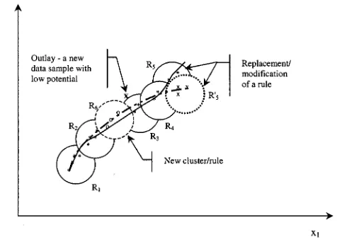
A graphical representation of the algorithm that realizes the proposed approach is demonstrated in Fig. 2. All steps are noniterative. Using the approach, a transparent compact and accurate model can be found by rule-base evolution based on experimental data with the simultaneous estimation of the fuzzy set parameters. It is interesting to note, that the upgrade rate with new rules does not lead to an excessively large rule base. The reason for this is that the proximity of a candidate center to already existing centers is controlled by a hard restriction, differing from [18] that employs pruning.
B. Proposed Algorithm: Why it Works
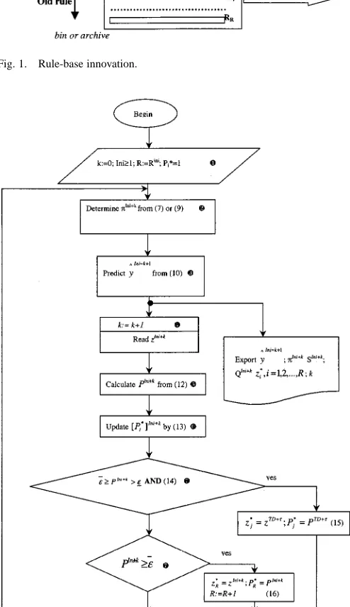
[image:5.612.314.538.64.167.2]Initially, the algorithm, as with the other approaches, uses a fixed set of rules as given in Section II. This is illustrated in Fig. 3 using the simplest two-dimensional case. The data avail-able initially are depicted with stars. They are described by five rules – , and the zone of influence of each rule is depicted by solid line circles in Fig. 3. Subsequently, new data samples are collected. They are depicted in Fig. 3 by “x” and “o” sym-bols. Each time a new data sample becomes available, its infor-mative potential (a reciprocal form of the Euclidean distance to all already available data) is calculated recursively by (12). The rules centers potentials are also updated recursively using (13).
Fig. 1. Rule-base innovation.
Fig. 2. Flow chart of the proposed identification algorithm.
On this basis, the mechanism for rule-base innovation and pa-rameters noniterative update is triggered when a data sample is found to represent some new feature, to the extent that estab-lishes a new rule in the model.
[image:5.612.303.550.141.569.2]Fig. 3. Rule-base evolution for a two-dimensional case.
In this way, the rule-base structure is gradually changed (one rule is replaced or a new one is added), while ensuring the inheritance of the vast majority of the rules (all except one are preserved till the next change). Effectively, this change of the rule-base structure is equivalent to a gradual innovation of the data space partitioning. Constant updates and checks of the potential of the new data samples, (12)–(17), are recursive, noniterative and, hence, very inexpensive computationally.
The new rule base is better suited to the changed data pat-tern, because it has both an up-dated structure (data-space parti-tioning) and parameters, while it inherits significant part of the old structure. It can be seen from Fig. 3 that in this illustrative example, the new model (bold dash–dotted line) represents the changed data pattern better then the old model (solid line), while preserving the character of the model. The replacement of rule by could be, for example, due to a saturation of , which could be difficult to be registered by the data available initially (data samples denoted by ‘x’).
IV. EXPERIMENTALRESULTS
The new algorithm has been tested on the Mackey–Glass chaotic time series prediction and the results compared to those generated by existing techniques, published in [5], [16], and [20]. A further component modeling example is demonstrated using data from air-conditioning equipment installed to serve a real building.
A. Mackey–Glass Chaotic Time Series Prediction
The chaotic time series is generated from the Mackey–Glass differential delay equation defined by [16], [20]
The problem is to use past values of to predict some future value of . The same example as published in [5], [16], and [20] has been adopted here to allow a comparison with the published results. Accordingly, , and the value of the signal six steps ahead is predicted based on the values of the signal at the current moment, six, 12 and 18 steps back
Output
Inputs
The data range of has also been adopted, with the first 500 samples forming the training data set and the second 500 forming the validation data set. The nondimensional error index (NDEI), used in [5], [16], and [20] has been calcu-lated to compare model performance.
The values of the thresholds used are given in (17). Since the number of data samples is low, there is no practical need of intro-ducing a moving window. The radii parameter ( ) re-mains a user-defined value that controls the generalization prop-erty and, respectively, the number of rules present in the model. The number of rules generated is also affected by the order of the new data and the data history. This is due to the relative nature of the thresholds, which depends on the specific data available at certain moment. Therefore, the results generated over the same training data set, but separated on initial and evolved parts are different.
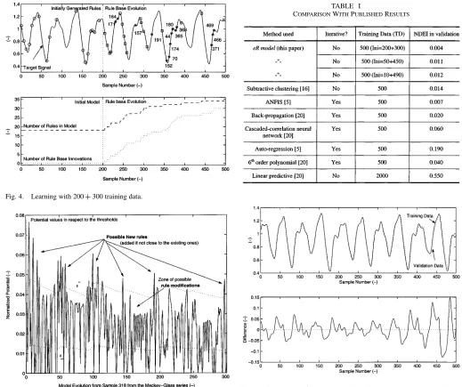
To generate comparable results to those already published, the first 500 data points were used to generate a model using the new approach. Part of the data was used to establish the initial model and the eR algorithm was left to run over the remaining data. Fig. 4 shows the model training for one of the trials, using 200 initial samples and 300 in evolving mode. The top plot shows the target series and details the sample-wise appearance of the rules and rule changes. The points highlighted with a circle show the initial model rule centers. The points marked with a square show new rules. The points marked by an asterisk show the rule base changes and the numbers represent the sample number of the rule that has been superceded by the new rule. The bottom plot gives an indication of the intensity of the rule base innovation over the training period. This rule-base innovation process has been driven by recursively calculated and updated potentials of the new data (samples from 318 to 617 from the Mackey–Glass series) illustrated in Fig. 5.
At the end of the training process, the resultant model was ap-plied to the validation data set, which was the second set of 500 unseen data (corresponding to the time series sample numbers from 618 to 1117). The NDEI was calculated for the model pre-dictions of the validation data and the results given in Table I. The results show that the new approach can yield a better model than the techniques which consider a fixed structure, improving the validation data model prediction NDEI significantly. The same procedure has been applied to trials with only 50 and 10 data initial samples and the rest (450 and 490, respectively) evolving mode. The initially generated model using subtractive clustering [16] based on 500 data samples was also used to pre-dict the validation data set. The higher NDEI compared to that after the incremental learning is evidence of the improvement of the model in terms of the identification and description of the process.
pro-Fig. 4. Learning with 200+ 300 training data.
Fig. 5. Potential values in respect to the thresholds.
posed approach to evolve the model starting form a very limited number of training data samples; a property extremely impor-tant in robotics and the design of autonomous systems.
One comment on the Mackey–Glass time-series as a bench-mark problem is that it has a distinctive periodic characteristic, demonstrated by the top plot of Fig. 6. This shows the target series used in training (samples 118 to 617) overlaid with the target series used in validation (samples 618 to 1117). The bottom plot of the same figure shows the difference between them. It is unlikely that a model having low error on training data will perform poorly on validation data that are almost the same. The problem is a well-known benchmark used in [5], [16], and [20], therefore, the new approach has been tested on it in order to compare performance with published approaches. The advantages of the eR modeling, however, become more obvious when the character of the data changes. This has been shown when the initial model has been built using only a small number of training data. This characteristic is further demonstrated by the following example.
TABLE I
COMPARISONWITHPUBLISHEDRESULTS
Fig. 6. Comparison of the Mackey–Glass time series training and validation data (samples 118 to 1117).
B. Air-Conditioning Heat Exchanger Modeling
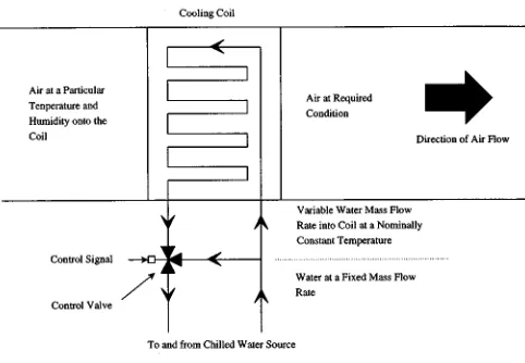
Air-conditioning systems generate comfortable indoor envi-ronments through the control of temperature and humidity. An important system component in the control of these properties is the cooling coil, a water-to-air heat exchanger. Fig. 7 shows a typical configuration. Air at various temperatures and humidi-ties is drawn over the coil. A desired air condition at the outlet is specified and the mass flow rate of chilled water, at a nomi-nally fixed temperature, is varied to achieve this condition. The operating point of the coil is largely dependent on the ambient (weather) conditions.
[image:7.612.32.551.62.497.2] [image:7.612.298.550.71.495.2]Fig. 7. Typical configuration of air-conditioning cooling coils.
the lack of experimental control that exists in typical measured data and the unexpected relationships between system compo-nents [26]. FRB models are a promising candidate for modeling these types of complex relationships.
Air-conditioning systems operating conditions are primarily dependent on seasonal variation in the ambient conditions. This means that it is often impractical to gather a set of fully representative data to train a globally applicable fuzzy model. Using data from one season only results in a model that is severely limited in its applicability. Such an approach would require repeated regeneration of the whole model when the data pattern changes. The evolving rule-based modeling approach is demonstrated here to be able preserving the core rules to autonomously restructure the model rule base so that the model can describe the new regions in the input data space and hence, generate precise predictions.
1) The Problem: The task is to model the characteristic tem-perature difference across a cooling coil based on the following measurements, depicted in Fig. 8:
• flow rate of the air entering the coil; • moisture content of the air entering the coil; • temperature of the chilled water;
• control signal to the valve.
The control signal positions the valve and controls the mass flow rate of chilled water through the coil. The signal can be used to infer the water mass flow rate in the model. In fact, using control signal as an input variable results in a model that charac-terizes the coil and control valve. All measurements and signals are time continuous and contain transients. The transients are not considered significant in the context of this paper, so they have been neglected to simplify the example.
[image:8.612.302.555.62.165.2]The data is from a full-scale air-conditioning test facility. Data from three months (May, July, and August) over two sea-sons (summer and spring) is shown in Fig. 9. The top plot shows the output data and the lower plots, the input data. The initial section of data was used to train the initial model. The data was generated for a July day by exciting the valve control signal over the whole range of operation. The data from the summer and spring days were collected with the system operating under normal conditions on days in August and May, respectively.
Fig. 8. The cooling coils model input and output relationship.
Fig. 9. The experimental data from a system serving a real building.
The initial model was generated using data from different sea-sons. This was then used to predict the summer and spring op-eration. The eR model generates predictions at each new data sample learning the information in the new data. The rule base was up-dated and the parameters re-estimated, as and when new information was detected in the data.
2) Results: Fig. 10 compares the performance of the initial model with the eR model, based on the data shown in Fig. 9. It should be noted that the scale of the -axis of the top plot is 40 times that of the bottom plot. The initial model was gen-erated using subtractive clustering on the initial 437 samples. The eR model uses the same parameter as in the above example (radii, values of thresholds. As the different operating seasons are presented to the initial model, the predictions are very poor, highlighting the weakness techniques with fixed structure have in terms of extrapolation. One way this could be resolved is by regenerating the whole model after data has been collected from the new operating regions.
[image:8.612.306.551.210.398.2]Fig. 10. Rule base evolution over the seasonal data.
Fig. 11. Prediction errors. The top and bottom plots show the initial model and the evolving model performance, respectively.
top plot refers the sample number whose coordinates formed the rule that has been superseded by the coordinates of the current data point. The bottom plot shows the sample-wise information about the rule base innovation.
The example demonstrates that it is likely that there will be some additional error present when abrupt changes occur in the operation characteristics. Such a condition will continue until sufficient data to from a new rule are observed. Slowly changing model environments are much less likely to cause the same ef-fects. The approach, however, is demonstrated to be able to cope with such dramatic changes.
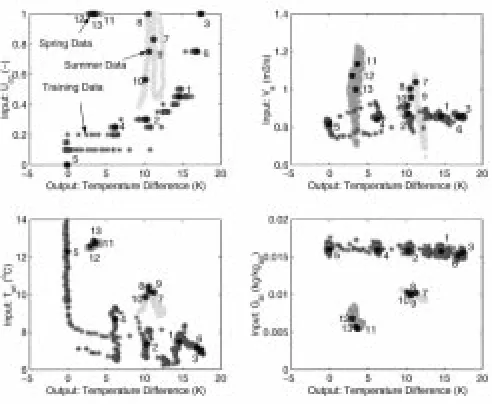
[image:9.612.46.281.302.489.2]The ability of the eR model to move into the new data regions is exemplified in Figs. 12 and 13. Fig. 12 depicts the regions of the input data space by plotting each one as function of the system output value. The three seasons are highlighted in dif-ferent shades of gray and the centers of the rules are in black, labeled with the rule number. The plot shows the rule descrip-tion of the training data. It also illustrates why the initial model is incapable of predicting the system performance in new data
Fig. 12. Regions of data input space and rule center location of the initial model.
Fig. 13. Regions of data input space and rule center location of the eR model.
regions. Fig. 13 shows the same plot after the structure evolu-tion. The rules have been changed clearly in favor of the new regions, resulting in significantly better prediction.
The results illustrates that in modeling of real objects val-idation on a limited range of data is not sufficient to guar-antee global applicability because behavior of the object or its environment could change significantly. Unseen regions of operating space that force extrapolation, result in unreliable model predictions. The new eR method has been demonstrated to overcome this significant problem.
V. CONCLUSION
[image:9.612.304.550.304.506.2]The adaptive nature of this eR model in addition to the highly transparent and compact form of fuzzy rules makes them a promising candidate for modeling and control of complex pro-cesses competitive to neural networks. This concept has been applied to the well-known benchmark problem (Mackey-Glass time series prediction) and it’s performance compared to other published algorithms. The ability of the approach to innovate the rule base to account for new regions of the system operating space as they are encountered has been demonstrated using an air-conditioning problem based on real data.
The approach has been demonstrated to give improved model based on the same number of data due to the different way of forming the model. The main advantages of the approach are as follows.
• It can develop/evolve an existing model when the data pat-tern changes, while inheriting the rule base.
• It can start to learn a process from a very low number of initial data samples and improve the performance of the initial model.
• It is noniterative and hence computationally very effective (the time necessary for calculation is a fraction of a second in Matlab environment running on a 550-MHz PC for each new data sample).
The proposed concept has wide implications for many fields, including nonlinear adaptive control, fault detection and diag-nostics, performance analysis of dynamical systems, time-series and forecasting, knowledge extraction, intelligent agents, intel-ligent buildings, behavior, and customized comfort modeling. The results illustrate the viability, efficiency and the potential of the approach when used with limited amount of initial information, especially important in autonomous systems and robotics.
ACKNOWLEDGMENT
The courtesy of ASHRAE for the use of data, generated from the ASHRAE funded research project RP1020, as well as the helpful comments of the referees and the Associate Editor, are acknowledged.
REFERENCES
[1] R. R. Yager and D. P. Filev, “Learning of fuzzy rules by mountain clus-tering,” in Proc. SPIE Conf. Application of Fuzzy Logic Technology, Boston, MA, 1993, pp. 246–254.
[2] L. Ljung, System Identification, Theory for the User. Upper Saddle River, NJ: Prentice-Hall, 1987.
[3] R. R. Yager and D. P. Filev, Essentials of Fuzzy Modeling and Control, NY: Wiley, 1994.
[4] T. A. Johanson and R. Murray-Smith, “Operating regime approach to nonlinear modeling and control,” in Multiple Model Approaches to
Mod-eling and Control, R. Murray-Smith and T. A. Johanson, Eds. Hants, U.K.: Taylor Francis, 1998, pp. 3–72.
[5] J. S. R. Jang, “ANFIS: Adaptive network-based fuzzy inference sys-tems,” IEEE Trans. Syst., Man, Cybern., vol. 23, pp. 665–685, June 1993.
[6] C. K. Chiang, H.-Y. Chung, and J. J. Lin, “A self-learning fuzzy logic controller using genetic algorithms with reinforcements,” IEEE Trans.
Fuzzy Syst., vol. 5, pp. 460–467, 1996.
[7] P. P. Angelov, V. I. Hanby, R. A. Buswell, and J. A. Wright, “Automatic generation of fuzzy rule-based models from data by genetic algorithms,” in Advances in Soft Computing, R. John and R. Birkenhead, Eds. New York: Springer-Verlag, 2001, pp. 31–40.
[8] F. Hoffmann and G. Pfister, “Learning of a fuzzy control rule base using Messy genetic algorithms,” in Studies in Fuzziness and Soft Computing, Herrera and Verdegay, Eds. Heidelberg, Germany: Physica Verlag, 1996, vol. 8, pp. 279–305.
[9] P. Angelov, Evolving Rule-Based Models: A Tool for Design of
Flex-ible Adaptive Systems, In the Series Studies in Fuzziness and Soft Com-puting. Heidelberg, Germany: Springer, Physica-Verlag, 2002, vol. 92, pp. 1–213.
[10] B. Carse, T. C. Fogarty, and A. Munro, “Evolving fuzzy rule-based con-trollers using GA,” Fuzzy Sets Syst., vol. 80, pp. 273–294, 1996. [11] P. Angelov and R. Guthke, “A GA-based approach to optimization of
bioprocesses described by fuzzy rules,” J. Bioprocess Eng., vol. 16, pp. 299–301, 1997.
[12] K. Shimojima, T. Fukuda, and Y. Hasegawa, “Self-tuning fuzzy mod-eling with adaptive membership function, rules and hierarchical struc-ture based on genetic algorithm,” Fuzzy Sets Syst., vol. 71, pp. 295–309, 1995.
[13] T. Takagi and M. Sugeno, “Fuzzy identification of systems and its appli-cation to modeling and control,” IEEE Trans. Syst., Man, Cybern., vol. SMC-15, pp. 116–132, 1985.
[14] W. Pedrycz, “An identification algorithm in fuzzy relational systems,”
Fuzzy Sets Syst., vol. 13, pp. 153–167, 1984.
[15] P. P. Angelov, V. I. Hanby, and J. A. Wright, “HVAC systems simulation: A self-structuring fuzzy rule-based approach,” Int. J. Arch. Sci., vol. 1, no. 1, pp. 49–58, 2000.
[16] S. L. Chiu, “Fuzzy model identification based on cluster estimation,” J.
Intell. Fuzzy Syst., vol. 2, pp. 267–278, 1994.
[17] J. Bezdek, “Cluster validity with fuzzy sets,” J. Cybern., vol. 3, no. 3, pp. 58–71, 1974.
[18] F.-J. Lin, C.-H. Lin, and P.-H. Shen, “Self-constructing fuzzy neural net-work speed controller for permanent-magnet synchronous motor drive,”
IEEE Trans. Fuzzy Syst., vol. 9, pp. 751–759, Oct. 2001.
[19] “EUNITE: European Network on Intelligent Technologies for Smart Adaptive Systems,”, Contract IST-2000-29 207, 2000.
[20] R. S. Crowder, “Predicting the Mackey-Glass timeseries with Cas-cade-correlation learning,” in Proc. of Connectionist Models Summer
School, D. Touretzky, G. Hinton, and T. Sejnowski, Eds. Pittsburgh, PA: Carnegie Mellon University, 1990, pp. 117–123.
[21] H. R. Berenji, “A reinforcement learning-based architecture for fuzzy logic control,” Int. J. Approx. Reason., vol. 6, pp. 267–292, 1992. [22] G. G. Yen and P. Meesad, “An effective neuro-fuzzy paradigm for
ma-chinery condition health monitoring,” in Proc. IEEE Int. Joint Conf.
Neural Networks, Washington, DC, 1999, pp. 1567–1572.
[23] D. E. Gustafson and W. C. Kessel, “Fuzzy clustering with a fuzzy co-variance matrix,” in Proc. IEEE Control Decision Conf., San Diego, CA, 1979, pp. 761–766.
[24] F. Klawon and P. E. Klement, “Mathematical analysis of fuzzy classi-fiers,” Lecture Notes Comput. Sci., vol. 1280, pp. 359–370, 1997. [25] A. Dexter and J. Pakenen, “Demonstrating automated fault detection and
diagnosis in real buildings,” VTT Building Technology, Espoo, Finland, 2001.
[26] R. A. Buswell, “Uncertainty in the first principle model based condition monitoring of HVAC systems,” Ph.D. dissertation, Loughborough Univ., Leicestershire, U.K., 2001.
[27] K. L. Anderson, G. L. Blackenship, and L. G. Lebow, “A rule-based adaptive PID controller,” in Proc 27th IEEE Conf. Decision Control, 1988, pp. 564–569.
[28] P. Strobach, Linear Prediction Theory: A Mathematical Basis for
Adap-tive Systems. New York: Springer-Verlag, 1990.
[29] D. P. Filev, T. Larsson, and L. Ma, “Intelligent control for automotive manufacturing-rule based guided adaptation,” in IEEE Conf.
IECON-2000, Nagoya, Japan, Oct. IECON-2000, pp. 283–288.
[30] R. Babuska, H. B. Verbruggen, and H. Hellendoorn, “Promising fuzzy modeling and control methodologies for industrial applications,” in
Plamen Angelov (M’99) received the Ph.D. degree from the Bulgarian Academy of Science in 1993.
Currently, he is a Research Fellow at Loughbor-ough University, Leicestershire, U.K. He has been a Visiting Research Fellow at CESAME, Catholic University of Louvain, Louvain, Belgium (1997), and Hannover and Jena, Germany (1995–1996). His research interests are in computational intelligence related to the control theory, particularly in evolving rule-based models, self-organizing and autonomous systems, evolutionary algorithms, optimization and optimal control in a fuzzy environment, neural networks and hybrid models, knowledge extraction, and accumulation. Engineering applications to indoor climate control systems, biotech processes, risk assessment, electrical load forecasting, etc. have also been studied and attracted his research interest. He is the author of the monograph Evolving Rule based Models: A Tool for Design
of Flexible Adaptive Systems (Heidelberg, Germany: Springer, Physica-Verlag,
2002).
Dr. Angelov has been on the Program and Organizing Committees of a number of Conferences (GECCO-2002, RASC-2002, FUBEST’94 and ’96, BioPS’94, ’95, ’97), and has a research portfolio with a wide range of funding sources: the European Commission, the American Society for Heating Refrigerating and Air-Conditioning Engineers, Research Councils of U.K. (EPSRC), Germany (DAAD and DFG), Belgium, Italy (CNR), and Bulgaria (NFSI), and a number of industrial sponsors.
Richard Buswell received the B.Eng. (Hons.) degree in environmental systems engineering and the Ph.D. degree from Loughborough University, Leicestershire, U.K., in 1996 and 2001, respectively. His Ph.D. work considered the uncertainty present in modeling real systems.