Frequency Time Analysis (FTAN) and Moment Tensor Inversion Solutions from Short Period Surface Waves in Cameroon (Central Africa)

Published Online February 2014 (http://www.scirp.org/journal/ojg) http://dx.doi.org/10.4236/ojg.2014.42004

Frequency Time Analysis (FTAN) and Moment Tensor

Inversion Solutions from Short Period Surface Waves in

Cameroon (Central Africa)

Eric N. Ndikum1,2*, Charles T. Tabod1, Alain-Pierre K. Tokam1 1

Department of Physics, University of Yaounde 1, Yaounde, Cameroon 2

Department of Fundermental Sciences, H.T.T.T.C. Bambili-Bamenda, The University of Bamenda, Bambili, Cameroon Email: [email protected]

Received December 26, 2013; revised January 20, 2014; accepted January 28, 2014

Copyright © 2014 Eric N. Ndikum et al. This is an open access article distributed under the Creative Commons Attribution License, which permits unrestricted use, distribution, and reproduction in any medium, provided the original work is properly cited. In accor-dance of the Creative Commons Attribution License all Copyrights © 2014 are reserved for SCIRP and the owner of the intellectual property Eric N. Ndikum et al. All Copyright © 2014 are guarded by law and by SCIRP as a guardian.

ABSTRACT

Short period surface waves generated by a local earthquake recorded by broadband seismometers at distances of about 186 to 778 km from the earthquake’s epicenter located in Cameroon (Central Africa) were processed for group velocity maps and dispersion waveforms using the frequency time analysis (FTAN) method. The resulting group velocity fundamental modes of the extracted Rayleigh and Love waves were used for a joint amplitude spectral and P polarity inversion using moment tensor inversion. The corresponding group velocity dispersion curves, the residual as a function of depth, the amplitude spectra and the moment tensor solutions of the regions from the epicenter to the different stations up to a depth of about 10 km were obtained.

KEYWORDS

Frequency Time Analysis (FTAN); Surface Waves; Group Velocity Dispersion Curves; Moment Tensor Inversion

1. Introduction

Information on the constitution of the subsurface struc- ture of the earth can be obtained from the studies of elas- tic waves travelling through the earth which are generat- ed by either natural phenomena like earthquakes and collapse of rock cavities or by artificial means like ex- plosions from nuclear test sites. Also, down- and cross- hole tests can be used to obtain detailed shear wave (Vs) velocities even though these are very expensive because of drilling costs [1]. Consequently, they can be measured from refraction seismic surveys by studying the disper- sion of Rayleigh surface wave group velocities which are related to the signal energy. One very efficient method to study surface waves is the frequency time analysis (FTAN) method which is very useful in defining Vs pro- files of shallow geological structures [2] and finds a lot of applications in Seismology. In this paper, FTAN is used to extract group velocity dispersion curves of sur-

face wave fundamental modes resulting from a local earthquake, after which inversion is carried out on the results using the moment tensor inversion technique.

2. Methodology

2.1. Data Acquisition

Figure 1. Positions of epicenter (star) of Monatele earth- quake and seismic stations (squares).

Table 1. Distances of seismic stations from earthquake epi-center.

Seismic station Distance from earthquake epicenter (km)

CM06 229.2

CM09 186.3

CM18 230.6

CM24 431.9

CM26 421.6

CM29 603.8

CM32 778.8

installed in January 2005 and used in the Cameroon Broadband Seismic Experiment in which studies on the Cameroon Volcanic Line (CVL) were carried out [3]. These 7 seismometers were constituted of two (2) Guralp CMG-3T seismometers, one (1) Guralp CMG-3ESP seismometer and four (4) Streckeisen STS-2 seismome- ters. They recorded data continuously at 40 samples per second [4].

2.2. The Frequency Time Analysis (FTAN) Method

The frequency time analysis (FTAN) method which was put in place by Levshin and associates [5,6] came to im-prove in a significant way the multiple filter analysis which Dziewonski and associates originally developed [7]. FTAN can be applied in a setting with only a single channel to measure group velocity even when there is higher mode contamination. When the source is known, the phase velocity can also be measured [2].

This method employs a system of narrow-band Gaus- sian filters, with varying central frequency, that do not

introduce phase distortion and give a good resolution in the time-frequency domain.

For each filter band the square amplitude of the in- verse FFT of the filtered signal is the energy carried by the central frequency component of the original signal. Since the arrival time is inversely proportional to group velocity, for a known distance, the energy is obtained as a function of group velocity at a certain central frequency. The process is repeated for different central frequencies. A FTAN map is the image of a matrix whose columns are the energy values at a certain period and the rows are the energy values at constant group velocity. A sequence of frequency filters and time window is applied to the dispersion curve for an easy extraction of the fundamen- tal mode. The floating filtering technique, combined to a phase equalization, permits to isolate the fundamental mode from the higher modes [1,8].

FTAN is useful in defining VS profiles of shallow geological structures and has been applied with great success in both seismological and engineering fields [9-11].

2.3. Moment Tensor & Source Depth Inversion Method

The theory behind Moment Tensor & Source Depth In- version is summarized below and the details are found in the reference manual of the Moment Tensor & Source Inversion Program which is located in the web site of Surface waves processing & seismic source inversion (double-couple approximation) [12].

The moment tensor M can be used to describe an in- stant point source. A double couple instant point source at a depth h, can be given by the following: double couple depth, its focal mechanism which is characterized by three angles: strike, dip and slip or by two unit vectors (direction of principal tension T and direction of princip- al compression P) and seismic moment M0. M0 is deter-

mined through the minimisation of the misfit between observed and calculated surface wave amplitude spectra for every current combination of all other parameters. A relationship between the spectrum of the displacements in any surface wave and the total moment tensor M is given as:

(

)

(

)

, , ,

i ij ij

i

x M G x y

i y

µ ω ω

ω

 ∂ 

= _{ }

∂

  (1)

waves are used for determining source parameters under consideration while observed surface wave phase spectra are used only for very long periods. Equation (1) can be used to calculate the amplitude spectra of surface waves. A comparison of calculated and observed amplitudes spectra gives a residual ε( )i for every point of observa- tion, every wave and frequency.

Surface wave amplitude spectra inversion:If all cha- racteristics of the medium are known the representation (1) gives us a system of equations for parameters defined above. Let us consider now a grid in the space of these 4 parameters. Let the models of the media be given. Using formula (1) we can calculate the amplitude spectra of surface waves at the points of observation for every possible combination of values of the varying parameters. Comparison of calculated and observed amplitude spec- tra give us a residual ε( )i for every point of observation, every wave and every frequency ω. For any observed value of the spectrum u( )i

( )

( )

₍

₎

i

u xω |, where i = 1,…,N; the nor- malised amplitude residual is defined by:

(

)

₍

₎

h T P u x

ε φ ε ω

= =

   

= _  _{ } _



∑

∑

The residual can then be defined such that one is a function of a scalar argument εh

( )

( )

( )

Since four different focal mechanisms will radiate the same surface wave amplitude spectra, the focal mechan- ism can not be uniquely determined from surface wave amplitude spectra. Consequently, long period spectra of surface waves or polarities of P wave first arrivals can be used to obtain a unique solution for the focal mechanism. Joint inversion of surface wave amplitude and phase spectra:For a given frequency range the phase spectra of surface waves at the points of observation for every possible combination of values of the varying parameters can be calculated using Equation (1). When the calcu- lated and observed phase spectra are compared, a resi- dual ε( )_phi for every point of observation, every wave and every frequency ω can be gotten. The normalised am- plitude residual is given by:

(

)

1 1 , , , N i amp ph i

h T P N

ε φ ε

=

  

= _{  }

∏ 

∑

The joint residual is given as:

(

)(

)

1 1 _ph 1 _amp

ε= − −ε −ε (4)

Joint inversion of surface wave amplitude spectra and P wave polarities:When the calculated radiation pattern of P waves for every current combination of parameters are compared with observed polarities, the misfit ob- tained is used to calculate a joint residual of surface wave

amplitude spectra and polarities of P wave first arrivals. if εamp is the residual of surface wave amplitude spec-

tra and εP—the residual of P wave first arrival polari-

ties (the number of wrong polarities divided by the full number of observed polarities), then:

(

)(

)

1 1 _p 1 _amp

ε= − −ε −ε (5)

3. Data Analysis

The data base creator (dbcreator) program, frequency time analysis (FTAN) program and the moment tensor and source depth inversion program used to analyse data in this paper were obtained from the website of Surface waves processing & seismic source inversion [15].

A seismic database in AH binary file format was created from seismic data in SEED format recorded by the broadband seismometers CM06, CM09, CM18, CM24, CM26, CM29 and CM32 located around Came- roon, Central Africa (see Figure 1) using the dbcreator program. The condition of sampling the database was set such that the input time series was decimated to a binary time series of 1 count per second. This database had a signal length of 120 minutes, being the maximum length provided for by the program.

The FTAN program was then used to process the seismic signal in the database for each station choosing the most appropriate bandpass filtering parameters (see

Table 2) that permitted the best extraction of the funda- mental mode. To the fundamental mode of each signal, parameters for the right bounds (group velocity and pe- riod) for the FTAN diagram were then chosen (see Table 3) in order to extract the group velocity dispersion curve.

This was done using the floating filtering technique combined to phase equalization. For each station, ac- ceptable results of the filtered signal, the amplitude spec- tra, the FTAN calculated group velocity diagram and the FTAN maps of the filtered seismograms were generated and saved. The different period ranges from floating fil- tering were saved (see Table 4) to be used for inversion.

Table 2. Bandpass filtering parameters applied on surface waves in FTAN.

Seismic stations

Bandpass filtering parameters (s)

Short periond zero Short period corner Long period corner Long period zero

CM06 7 11 20 25

CM09 5 9 20 25

CM18 7 10 25 30

CM24 7 11 25 30

CM26 7 11 25 30

CM29 10 13 25 30

CM32 14 23 40 50

Table 3. Parameters for the bounds of the FTAN diagram.

Seismic stations Parameters for FTAN diagram

CM06 Group velocity (km/s) 1.5 5.0

Period (s) 5 25

CM09 Group velocity (km/s) 1.5 5.0

Period (s) 2 25

CM18 Group velocity (km/s) 1.5 5.0

Period (s) 3 30

CM24 Group velocity (km/s) 1.5 5.0

Period (s) 7 30

CM26 Group velocity (km/s) 1.5 5.0

Period (s) 7 30

CM29 Group velocity (km/s) 1.5 5.0

Period (s) 9 30

CM32 Group velocity (km/s) 1.5 5.0

Period (s) 10 50

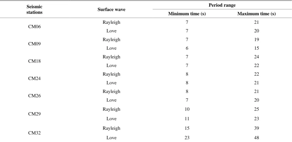
Table 4. Resulting period ranges from floating filtering.

Seismic

stations Surface wave

Period range

Minimum time (s) Maximum time (s)

CM06 Rayleigh 7 21

Love 7 20

CM09 Rayleigh 7 19

Love 6 15

CM18 Rayleigh 7 24

Love 7 22

CM24 Rayleigh 8 22

Love 8 21

CM26 Rayleigh 8 21

Love 7 20

CM29

Rayleigh 10 25

Love 11 23

CM32

Rayleigh 15 39

leigh and Love dispersion waves (with the minimum and maximum time in the spectral range being 7 and 48 s) and then only for the Rayleigh dispersion waves alone (with the minimum and maximum time in the spectral range being 7 and 39 s).

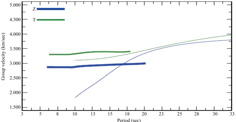
4. Results

When Ftan program was applied to each of the stations using the different parameters for bandpass filtering,

bounds for the FTAN diagram, and period range shown in Tables 2, 3 and 4, the best solutions for each station was retained. These solutions were saved for the ampli- tude spectra, the group velocity diagram, the FTAN map and the filtered (cleaned) seismograms. FTAN results were obtained for all the seven stations and the results for station CM18 are presented here in Figures 2, 3, 4 and

5.

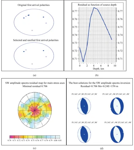
When the moment tensor and source depth inversion

Figure 2. Amplitude spectra for CM18 (thin lines represent the amplitude spectra of raw signals; thick lines represent the amplitude spectra of cleaned signals).

Figure 4. Plot of filtered signals for CM18 (red for Rayleigh and green for love) and raw signal (blue).

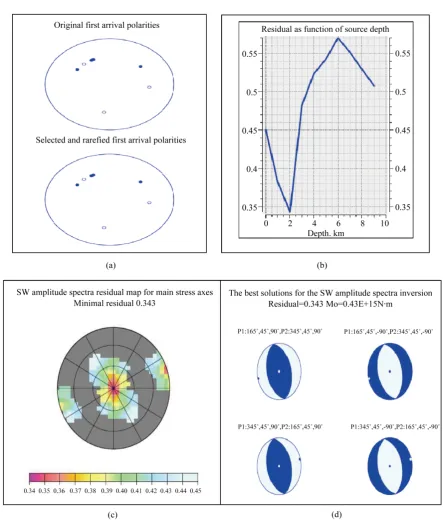
program was applied on the dispersion signals from both the Rayleigh and Love waves, the selection and rarefica- tion of polarity data were carried out at angles of polarity data smoothing of 1, 5 and 10 degrees, but all the results from these were the same. In the case where the moment tensor and source depth inversion program was applied to both Rayleigh and Love waves, results of amplitude spectra inversion and those of joint amplitude spectra plus P polarity inversion were obtained (for the polarities

before and after selection and rarefication, the residual as a function of source depth, the spectral residual map for main stress axis, and moment tensor solutions) and pre- sented in Figures 6(a), (b), (c), (d) and Figures 7(a), (b),

(c), (d) respectively.

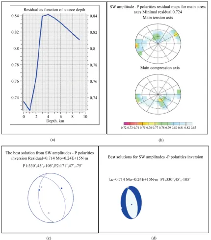
In like manner, for the case where the moment tensor and source depth inversion program was applied to only Rayleigh waves, results of amplitude spectra inversion and those of joint amplitude spectra plus P polarity

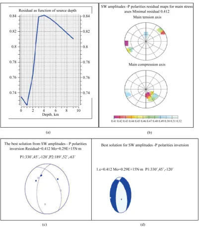
Figure 7. Results of amplitude spectra plus P polarity inversion on both Rayleigh and love waves: (a) Plot of residual as func-tion of source depth; (b) Plot of residual for main stress axis; (c) and (d) Representafunc-tion of the best moment tensor solufunc-tions.

inversion were also obtained and presented in Figures 8(a),

(b), (c), (d) and Figures 9(a), (b), (c), (d) respectively.

5. Discussion of Results

The results from moment tensor inversion presented in

Figures 6(a), (b), (c), (d) to 9(a), (b), (c), (d) above in- dicate that for an inversion carried out on both Rayleigh and Love waves, surface wave amplitude spectral inver- sion has residual and scalar seismic moment (Mo) values

Figure 8. Results of amplitude spectra inversion on Rayleigh waves only: (a) Plot of polarities before and after selection and rarefication, (b) Plot of residual as function of source depth, (c) Plot of residual for main stress axis, (d) Representation of the best moment tensor solutions.

it can be noticed that results of the amplitude spectra inversion were improved upon by the joint amplitude spectra and P polarity inversion as far as the precision in moment tensor solutions generated is concerned.

6. Conclusion

After using the FTAN program to extract the surface

Figure 9. Results of amplitude spectra plus P polarity inversion on Rayleigh waves only; (a) plot of residual as function of source depth, (b) plot of residual for main stress axis, (c) and (d) representation of the best moment tensor solutions.

and scalar seismic moment (Mo) values of 0.714 and

0.24E+15 Nm respectively.

REFERENCES

[1] M. Natale, C. Nunziata and G. F. Panza, “FTAN Method for the Detailed Definition of vs in Urban Areas,” 13th World Conference on Earthquake Engineering, Vancou-ver, 1-6 August 2004, Paper No. 2694.

[2] J. Boaga, “Seismic Noise and Controlled Source Surveys: Tools for Seismic Hazard Deterministic Approach,” Ph.D. dissertation, University of Padova, Padova, 2008.

[3] G. G. Euler, D. A. Wiens, P. Shore, F. W. Koch, R. Tibi,

A. A. Nyblade and A. M. Reusch, “Shear Velocity Structure of the Cameroon Volcanic line Region from Rayleigh Wave Phase Velocities,” EOS, Transactions, American Geophysical Union, 89(53), AGU Fall Meeting Suppl., 2008, Abstract #S21C-1843.

[4] K. A. P. Tokam, C. T. Tabod, A. A. Nyblade, A. Julia, D. A. Weins and M. E. Pasyanos, “Structure of the Crust Beneath Cameroon, West Africa, from the Joint Inversion of Rayleigh Wave Group Velocities and Receiver Func-tions,” Geophyiscal Journal International, Vol. 183, No. 2, 2010, pp. 1061-1076.

http://dx.doi.org/10.1111/j.1365-246X.2010.04776.x

Geophysicae, Vol. 128, No. 2, 1972, pp. 211-218.

[6] A. Levshin, L. I. Ratnikova and J. Berger, “Peculiarities of Surface Wave Propagation across Central Eurasia,” Bulletin of the Seismological Society of America, Vol. 82, No. 6, 1992, pp. 2464-2493.

[7] A. Dziewonski, S. Bloch and M. Landisman “A Tech-nique for the Analysis of Transient Seismic Signals,” Bulletin of the Seismological Society of America, Vol. 59, No. 1, 1969, pp. 427- 444.

[8] L. I. Ratnikova, “Frequency-Time Analysis of Surface Waves,” In: Workshop on Earthquake Sources and Re-gional Lithospheric Structures from Seismic Wave Data, International Centre for Theoretical Physics, Trieste, 1990, pp. 1-12.

[9] C. Nunziata, G. Costa, M. Natale and G. F. Panza, “FTAN and SASW Methods to Evaluate vs of Neapolitan Pyroclastic Soils,” Earthquake Geotechnical Engineering (Balkema), Vol. 1-3, 1999, pp. 15-19.

[10] C. Nunziata, G. Costa, M. Natale, A. Vuan and G. F. Panza, “Shear Wave Velocities and Attenuation from Rayleigh Waves,” In: Pre-Failure Deformation Characte-ristics of Geomaterials (Balkema), 1999, pp. 365-370.

[11] C. Nunziata, G. Costa, M. Natale and G. F. Panza, “Seis-mic Characterization of the Shore Sand at Catania,” Journal of Seismology, Vol. 3, No. 3, 1999, pp. 253-264.

http://dx.doi.org/10.1023/A:1009861824955

[12] A. Z. Mostinskiy and B. G. Bukchin, “Moment Tensor & Source Depth Inversion Program Reference Manual, Sur-face Waves Processing & Seismic Source Inversion,” In-ternational Institute of Earthquake Prediction Theory and Mathematical Geophysics (Mitpan), On-Line Bulletin, 1998-2005.

http://www.mitp.ru/en/soft/word_pdf_Manuals/MomTens _man.pdf‎

[13] A. L. Levshin, “Effects of Lateral Inhomogeneity on Sur-face Wave Amplitude Measurements,” Annles Geophysi-cae, Vol. 3, No. 4, 1985, pp. 511-518.

[14] B. G. Bukchin, “Determination of Source Parameters from Surface Waves Recordings Allowing for Uncertain-ties in the ProperUncertain-ties of the Medium,” Izvestiya Physics of the Solid Earth, Vol. 25, 1990, pp. 723-728.

[15] A. Z. Mostinskiy, B. G. Bukchin and A. A. Egorkin, “Software Packages for Data Base, Frequency-Time Analysis Program and Moment Tensor & Source Depth Inversion Program (FMT package), Surface Waves Processing & Seismic Source Inversion (Double-Couple Approximation),” International Institute of Earthquake Prediction Theory and Mathematical Geophysics (Mit-pan), On-Line Bulletin, 1998-2005.