Calculation of IMAGE/MENA geometric factors and conversion of images to units of integral and differential flux

Calculation of IMAGE/MENA geometric factors and conversion of images

to units of integral and differential flux

M. G. Henderson,a兲 M. F. Thomsen, R. Skoug, M. H. Denton, R. Harper, and H. O. Funsten

ISR-1, Los Alamos National Laboratory, Los Alamos, New Mexico 87545

C. J. Pollock

Southwest Research Institute, San Antonio, Texas

共Received 13 October 2004; accepted 1 February 2005; published online 1 April 2005兲

The Medium Energy Neutral Atom共MENA兲instrument flown on the NASA IMAGE spacecraft is a time-of-flight neutral particle imager designed to image energetic neutral atom emissions from the Earth’s inner magnetosphere over an energy per mass range of 1 – 60 keV/ amu. Images are generated by combining data from three separate heads and have a nominal angular resolution of 4 °⫻4°. Here, we present a first-principles calculation of the geometric factors for each of the start-byte/stop-byte combinations for each of the three heads in the IMAGE/MENA instrument based on a detailed understanding of the its physical construction. The geometric factors are used to compute combined integral flux images and it is demonstrated that they result in head-to-head matching of the data that are both continuous and physically reasonable. We also discuss several issues associated with energy binning as a means for constructing differential flux images and present a powerful and robust approach that solves several critical problems inherent with this type of instrument. © 2005 American Institute of Physics. 关DOI: 10.1063/1.1884190兴

I. INTRODUCTION

The Medium Energy Neutral Atom共MENA兲instrument on the IMAGE spacecraft1was designed to image the ener-getic neutral atom 共ENA兲 emissions from the earth’s mag-netosphere over an energy-per mass range of 1 – 60 keV/ amu with a nominal angular resolution of 4 °⫻4°. The instrument is comprised of a set of three 共nominally兲 identical sensor “heads” with head 2 pointing perpendicular to the spacecraft spin axis and heads 3 and 1 offset by ±20° with respect to the perpendicular direction. Photographs of the MENA instru-ment mounted on the IMAGE spacecraft and also in the laboratory during calibration are shown in Figs. 1共a兲 and 1共b兲. In panel共a兲, the spin axis of the spacecraft points to-ward the top of the page, and the MENA instrument is marked with an arrow. From left to right the heads are iden-tified as: head 3, head 2, and head 1. The heads image only in the polar angle direction共with respect to the spin axis兲and are collimated in the azimuthal direction 关the transmission probability in the azimuthal direction has a full width at half maximum共FWHM兲of approximately ±4°兴. Imaging in the azimuthal direction is facilitated by the rotation of the space-craft 共the spin period is nominally 120 s兲. Three heads are required in order to increase the total field of view共FOV兲in the polar angle direction and in order to fill in the central gaps in coverage in each head.

A schematic illustration of the imaging concept for a single head is shown in Fig. 1共d兲. Incident ENAs are initially collimated in azimuth by a set of 21 curved parallel plates.

These plates are alternately biased with high voltage共on the order of 3 kV兲in order to sweep out ions with energies up to about 20 keV. An ENA must then pass through a freestand-ing transmission gratfreestand-ing nano-structure designed to transmit heavy particles but reject UV photons. Following this, the ENA passes through a thin carbon foil共mounted on the bot-tom side of the grating structure兲. ENAs exiting the foil gen-erate secondary electrons that we call “start electrons.” These electrons are accelerated by a grid which causes them to move very rapidly downward to the microchannel plate 共MCP兲 detector in a z-stack configuration that subsequently generates a “start pulse” on a “start” position-sensitive an-ode. Meanwhile, the ENA continues on in a straight line path to impact the MCP detector and generates a “stop” pulse on the stop position-sensitive anode. Although they are mounted on a single board, the start and stop anodes are physically separated and electrically isolated, each having its own pro-cessing electronics. The stop anode lies on both sides of the start anode, and the two halves of this split anode are elec-trically coupled. The total variation in gain across the MCP is

⬍10%.1

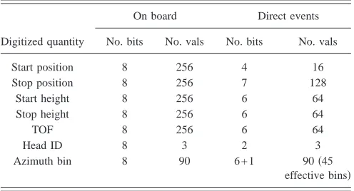
The quantities that are measured and reported for the detection of and ENA are: start position, stop position, start pulse height, stop pulse height, time of flight 共TOF兲, head identification 共ID兲, and the 4°-wide azimuthal sector in which the event occurred. The TOF is measured as the time difference between the start pulse and the stop pulse. On board the spacecraft, these quantities are all described using 8 bit words and the on-board image processing can take ad-vantage of the full digital resolution. However, the direct-events data that get telemetered to the ground have a reduced resolution. In the direct events data or “statistics data,” the

a兲_{Author to whom correspondence should be addressed; electronic mail:}

[email protected]

byte values are down sampled as shown in Table I. A further complication is that, due to telemetry constraints, only a sub-set of the measured direct events can be included in the tele-metered direct events data set共typically we receive no more than⬇13 000 events per spin on the ground兲.

For the azimuth bin, the direct events data contain a 6 bit coarse resolution word specifying an 8°-wide azimuth bin, plus a 1 bit word indicating whether the event occurred in the lower 4° portion of the 8° bin or the upper 4° portion of the 8° bin. However, since the size of the telemetry buffer allocated for MENA typically allows for the storage of no more than⬇13 000 direct events共per spin兲there is a limited number of events that can be reported back to the ground in one spin of the spacecraft. Thus the quota of reported events is usually spent on those that occurred in the lower half of the coarse bin. This unfortunately limits the azimuthal reso-lution of the direct events data to just 8° or 45 bins per spin as indicated by the bracketed quantity in Table I.

In addition to the direct events data, we also receive on the ground the total singles counts for start, stop, and valid 共coincidence兲events in each head accumulated over an entire spin. These quantities allow us to scale the direct event count rates up to what was observed on board—although this scal-ing process does not compensate for the poorer countscal-ing statistics inherent in the direct-events data.

Before launch it was anticipated that the measured

quan-tities would be used as follows. First, the start and stop po-sitions would be used to determine the incident angle,␰. The TOF and incident angle would be used to determine the speed. The pulse heights were then supposed to allow for resolution of mass 共e.g., H or O兲. And finally the energy would be determined from the mass and speed. In practice, this scheme works very well except that so far, we have not been successful in using the pulse heights to extract species information. Thus, for the time being we assume that all the ENAs are hydrogen. However, as we shall see later in this document, there is still a chance that we may yet be able to separate hydrogen and oxygen in the direct-events data.

A much more detailed description of the MENA instru-ment can be found elsewhere.1 In this document, we focus specifically on the process of converting the raw direct-events data into images with units of integral and differential flux. In doing so, we present a first-principles calculation of the MENA geometric factors based on a detailed understand-ing of the physical design of the instrument. Followunderstand-ing this, we discuss issues associated with energy binning and we present a solution that not only overcomes these issues, but also offers the possibility of extracting species information as well.

II. CONVERTING FLUX TO COUNTS

Following the formalism of Sullivan,2 the coincidence counting rate obtained with a particle telescope can be writ-ten

C =1 T

冕

0

t₀+T

冕

冕

冕

⫻

兺

s

␶s共E,␴,uˆ,t兲js共E,uˆ,t兲uˆ · d␴dt d␻dE 共1兲 where,

C ⫽ coincidence counting rate共s−1兲;

T ⫽ total observing time共s兲;

t0 ⫽ time at start observation, s ⫽ species label,

␶s ⫽ overall detection efficiency for particles of species s. It can very as a function of energy, look direction detection location and time;

js ⫽ incident differential flux for species s 共cm−2_sr−1_keV−1_s−1_兲;

uˆ ⫽ look direction; TABLE I. Hardware byte down sampling.

Digitized quantity

On board Direct events

No. bits No. vals No. bits No. vals

Start position 8 256 4 16

Stop position 8 256 7 128

Start height 8 256 6 64

Stop height 8 256 6 64

TOF 8 256 6 64

Head ID 8 3 2 3

Azimuth bin 8 90 6 + 1 90共45

effective bins兲

␴ ⫽ element of surface area in the final detector element;

uˆ · d␴ ⫽ element of projected area as seen from the look direction uˆ,

d␻ ⫽ element of solid angle共sin␪d␪d␾in spheri-cal polar coordinates兲;

S ⫽ domain of integration over ␴ 共i.e., the sur-face of the final detector element兲;

⍀ ⫽ domain of integration over solid angle 共 de-pends on geometry of the various elements兲; and

E ⫽ domain of integration over energy.

Sullivan2 used this expression analytically for straight line particle trajectories that make it through the apertures to the detector. However, it can also be evaluated共e.g., via Monte Carlo integration兲for more complex trajectories共e.g., curved trajectories of charged particles in a magnetic field兲. In addi-tion, Tuszewski, Cayton, and Ingraham3 have recently ex-tended Sullivan’s formalism to analytically include more complicated particle trajectories that can contribute to the count rate despite the fact that they do not necessarily pass through the geometrical apertures. This newer “analytical probability”共AP兲approach can account for features such as penetrating particles, scattering, reflections and secondary bremsstrahlung photons. Although in future work we may need to include some of these more complicated effects, here we will restrict our calculations to simple straight-line trajec-tories that have a clear geometrical path through the aperture and adopt Sullivan’s original formalism.

In order to greatly simplify the above expression, we assume:共1兲only a single species is present共or we can sepa-rate multiple species兲; 共2兲the detection efficiency does not vary with position on the detector; 共3兲 the detection effi-ciency is constant over the integration time;共4兲the incident flux does not change over the integration time, and;共5兲the energy and angular dependencies of the incident flux are separable such that j共E ,␪,␾兲= j0共E兲F共␪,␾兲. Then共in

spheri-cal polar coordinates兲, we can rewrite Eq. 共1兲in terms of a “directional response function,” R共E ,␪,␾兲 and an “instru-ment gathering power,”⌫共E兲.

The directional response function共or “effective area” as it is often called兲is defined as

R共E,␪,␾兲=␶共E,␪,␾兲

冕

uˆ · d␴ 共2兲

=␶共E,␪,␾兲A共␪,␾兲, 共3兲

where A共␪,␾兲is the projected area in the direction共␪,␾兲and

␶共E ,␪,␾兲 can be thought of as an additional direction and energy dependent probability for particles to get to the de-tector共e.g., due to the collimating structures and start foil in our case兲. The instrument gathering power is defined as

⌫共E兲=

冕

␪

冕

R共E,␪,␾兲F共␪,␾兲sin␪ d␪ d␾. 共4兲

Thus, Eq.共1兲can be rewritten as

C =

冕

E

j0共E兲⌫共E兲dE. 共5兲

Note that if the incident flux is constant over the angular range of integration, we can set F共␪,␾兲= 1. The gathering power then becomes the familiar “geometric factor,” G given by

G共E兲=

冕

␪

冕

R共E,␪,␾兲sin␪d␪d␾. 共6兲 Furthermore, if j共E兲 is approximately constant over the en-ergy integration range, we have the familiar flux conversion formula

C = j0共E兲G共E兲⌬E 共7兲

or

j0共E兲= C

G共E兲⌬E. 共8兲

As we shall see later, the generation of differential flux im-ages from the direct events data is not quite as simple as applying this formula to every pixel, but we will still need to compute fluxes with it.

In order to proceed with the calculation of the geometric factors, it is crucially important to recognize what coinci-dence measurements we are actually making with the MENA instrument. Unlike more conventional particle telescopes, the MENA instrument is inherently an imaging device. Thus, we are not just interested in the fact that a neutral atom passed through the entrance aperture and hit the detector—that is not the measurement that we are after. Instead, we are inter-ested in making a large number of individual measurements of the following sort: a particle passed through a small por-tion of the entrance aperture and landed in a small porpor-tion of the detector. In other words, we are making measurements of the count rate observed when a particle has a specific start-byte value and a specific stop-start-byte value. A single head can then be thought of as one that is comprised of共on the order of兲16⫻128 individual little particle telescopes—as many as 16 start-byte “apertures” and as many as 128 stop-byte “de-tectors.” In practice, for MENA, only ten start-byte values map to physical regions in the entrance aperture. And there are also substantially fewer than 128 “valid” stop-byte values possible due to the fact that the central portion of the position sensitive anode is dedicated to measuring start events.

design is the same as the IPS design except that both the physical location of the entrance aperture and the physical bounds of each detector are electronically selected—and this electronic selection is accomplished via the start- and stop-byte assignments.

In this interpretation of the MENA instrument, the spe-cific start-byte value corresponds to a physical aperture

width and the specific stop-byte value corresponds to a physical area on the detector. Thus, with knowledge about how the start and stop-byte values map to physical space, we can compute the projected area of each subdetector. This is exactly what is done in the following section.

III. PROJECTED AREA FOR A START-BYTE/STOP-BYTE PAIR

The projected area, A共␪,␾兲, for a two-element telescope is easily computed using the so-called “shadow area” method 共e.g., Sullivan2兲. In spherical-polar coordinates 关Fig. 2共a兲兴,

A共␪,␾兲is given by

A共␪,␾兲= Ashadow共␪,␾兲· uˆ, 共9兲

where, Ashadow共␪,␾兲is the overlapping surface area that

re-sults when the aperture is parallel projected down to the de-tector共i.e., it can be thought of as the area of the “shadow” that the aperture casts on the detector兲, and uˆ

=共cos␪cos␾, cos␪sin␾, sin␪兲is the direction the response is computed for. If the aperture and detector planes are in the

y − z plane then Ashadow共␪,␾兲=共As, 0 , 0兲so that

A共␪,␾兲= As共␪,␾兲cos␾cos␪. 共10兲 Although Sullivan2gives A共␪,␾兲for a two-element detector with different-sized rectangular apertures, the geometry is valid only for elements that are centered on the x axis. Since we wish to compute the geometric factor for each and every start-byte/stop-byte combination, we need to compute the di-FIG. 2.共Color online兲 共a兲Definition of coordinate system used to compute

the projected area.共b兲Schematic showing area overlap in the z or “imaging” direction. The start-byte aperture is shown projected down to the detector plane at three different angles. The left and right cases illustrate partial overlap while the central case illustrates complete overlap. As␰increases, the area of overlap will first increase linearly from zero to a maximum “plateau” value and then decrease linearly from the maximum value back to zero.关E.g., see Fig. 4共b兲.兴 共c兲Area overlap in the y or “collimated” direction. In共b兲and共c兲, the relative sizes of the start and stop regions are not to scale.

rectional response function for two rectangular elements that can be placed “off axis.”

In Fig. 2共a兲, we present the coordinate system in which we shall compute A共␪,␾兲. The ␪ and ␾ angles are the spherical-polar coordinates共note that␪is the latitude instead of the co-latitude兲and␰is the angle between the x axis and the projection of the three-dimensional共3D兲vector onto the

x-z plane. Also shown is the relationship between␰,␪, and

␾. Figure 1共c兲illustrates how a MENA head is oriented rela-tive to this coordinate system.

The overlap in the z direction 共i.e., the imaging direc-tion兲 is shown schematically in Fig. 2共b兲. For a given start byte, the detector is like a slit camera. And if we consider also only a single stop byte, then the detector has just the width of that stop byte. The values of za, zb, zc, zdhave been determined experimentally for each start byte and stop byte and can be computed via empirically determined polynomi-als. The quantities zeand zf give the start-byte position pro-jected down to the MCP at an angle of␰. Thus

ze= za− L tan␰= za− L tan␪ cos␾,

zf= zb− L tan␰= zb− L tan␪ cos␾. If we define the quantities

z1= max共zc,ze兲, 共11兲

z2= min共zd,zf兲 共12兲

then the overlap distance is given by

Z = max共z2− z1,0兲. 共13兲

Figure 2共c兲shows the geometry in the y direction 共i.e., collimated direction兲and proceeding as above, we have

ye= ya− L tan␾,

yf= yb− L tan␾ and

y1= max共yc,ye兲, 共14兲

y2= min共yd,yf兲, 共15兲

which gives the following for the overlap distance in the y direction:

Y = max共y₂− y₁,0兲. 共16兲

The shadow area共as a vector quantity兲is then given as

Ashadow=共YZ,0,0兲. 共17兲

Finally, with, uˆ =共cos␪cos␾, cos␪sin␾, sin␪兲, the pro-jected area is given by

Aijk共␪,␾兲= Ashadow· uˆ = YZ cos␾cos␪, 共18兲

where the subscripts i, j, and k refer to individual start byte, stop byte, and head values. Note that since the empirically determined mapping from bytes to position 共for both start and stop bytes兲is different for each of the heads, the Aijkwill in general all be somewhat different.

In order to proceed with the calculations outlined above, we must know the physical values of z_a, z_b, z_c, z_d, y_a, y_b, y_c, and y_dfor each of the start and stop-byte combinations for all three heads. The mappings from start and stop bytes to physical position along the anode have been determined from calibration data. The start-byte-to-position mappings were fit with straight lines for all heads as shown in Fig. 3共a兲, and the stop-byte-to-position mappings were fit with cubic polynomials as shown共for head 2兲in Fig. 3共b兲. The position versus byte polynomials adopted for each head are as fol-lows:

Head 1

Z_start= − 0.918 75 + 0.025B,

Zstop= − 6.0695 + 0.064 491B − 2.1694e − 4 B2

+ 4.9283e − 7 B3_.

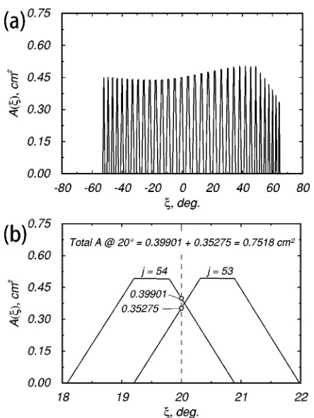
Head 2

Z_start= − 0.918 75 + 0.025B, FIG. 4. Projected area关i.e., expression共18兲兴vs␰for␾= 0° and a start-byte

value of 7 in head 2.共a兲Curves for every fourth stop byte from 0 to 128 have been over plotted.共b兲A zoomed in view for stop bytes 53 and 54 only. Note that constant, flat-topped plateaus occur in the shadow area, As, vs␰ profiles whenever the parallel-projected start-byte aperture and the stop-byte “detector” area have different sizes. This combined with the trigonometric factors in expression共18兲give rise to the variability in the upper envelope in

Zstop= − 6.5535 + 0.072 148B − 2.7909e − 4 B2

+ 5.9784e − 7 B3.

Head 3

Zstart= − 0.918 75 + 0.025B,

Zstop= − 6.3115 + 0.068 3195B − 2.480 15e − 4 B2

+ 5.453 35e − 7 B3.

For the purposes of deriving byte-to-position mappings, the calibration data for head 3 were not usable due to hard-ware problems at the time of calibration. Although in the future, we may be able to recover some additional informa-tion from the calibrainforma-tion data and/or utilize on-orbit data acquired from all three heads to place constraints on the head 3 mappings, this is a complicated task and is beyond the scope of the present article. Therefore, for our present pur-poses, the stop-byte-to-position polynomial for head 3 was derived by averaging the coefficients from heads 1 and 2.

The above polynomials were initially used to derive the start/stop byte-to-angle mappings for both the on-board and statistics data. They are still used for the on-board data, but for the statistics processing we have adopted new angle look up tables 共LUTs兲 that were re-derived from the calibration data in a different manner.

Figure 4 illustrates the projected area obtained for a start byte of 7 in head 2 at␾= 0°. In Fig. 4共a兲, the projected area for every fourth stop byte is over plotted while Fig. 4共b兲 shows more detail for only stop bytes 53 and 54共which peak near␰= + 20°兲.

IV. COLLIMATOR TRANSMISSION PROBABILITY

In the previous section, we computed the directional re-sponse function for a two-element detector comprised of a single narrow start-byte aperture and a single narrow stop-byte detector. This would be sufficient for the MENA instru-ment if there were no collimator, no transmission gratings and no grating support structures. In reality, particles must get through all of those additional apertures before they reach the “start-byte aperture” on the foil. In order to deal with this further complication, we introduce a transmission

function that specifies, for a given direction, the probability

that a particle will reach the foil.

In this section we examine the types of collimating

structures found in the IMAGE/MENA collimator/

transmission grating assembly and we determine, analyti-cally, the separate transmission probability functions associ-ated with each. These probability transmission functions are then combined together in order to obtain the overall trans-mission probability.

A. Collimating structures in MENA

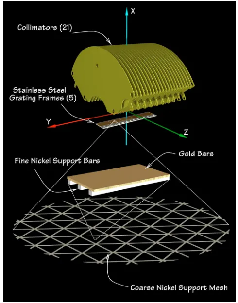
A schematic 3D illustration of the relevant collimating structures in the MENA instrument is given in Fig. 5. Shown in the upper part of the figure are the 21 curved collimator plates and the five stainless steel frames holding the trans-mission gratings. In the lower part of the figure, enlarged views of the coarse triangular nickel support mesh, the fine nickel support bars, and the gold bars of the transmission grating are shown.

The fabrication of the transmission gratings is an ex-tremely difficult process because the gold bars have to be TABLE II. MENA flight unit transmission gratings

Lot No.

Wafer ID

Scribe ID

Frame ID

U04 U04H010 3179 IB037

U02 U02H021 2566 IB057

Head 1 U04 U04H006 3047 IB062

U04 U04H004 3034 IB074

U04 U04H021 3107 IB083

U02 U02H004 2693 IB049

U04 U04H007 3152 IB073

Head 2 U04 U04H003 3151 IB076

U04 U04H001 3158 IB096

U04 U04H002 3188 IB097

U04 U04H007 3152 IB029

U02 U02H004 2693 IB038

Head 3 U04 U04H008 3083 IB075

U04 U04H001 3158 IB089

U04 U04H002 3188 IB100

separated by very small distances 共on the order of 30– 60 nm兲in order to achieve the desired UV-rejection and ion transmission characteristics. As a result of this difficulty, each transmission grating produced for MENA had some-what different rejection/transmission characteristics. In addi-tion, two different “lots” were manufactured for MENA: Lot

U02 and Lot U04. In total, approximately 77 gratings were

mounted in frames for possible use in MENA. To keep track of them all, an inventory numbering system was devised to identify the lot number, the wafer ID and the frame number. After defects were repaired共patching pinholes兲and the UV-rejection and ion transmission characteristics of each grating/frame assembly were measured, 15 were selected for the flight instrument—three from lot U02 and 12 from lot U04. Table II indicates which gratings went into each of the MENA heads.

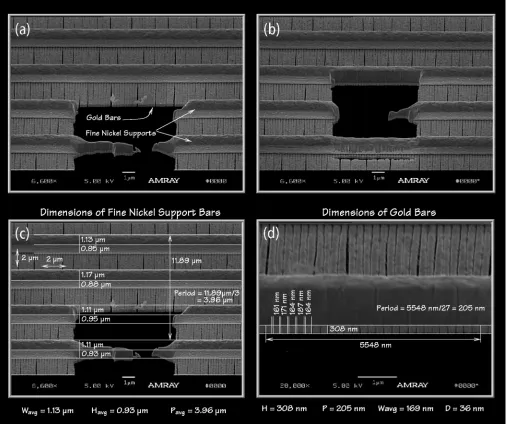
A series of scanning electron micrographs 共SEMs兲of a MENA transmission grating are presented in Fig. 6. The frame ID for this grating assembly is IB030. It comes from

Lot U02 and has wafer and scribe ID numbers of U02H007 and 2994, respectively. Due to a variety of defects, this grat-ing was not considered flight quality. The large rectangular hole in the grating was intentionally cut with an ion beam in order to measure the cross-sectional dimensions of the gold bars and fine nickel support structures.

1. Fine nickel supports

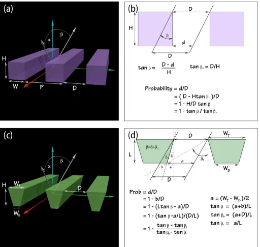
The fine nickel bars that support the gold gratings have either a rectangular or a slightly trapezoidal cross section as shown schematically in Fig. 7. The angle␤is measured from the normal incidence direction perpendicular to the collimat-ing bars while the angle ␣ is measured from the normal incidence direction parallel to the collimating bars. Given the symmetry of the collimating structures, we note that

␶共+␣,␤兲=␶共−␣,␤兲 and␶共␣, +␤兲=␶共␣, −␤兲.

parallel rays共e.g., from a distant source兲impinges on the gap between collimating elements at an angle␤, then only a frac-tion d / D makes it through. Since d = D − H tan␤ and tan␤_ⴰ = D / H共see figure兲, where␤_ⴰ is the maximum angle that can make it through, we have for the transmission probability,

␶= 1 − tan␤/ tan␤_ⴰ.

Note that in terms of the angles ␣ and ␤—which are the angles in the parallel and perpendicular planes, respectively—the transmission probability is independent of

␣.

An additional factor for the overall transmission prob-ability needs to be taken into account: the probprob-ability of actually hitting a gap as opposed to hitting a bar. This prob-ability is just given by ␧= D /共D + W兲, where D is the gap

width and W is the bar 共or plate兲 width. Thus, the overall transmission probability for a collimating structure with rect-angular bars is given by

␶共␣,␤兲=␧

冦

tan␤_ⴰ 兩␤兩⬍␤ⴰ

0 else

冭

, 共19兲

tan␤_ⴰ=D

H, 共20兲

␧= D

共D + W兲. 共21兲

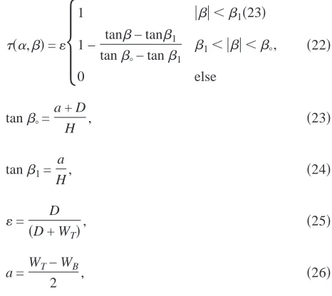
For the trapezoidal geometry, the probability of getting through the structure can be computed as shown in Fig. 7共d兲. Proceeding as above, the overall transmission probability for this collimating structure is given by

␶共␣,␤兲=␧

冦

1 兩␤兩⬍␤1共23兲

1 − tan␤− tan␤1 tan␤_ⴰ− tan␤1

␤1⬍兩␤兩⬍␤ⴰ,

0 else

冧

共22兲

tan␤_ⴰ=a + D

H , 共23兲

tan␤1= a

H, 共24兲

␧= D

共D + WT兲, 共25兲

a =WT− WB

2 , 共26兲

which is again independent of␣.

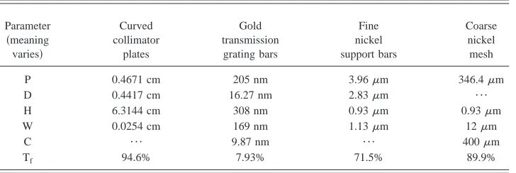
The actual dimensions of the fine nickel support struc-tures were determined from measurements of SEMs as shown in Fig. 6共c兲. Although there is probably a slight trap-ezoidal shape to the fine nickel support bars, the SEMs ana-lyzed so far suggest that the departure from a rectangular geometry is very small. Thus, assuming the nickel bars are rectangular in cross section, the dimensions obtained from Fig. 6共d兲indicate that average bar width, height and period are 1.13, 0.93, and 3.96␮m, respectively.

2. Curved collimator plates

The large curved collimator plates on MENA共i.e., the brass-colored plates shown at the top of Fig. 5兲 can be thought of as very narrow and tall rectangular bars that are curved into arc shapes. The above transmission probability for the rectangular geometry is still valid for this case if we note that the height of each bar decreases by a factor of cos␣. Thus, for the curved collimators, the transmission probability is dependent on ␣ because the value of ␤_ⴰ in-creases as␣ increases.

3. Gold grating bars

Although the gold grating bars were intended to have a rectangular geometry, technical limitations in their fabrica-tion lead to bars that have a more “barrel-shaped” geometry. By this we mean that the cross section of each bar is like a rectangle with “bulging” sides 共i.e., each bar looks like a barrel when viewed edge on兲. Here we develop an analytic expression for the transmission function associated with such structures under the assumption that the bulging sides can be expressed as arcs of circles.

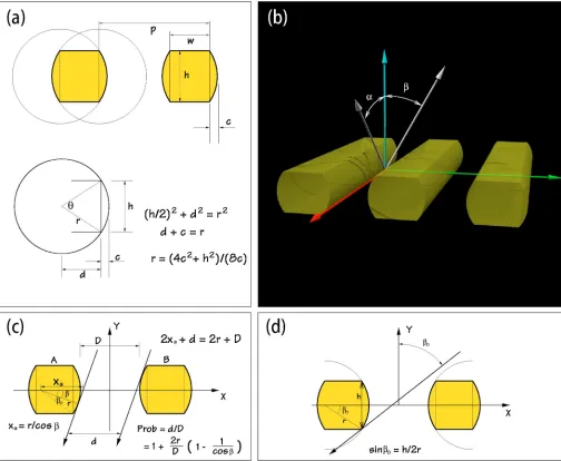
The barrel geometry can be approximated by the inter-section of a rectangular bar and two cylinders as shown in Figs. 8共a兲and 8共b兲. From the lower part of panel共a兲, we can see what the radius of each circle needs to be, given that we

know the height h of a bar and the distance c that the middle of the bar sticks out relative to the tops and bottoms of the bar

r =h 2_{+ 4c}2

8c . 共27兲

If the gap between two bars is given by D, and we place the origin at the center of the gap, then the circle defining the left side of the gap is centered at a point −共D / 2 + r兲, while the circle defining the right side of the gap is centered at a point +共D / 2 + r兲.

As shown in Fig. 8共c兲, the transmission probability,␶, is given by the quantity d / D, where D is the 共known兲 gap width and the distance d is a function of the angle␤. Note that, as with the rectangular and trapezoidal geometries dis-cussed above, since␤ is defined as the angle between the y axis and the projection of the ray onto the x-y plane, the transmission probability will be independent of the angle␣ 共which is defined as the angle between the y axis and the projection of the ray onto the y-z plane兲.

In order to compute the transmission probability for this type of collimating structure, we note that there are three distinct cases to consider. The first case occurs when the incident rays enter the gap such that they are tangent to the cylindrical portions of the barrels. This will occur when兩␤兩

⬍␤0. The second case occurs when ␤0⬍兩␤兩⬍␤1. In this

case the incident rays are tangent to the cylinders at points that are not on the defined barrel. In this regime, d is calcu-lated simply by considering the corner points as we did for the rectangular geometry. Finally, the third case occurs when 兩␤兩⬎␤1. For this case no rays can get through and the

prob-ability must be 0.

From Fig. 8共d兲, we can see that the limiting angles are given by

sin␤0= h/2r, 共28兲

tan␤1=共2c + D兲/h. 共29兲

Also, from Fig. 8共b兲, we see that for 兩␤兩⬍␤0

d = D + 2r

冉

冊

␶= 1 +h

2_{+ 4c}2

4cD

冉

cos␤

冊

When␤0⬍兩␤兩⬍␤1, the transmission probability can be

␶= d/D = 1 +2c

D −

h

Dtan␤. 共30兲

Combining all three cases together we finally have the transmission probability for the gold bars

␶共␤兲=␧

冦

␶1, 兩␤兩⬍␤0

␶2, ␤0⬍兩␤兩⬍␤1

0, 兩␤兩⬎␤1

冧

␶1= 1 +

h2_{+ 4c}2

4cD

冉

cos␤

冊

␶2= 1 +

2c

D − h

Dtan␤

sin␤0= h/2r

tan␤1=

共D + 2c兲

h 共31兲

␧= D

D + w.

The dimensions of the gold bars present in grating IB030 共from lot U02兲were measured from the SEM shown in Fig. 6共d兲. The average height, width, period and gap size were determined to be 308, 169, 205, and 36 nm, respectively.

4. Coarse nickel supports

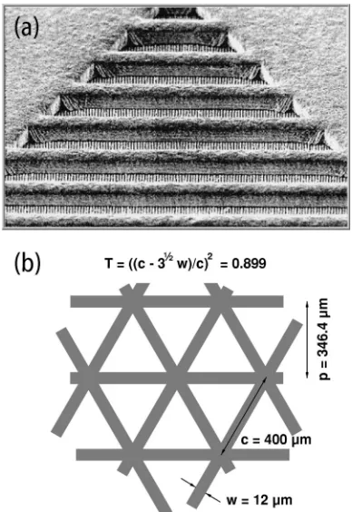
The coarse triangular nickel support mesh is a much more macroscopic structure than either the fine nickel sup-port bars or the gold grating bars. In addition, as shown in the scanning electron micrograph in Fig. 9共a兲, it lies in the same layer and has the same height as the fine nickel support bars. As a result, the modification of the overall angular de-pendence of the transmission characteristics due to the coarse mesh will be very small. Thus, for the coarse triangular mesh we assume a uniform constant transmission factor of 0.899. This value is derived from the dimensions shown in Fig. 9共b兲.

B. Overall transmission efficiency

1. Collimating structures

The transmission functions for the curved collimator plates, the gold bars, and the fine nickel support bars in terms of the coordinate system defined in Fig. 2共a兲are given by

␶C共␰,␾兲=␧_C

冦

兩␾兩⬍␾ⴰ,C

0 else

冧

␶TG共␾兲=␧TG

冦

␶1, 兩␾兩⬍␾0,TG

␶2, ␾0,TG⬍兩␾兩⬍␾1,TG

0, 兩␾兩⬎␾1,TG

冧

␶NS共␰兲=␧NS

冦

1 兩␰兩⬍␰1

1 − tan␰− tan␰1 tan␰_ⴰ− tan␰1

␰1⬍兩␰兩⬍␰_ⴰ

0 else

冧

␶CM= 0.899

␶1= 1 +

h2+ 4c2

4cD

冉

cos␾

冊

␶2= 1 +

2c

D − h

Dtan␾

tan␾_ⴰ,C= DC

HCcos␰ sin␾_0,TG= H_TG/2r tan␾1,TG=

共DTG+ 2c兲 HTG

tan␰_ⴰ=共aNS+ DNS兲

HNS

tan␰1= aNS H_NS

aNS=

WT− WB

2

␧C=

冉

D_C

DC+ WC

冊

␧TG=

冉

DTG+ WTG

冊

冉

DNS

DNS+ WT,NS

冊

The subscripts C, TG, NS, and CM refer to the Collima-tor, Transmission Grating, Nickel Support, and Coarse Mesh structures, respectively. Note that we have left these terms as functions of␰ and␾for clarity. It is a simple task to make them functions of␪ and␾instead.

2. Energy dependence

Since all atoms with energies above about 1 keV are able to make it through the foil, the transmission efficiency above 1 keV is taken to be 100%. Below 1 keV the trans-mission efficiency will begin to drop due to the finite thick-ness of the carbon foil. In this regime, the efficiency will also be dependent upon the angle of incidence since the path length through the foil is dependent upon the angle of inci-dence. A detailed calculation of these efficiencies can be made using theTRIMcode,5but for our present purposes we will simply restrict our analysis to energies above 1 keV and assume 共to a good approximation兲 that there is no energy dependence to the transmission efficiency.

3. Postfoil detection efficiency

For ENAs that make it through the collimator, transmis-sion grating and foil, an additional postfoil detection effi-ciency must be taken into account. This additional effieffi-ciency results from a number of individual efficiencies including: the probability of generating secondary electrons in the foil; the probability of detecting the primary ENA; the probability of detecting the secondary start electrons; and the probability of making it through the accelerating and shields grids. Al-though this combined efficiency is not easy to compute from first principles, it can be measured in a relatively simple FIG. 9.共a兲SEM showing a corner region of the coarse nickel mesh. The

manner in the laboratory using a combination of the coinci-dence and singles rates from the start and stop portions of the detector.

If ENAs are passing through the foil at a rate S and at an angle of incidence such that the parallel-projected area of the entrance aperture falls completely within the active area of the stop detector, then the individual singles rates in the start and stop detectors will be given by: RA=␧AS and RB=␧BS, respectively. Furthermore, if the detectors are independent, the coincidence rate will be: RAB=␧A␧BS + Rch=␧S + Rch

where the overall postfoil detection efficiency,␧, is equal to

␧A␧B. Here, Rchis the chance coincidence rate which is

ap-proximately given by TR_AR_B, where T is the coincidence time window. In our case, the overall postfoil efficiency is near 40% and the laboratory measurements were taken with singles rates on the order of 1 kHz and a time window of approximately 300 ns. Therefore 共in the laboratory兲, Rch is

negligible in comparison to the total measured coincidence rate, RAB, and can be safely neglected.

Since S = RAB/␧, we have ␧A␧B=共␧RA/ RAB兲

⫻共␧RB/ RAB兲=␧. Thus

␧=共RAB兲

2

RARB

. 共32兲

Use of this formula together with measurements of the coin-cidence and singles rates taken in the laboratory prior to launch gives a total overall postfoil detection efficiency of

␧= 0.424.

4. Overall detection efficiency

Finally, a total transmission probability as a function of look direction can be defined as the product of all the rel-evant probabilities

␶共␪,␾兲=␶C共␾兲⫻␶TG共␪,␾兲⫻␶NS共␪,␾兲␶CM⫻ ␧. 共33兲

The various dimensions assumed for the three collimating structures are summarized in Table III and plots showing the dependence of␶C,␶TG,␶NS, and␶on the angles␣and␾are

shown in Fig. 10.

V. GEOMETRIC FACTORS

For each start and stop-byte combination, we can define a geometric factor as follows:

Gijk=

冕

␪=−␲/2 +␲/2

冕

Aijk共␪,␾兲␶共␪,␾兲cos␪ d␪d␾. 共34兲 Here, i and j correspond to start- and stop-byte numbers and

k corresponds to the head number共0, 1, or 2兲.

The G_ijk for IMAGE/MENA were computed 共 numeri-cally兲 and are shown in Fig. 11. Note that there is a very significant degree of asymmetry in each head and that the three heads are all different. The anomalously low ampli-tudes for start bytes 4 and 14 are due to the fact that those start bytes correspond to physical entrance apertures at the edges of the grating and are therefore chopped to smaller sizes than those start bytes that map to the central regions of the grating. Similarly, start bytes关0–3, 15兴all map to regions outside of the entrance aperture and therefore they all have

G⬅0.

VI. CULLING OF DIRECT EVENTS

For the sake of simplicity, we have so far ignored the fact that each head actually has a central blind spot. This blind spot exists because the section of the detector area below the start foil must be dedicated to detecting start elec-trons and cannot simultaneously detect ENAs. Therefore, in reality, the geometric factors for each start byte will drop very rapidly to zero for stop-byte values that map to the start section of the position sensitive detector. The exact stop-byte ranges where the count rates first begin to drop for each start byte can be easily determined from the data itself. We have compiled these values into a “mask” array which we use to “cull out” start/stop-byte pairs that map within or close to the edges of the central blind spot. This simple approach allows us to use the geometric factors shown in Fig. 11 without modification since the nonphysical regions will never be used.关Note that the specific start/stop-byte pairs that we cull can be seen as black areas in the angle look up tables共LUTs兲 shown later in Fig. 12共a兲.兴

VII. COMPARISON WITH ABSOLUTE CALIBRATION

The effective area at various incident angles for heads 1 and 2 in the MENA instrument were measured in the labo-ratory prior to launch. A broad beam source of H+_{and O}+_at

31 keV and of H+_{at 9 keV were used for this purpose. The}

beam was broad enough to fill the entrance aperture and was measured to have very low divergence共⬇0.1°兲so that, to a very good approximation, it can be considered as a parallel-TABLE III. MENA collimator dimensions and transmission efficiencies.

Parameter

共meaning varies兲

Curved collimator plates Gold transmission grating bars Fine nickel support bars Coarse nickel mesh

P 0.4671 cm 205 nm 3.96␮m 346.4␮m

D 0.4417 cm 16.27 nm 2.83␮m ¯

H 6.3144 cm 308 nm 0.93␮m 0.93␮m

W 0.0254 cm 169 nm 1.13␮m 12␮m

C ¯ 9.87 nm ¯ 400␮m

ray source. The beam was also imaged with a two-dimensional共2D兲imager in order to verify that it was spa-tially uniform to a high degree. The omni-directional flux J of the beam共in units of number/ cm2/ s兲was measured with a Faraday cup detector. The beam was then directed into the MENA instrument heads at various angles of incidence in order to determine the total coincidence共or “valids”兲rate, C. The effective area of a head at a given angle of incidence can then be calculated as Aeff= C / J. As discussed elsewhere, the

results for head 3 are unreliable. This is because the 1 keV foil bias voltage cable separated from the instrument during calibration runs. However, the data for heads 1 and 2 give effective areas as follows:

A_1,eff= 0.10 ± 0.04 cm2,

A2,eff= 0.11 ± 0.06 cm2.

coincidence 共or valids兲 rate, for a given start byte, and a given incident angle, we can consider the projected area as the sum of all the projected areas obtained from each stop

along with the overall transmission efficiency at␪= 20° and the resulting effective area. The “stop-bytes” column indi-cates which stop bytes actually contributed to the sum共for

␪= 20°兲. Summing the effective areas for each start byte gives a total effective area at␪= 20° of

A_2,eff= 0.1353 cm2. 共35兲

Note from Table IV that the total projected area is 7.5175 cm2 which is just the total area of the gratings 共5⫻1.0 cm⫻1.6 cm= 8.0 cm2兲 multiplied by cos共20°兲. We could have guessed this from the outset, but the above analy-sis provides an excellent check on our calculations of the byte-dependent projected area curves 共like those shown in Fig. 4兲.

Although there is considerable uncertainty in the mea-surements for the effective area, our calculated value for head 2 is reasonably close to the measured value of 0.11± 0.06 cm2 and is well within the uncertainty range.

VIII. INTEGRAL FLUX IMAGES

From Eq. 共5兲, the count rate for a given start byte 共i index兲, stop byte共j index兲, head ID共k index兲, and azimuth bin共ᐉindex兲is given by

C_ijkᐉ=

冕

j_0,ijkᐉ共E兲⌫ijk共E兲dE. 共36兲

Since the angular distribution of the differential flux does not vary much over a start-byte/stop-byte pair, we can safely set

F共␪,␾兲= 1 so that⌫ijk共E兲= Gijk共E兲. Furthermore, if the over-all detection efficiency is independent of energy共for energies above about 1 keV this is a good approximation兲, then

Gijk共E兲= Gijk. We then have

Cijkᐉ= Gijk

冕

j0,ijkᐉ共E兲dE. 共37兲

To define an “integral flux,” Jijkl, we accumulate counts from a given lower cutoff energy, Eo, up to E =⬁. Then

Cijkᐉ= Gijk

冕

⬁

j0,ijkᐉ共E兲dE = GijkJijkᐉ. 共38兲

The integral flux, J, is therefore given by

J_ijkᐉ=Cijkᐉ

G_ijk. 共39兲

To perform this calculation for the IMAGE/MENA direct-events data, for each head and azimuth bin, counts are first accumulated into stop-byte/start-byte bins. Then the to-tal count rate for that bin, Cijkᐉ, is divided by the correspond-ing geometric factor, Gijk. Each of the resulting integral fluxes are then mapped to the polar angle implied by their ijk values. The interactive graphical tool shown in Fig. 12共a兲 illustrates this process step by step. The top three rows show the process for heads 1, 2, and 3 separately, while the bottom row shows all three heads combined. From left to right the top three rows show:共1兲the polar angle look up table共LUT兲 as a function of start共horizontal dimension兲and stop 共 verti-cal dimension兲bytes;共2兲the raw total count rate as a func-tion of stop byte for start bytes of 0–15 共i.e., there are in essence 16 curves of count rate versus stop byte overplotted兲; 共3兲the raw total count rate as a function of polar angle共each bin’s start and stop byte gives a polar angle via the angle LUTs兲;共4兲integral flux共count rate divided by G兲as a func-tion of polar angle; 共5兲 integral flux binned into 4° polar angle bins;共6兲complete all-sky image for a given head with azimuth angle on the vertical axis and the polar angle on the horizontal axis.

All of the line plots are averaged over the azimuthal bins indicated by the yellow bar that appears to the right of each all-sky image. For the top three rows, the polar angle plots range from −60° to 60° and are all in the “head frame”共in which ␪= 0° is perpendicular to the detector plane兲. In the bottom row, the individual heads are combined by shifting heads 1 and 3 by ±20° with respect to head 2. In addition, the plots that are functions of polar angle range from −80° to 80° in the bottom row. To reduce artifacts in the final merged image, note that we do not simply merge together the three individual head images. Instead, we bin the combined cor-rected angular distributions共i.e., the processing always flows from left to right in Fig. 12共a兲—not top to bottom兲.

Although the geometric factors obtained do an excellent job of converting counts to flux, combining data from the three heads together almost always produces artifacts in the final image if additional processing is not performed. The two main reasons for this are: 共1兲 the overall relative effi-ciencies of the three heads may vary to some degree, and共2兲 there may be different amounts of background noise in each image. In addition, the background noise must be subtracted from the count rate, not the final fluxes. In the presence of background noise and an overall efficiency factor, the flux is given by

J =␧

冉

G

冊

In order to seamlessly merge data from the the three separate heads together, we first need to determine the rela-tive efficiencies and the background count rates. Since we TABLE IV. Calculated effective areas at␪= 20° for head 2.

Start byte Stop bytes

Projected area

cm2 _␶

Effective area cm2

0 ¯ 0.000 00 0.017 99 0.000 00

1 ¯ 0.000 00 0.017 99 0.000 00

2 ¯ 0.000 00 0.017 99 0.000 00

3 ¯ 0.000 00 0.017 99 0.000 00

4 49–50 0.610 80 0.017 99 0.010 99

5 50–51 0.751 75 0.017 99 0.013 53

6 51–53 0.751 75 0.017 99 0.013 53

7 53–54 0.751 75 0.017 99 0.013 53

8 54–56 0.751 75 0.017 99 0.013 53

9 56–57 0.751 75 0.017 99 0.013 53

10 57–59 0.751 75 0.017 99 0.013 53

11 59–61 0.751 75 0.017 99 0.013 53

12 61–62 0.751 75 0.017 99 0.013 53

13 62–64 0.751 75 0.017 99 0.013 53

14 64–64 0.140 95 0.017 99 0.002 54

15 ¯ 0.000 00 0.017 99 0.000 00

are only interested in relative efficiencies for this operation, we peg the overall efficiency of head 2 as␧₂⬅1 and let the efficiencies of heads 1 and 3共␧₁and␧₃兲as well as the back-ground count rates in all three heads共B₁, B₂, and B₃兲vary as free parameters. We determine the five unknown parameters using a fitting procedure to minimize the total absolute dif-ference共in log space兲between the fluxes that result at polar angles where the three heads overlap. The problem is not under determined since there are five unknowns and five re-gions of overlap. More work needs to be done on which azimuth bins should be used for this fitting procedure, but the results so far are quite encouraging. In addition, strong emis-sions tend to dominate the fit which can sometimes produce obvious artifacts in very low flux regions. For this reason, we tentatively chose to fix the background rates at 0.0 in Fig. 12. A projected version of the final integral flux image shown in Fig. 12共a兲is presented in Fig. 12共b兲. The data are shown in a 360° fish-eye projection looking toward the cen-ter of the earth. Gaps in coverage near the poles of the all-sky image 共polar angles approaching ±90°兲 can be seen as distorted black circular regions to the left and right of the earth. The broad black horizontal gap connecting the poles corresponds to azimuth bins for which the instrument auto-matically turned off during its sweep past the sun. The bright regions above the sun gap are likely spurious counts due to solar UV photons. The grid seen through the data is the

un-derlying equatorial plane of the solar-magnetic共SM兲 coordi-nate system and the lines are drawn every 2 R_Ein both the x and y directions. The bright 共yellow, orange and red兲 emis-sions are ENAs emitted from regions quite close to the earth, while the more extended dimmer emissions 共blue to cyan兲 are emitted farther out from the plasma sheet. Note that in this somewhat peculiar projection, the inner part of the im-age共i.e., the circular region inside of the poles兲corresponds to the more familiar 180° fish-eye projection, while the ring outside of this corresponds to regions that are actually “behind us.” While the mapping in the outer regions is not intuitively obvious 共especially near the poles兲, this type of projection allows us to display/monitor all of the data avail-able at once without adversely distorting the view in the earthward direction.

In Fig. 13, the count rate versus angle and the integral flux versus angle panels are shown enlarged for six different events. The contributions from each head are color coded: head 1 is green; head 2 is yellow; and head 3 is blue. As can be seen, in all cases the head-to-head match is excellent.

IX. DIFFERENTIAL FLUX IMAGES

As in the previous section, the count rate for a given start byte 共i index兲, stop byte 共j index兲, head ID 共k index兲, and azimuth bin共ᐉ index兲is given by

C_ijkᐉ=

冕

j_0,ijkᐉ共E兲Gijk共E兲dE. 共41兲

If j0,ijkᐉ共E兲and Gijk共E兲do not change much over the range of

integration共e.g., spectrum is flat or⌬E is small兲, this expres-sion can be approximated by

Cijkᐉ= Gijkj0,ijkᐉ共E兲⌬E. 共42兲

Thus

j0,ijkᐉ共E兲= Cijkᐉ

Gijk共E兲⌬E. 共43兲

Technically, this equation is correct, but as we shall see in the next section its naive application leads to several prob-lems.

A. Problems with energy binning

In order to determine the energy of a particle in the MENA instrument, we need to know: its time of flight 共TOF兲; its angle of incidence; and its mass. If we assume for the moment that all of the ENAs are hydrogen, then we can ignore the mass dependence. Then, the angle of incidence gives the path length, the TOF and path length give the speed, and the speed and assumed mass give the energy. The

main problem with this scheme arises as a result of two separate effects:共1兲once measured, the TOF value is digi-tized into fairly coarse “TOF bytes” and共2兲the mapping of TOF byte to energy changes as a function of polar angle 共because the path length changes兲.

These effects are illustrated in Fig. 14. The image in the lower left portion of the figure is an integral flux image from head 2 and the two vertical arrays represent the 64 TOF byte values possible in the direct events data. The array on the left shows the TOF to energy mapping for a pixel at a polar angle of −40° while the array on the right shows the TOF to energy mapping for a pixel at a polar angle of −28°. As can be seen, the midpoint energy for each TOF byte is somewhat different for the two pixels. The main effect of this variation is that for a given requested energy band, a different set of TOF bytes will end up getting used depending on what angle we are looking at. For example, if we ask for energies between 2 and 5 keV, the TOF bytes that will be used at −40° and −28° are those that are shaded green in Fig. 14. The right-hand side of Fig. 14 shows the TOF bytes that would be used for other requested energy bands at the midpoint of the nominal 4° polar angle bins共note that we are not restricted to using 4° bins兲.

At this point, it is important to recognize that the⌬E that

appears in Eq.共43兲 is not the one explicitly defined by the requested energy band. Rather it is the one implicitly implied by the specific grouping of TOF bytes that actually get used at each polar angle. This is a serious problem because it means that both⌬E and E vary with polar angle. To illustrate

this more clearly, we plot⌬E 共purple points兲 and E 共green points兲as a function of polar angle in Fig. 15 together with the raw count rate共white points兲as a function of␪. In this plot we have not binned the data into regular polar angle bins which is why there are so many different angles represented. While the variation of E and ⌬E is apparent in each

panel, the most obvious and disturbing feature of this plot is that for all but the 1 – 1000 keV requested energy band, E and⌬E are in fact discontinuous functions of polar angle.

The effect these discontinuities have on the raw count rate is

clearly visible. Note that, even for a requested energy band of 1 – 60 keV, small but very noticeable discontinuities ap-pear in the count rate data. These artifacts get much more severe for the higher energy bands and/or when the requested

⌬E gets smaller共i.e., when⌬E / E gets small兲. Another arti-fact that is introduced when⌬E / E becomes too small is that

gaps begin to appear in polar angle coverage as shown in the 20– 25 keV panel. This occurs because⌬E gets so small that

none of the TOF-byte midpoint energies fall in the requested energy range for some polar angle ranges.

B. Solution to energy binning problems

divide by the appropriate value of⌬E. The reason this does

not work is that while it formally results in a proper differ-ential flux, the energy, E, at which the differdiffer-ential flux is evaluated for still changes discontinuously as a function of polar angle. In other words, dividing by the proper⌬E

pro-duces differential flux images where each polar angle repre-sents a different energy. In addition, this approach does noth-ing to avoid the introduction of gaps in polar angle. Clearly, in order to be able to generate uniform-energy differential flux images at arbitrary energies, a different approach is nec-essary. In this section we describe an alternative processing scheme that overcomes these problems and is also reason-ably simple to implement.

Rather than trying to bin the data into pre-selected en-ergy bands共e.g., 1 – 2 keV, 2 – 5 keV, etc.兲, we instead con-struct a “differential flux versus energy spectrum” for each pixel in the final image. Once this is done, the differential flux at any desired energy can be interpolated from these spectra. This approach ensures that the fluxes in each of the pixels in the final image will be evaluated at the same energy and it also eliminates the gaps that were described in the previous section. The task of creating differential flux images therefore boils down to three distinct subproblems:共1兲 Cal-culation of the differential flux energy spectrum for a given pixel in a given head;共2兲combining the spectra together in pixels where heads overlap, and;共3兲interpolating to the de-sired energy.

1. Differential flux energy spectra From Eq.共43兲, we can write

j0,ijk_ᐉt共Eijkt兲=

Cijk_ᐉt

Gijk共Eijkt兲⌬Eijkt

共44兲

= Cijkᐉt

Fijk共Eijkt兲, 共45兲

where, Fijk共Eijkt兲 is the “flux conversion factor” 共FCF兲, i is the start-byte index, j is the stop-byte index, k is the head ID,

ᐉis the azimuth bin number, and t is the TOF-byte index. As we have noted above, this simple formula can be used to convert raw count rate to flux provided that the true flux j and the geometric factor G do not change very much over the range of energies considered,⌬E. In our case this is a

rea-sonable approximation since G is approximately independent of energy above 1 keV and each TOF byte implies a fairly narrow “energy aperture.”

Our algorithm for computing the differential flux versus energy spectrum in a single pixel for a single head is outlined below.

• Define the polar angle pixels. Nominally these will be 4° or 5° wide, but for a given head they can be any reasonably small value. However, in order to properly merge the final spectra for each head together into a single image, we should restrict the polar angle bin size to values that are multiplicative factors of 20°.

• For a given pixel, scan through the raw direct events and select those that contribute to the pixel, i.e., select

those events that have start/stop/azimuth byte combina-tions that fall in the ⌬␪/⌬␾ range implied by the se-lected pixel.

• Convert each selected event to a differential flux using the appropriate geometric factor, Gijk, and the ⌬E im-plied by its TOF-byte value. Also keep track of all the corresponding energies that result from this operation. At this point we technically have a differential flux ver-sus energy spectrum in the pixel. However, in practice the counting statistics will be extremely poor if we stop here.

• To build up counting statistics, we bin the differential fluxes into a smaller number of discrete TOF bins. One way to accomplish this is to average the fluxes into 64 bins according to their TOF values. The energy that we associate with each bin is then taken to be the average energy of the fluxes that went into that bin. Since there are many TOF bins at the lower energies, each with very narrow ⌬E ranges, the counting statistics at low

energies can still be quite poor. Thus an alternate bin-ning scheme in which groups of low-energy TOF bins are averaged together can be used instead. The latter binning scheme generally yields better results.

2. Combining spectra from different heads

Once the differential flux versus energy spectrum has been determined for each pixel in all three heads, we are ready to combine the three heads together. In pixels of the final image where two heads overlap共note that there are no pixels for which three heads ever overlap兲, the two different energy spectra must be merged together. One way to accom-plish this is to simply create a new merged spectrum from the flux versus energy data points in each head 共this will result in a merged spectrum with twice the data points con-tained in a single head spectrum兲. A negative aspect of this approach is that it often introduces artifacts into the final image because the spectrum from one head may have much poorer counting statistics than the other. In order to solve this problem, we use a weighted average of the individual spectra instead of just merging the data points. The weights are de-termined by the number of counts that went into each flux estimate.

3. Interpolating to the desired energy

After the energy spectrum for a given pixel has been computed, the differential flux at a given energy is obtained by interpolation共or extrapolation if necessary兲. Several inter-polation methods have been implemented including: linear interpolation; B-spline interpolation, Cardinal spline interpo-lation共joined Bezier spline segments in which only zeroeth and first order derivatives are forced to be continuous兲; ro-bust straight line fitting of nearby points共with an adjustable number of points in the fit兲; Maxwellian distribution fit; and a Kappa distribution6 fit.

the interpolated curve always lies in the “convex hull” of the piece-wise linear curve defined by the control points.7Thus, the curve is not forced to go through any of the data points and will never “blow up.”

An interactive graphical tool illustrating the steps out-lined above is shown in Fig. 16. From left to right and top to bottom, the six panels containing line plots show: Counts versus TOF byte; counts/G versus TOF byte; differential flux versus TOF byte; differential flux versus re-binned TOF bins; differential flux versus energy; differential flux versus energy from re-binned TOF bins. The four panels on the right show the differential flux images obtained from each head plus the combined image. The line plots correspond to the pixel marked with a cross hair. The differential flux images were evaluated at 5 keV and the interpolated value for the pixel under the cross hair is shown as a larger orange square in the lower-right line plot. The vertical lines on the lower two plots are drawn at energies of 共1, 2, 5, 12, 27, 40, and 60 keV兲.

The data shown in Fig. 16 were acquired on orbit by

MENA over an accumulation time of 420 min between 17 and 24 UT on October 4, 2000. Although for routine scien-tific analysis we would not consider using such long integra-tion times, here it is useful to monitor the effects of our processing without the counting noise obscuring the results. Although a few artifacts remain in the final differential flux image共in the form of vertical stripes兲, the overall quality of the image is quite high. An additional feature that can be seen in the energy spectra for these long-time-average im-ages is the possible presence of two distinct particle popula-tions. This can be seen in the differential flux versus energy plot shown in the lower left hand panel of Fig. 16. It is quite possible that the component appearing at lower energies could be due to oxygen ENAs, although more work needs to be done in order to verify this hypothesis.

from the northern hemisphere共r_GSM= 3.0, 0.6, 7.5RE兲looking down toward the center of the earth which is located at the center of each image. The sun共i.e., local magnetic noon兲is roughly toward the top共closer to “11 o’clock” position兲of each image and local magnetic midnight is roughly toward the bottom共closer to “5 o’clock position”兲. A magnetic storm was under way during this event and the images reveal a somewhat unusual morphology in which the ring current peaks on the day side. This is consistent with data acquired by the higher-energy ENA imager 共HENA兲 on the IMAGE spacecraft.8

X. OUTSTANDING ISSUES AND FUTURE WORK

In the previous sections we discussed processing algo-rithms that we have developed for creating both integral and differential flux images from the raw MENA direct events data and the example shown in Fig. 17共a兲 clearly demon-strates the effectiveness of our approach. Nevertheless, sev-eral outstanding issues remain that we still need to address and we will briefly discuss them below.

A. Scattering, point spread function, and image deconvolution

In our calculation of the geometric factors above, we assumed that ENAs incident on the start foil关see Fig. 1共d兲兴 pass through it unperturbed on straight-line trajectories. In reality, the thin carbon foils used in the MENA instrument can produce a significant degree of angular scattering of the incident ENAs. As discussed by Funsten, McComas, and Barraclough,9 the scattering half angle is inversely propor-tional to the incident particle energy

␺1/2= kF

E, 共46兲

where the “foil constant,” kFdepends on the incident particle type 共e.g., H or O兲, the target composition 共carbon in our case兲, and the thickness of the foil 共for MENA, the carbon foils have a mass per area value of approximately 1.1␮g / cm2giving a thickness of⬇49 Å兲.

lighter ones do共i.e., H兲. In order to remove this undesirable effect, the “scattering function” must be deconvolved from the images in the head frame. Although simple Fourier meth-ods for image deconvolution exist,10it is important to recog-nize that they do not work well in deconvolving extended sources and they also rarely yield acceptable results in situ-ations where there is significant noise present. Several de-convolution methods that are more suitable for our purposes are discussed in Jansson’s book11and in a review article by Starck, Pantin, and Murtagh.12 The so-called “Damped Richardson-Lucy” algorithm is a particularly appealing can-didate because: it is explicitly based on a maximum-likelihood solution for Poisson statistics; it “conserves en-ergy;” it ensures “positivity;” it is iterative and therefore fast; and it is specifically designed to work with extended sources. We have implemented the method and applied it to the final images with some encouraging initial results 共but we note that a proper implementation requires the deconvolution to be done in the head frame, not the final image frame兲.

B. Point spread function and polar-angle “blooming” artifacts

Perhaps the most obvious and unnatural artifact in the MENA images is the “polar angle blooming” effect as illus-trated in Fig. 17共b兲. It seems to occur when MENA is imag-ing particularly intense low-altitude emissions from near the limb of the earth at relatively oblique viewing angles 共i.e., when IMAGE is not high above the pole兲. Under these con-ditions, the azimuth bins affected共usually only one or two of them兲show a broad enhancement over an anomalously wide range of polar angles. This feature is indicated by an arrow in Fig. 17共b兲. Our initial, tentative interpretation of this feature is that it could be a result of the low-altitude ENA emissions having a significant oxygen content. Since oxygen neutral atoms共at a given energy per amu兲will undergo substantially more scattering in the thin carbon foil 共e.g., see Funsten, McComas, and Barraclough9兲, the signal would “spread out” more in the imaging 共polar-angle兲 direction. Note that this implies that the point spread function in the polar angle di-rection is likely to be species dependent as we mentioned in the previous section.

C. Sun signal contamination

Although the nano-structure transmission grating used in the IMAGE/MENA heads was designed to reject UV pho-tons 共while at the same time transmitting ENAs兲, the IMAGE/MENA instrument still turns off once each 2 min spin period as it sweeps past the sun in order to avoid dam-age to the detectors from the very intense flux of solar UV photons. Despite this safeguard, we have discovered that the MENA instrument still appears to respond to solar photons— and in certain circumstances the peak response can occur when the instrument is not even looking directly at the sun. In order to determine the source of this contamination, we have computed the total projected共or “effective”兲area of solar-illuminated surfaces upstream of the gratings共 collima-tor plates and inner surfaces of the collimacollima-tor housing struc-ture兲 as a function of spin phase angle. We find that this

projected area is highly correlated with the polar-angle-summed count rate versus spin phase. We therefore surmise that the anomalous sun signal present in the data is due to reflection of solar UV photons from the collimator plates and from the collimator housing structure into the detector.

A detailed calculation of these effects from first prin-ciples would be extremely difficult and is far beyond the scope of the present article. Although more work needs to be done in modeling the photon response, the removal of this artifact from the images will almost certainly be accom-plished with an ad hoc empirical processing scheme.

D. Correct background subtraction

In counting experiments, the number of counts observed typically obeys a Poisson distribution. If we have an under-lying count rate, r, and an observing time, T, then the ob-served number of counts, n, will be Poisson-distributed as follows:

p共n兩r兲=共rT兲 n

n! e

−rT_{. 共47兲}

Here, p共n兩r兲is the probability of getting n counts given that we know that the rate has a value r. However, our problem is quite different from this one. We wish to infer the value of r, given that we observed n counts in the共known兲time interval,

T. In other words, what we need to compute is p共r兩n兲. This can be accomplished by using Bayes’ theorem which gives 共e.g., see Loredo13and D’Agostini14兲the “posterior distribu-tion”

p共r兩n兲=T共rT兲 n_e−rT

n! . 共48兲

The mode共most probable value, i.e., the peak of the distri-bution兲, mean 共具r典=兰rp共r兩n兲dr兲, and standard deviation 共具r2_{典−具r典}2_兲1/2 _{of this distribution are: n / T, 共n + 1兲/ T, and}

冑n + 1 / T, respectively. One way to summarize the inferred

value of r is to report the most probable value共the mode兲 together with a “credibility region” containing 95% of the posterior density. The credibility region will in general be asymmetric about the mode and will never contain negative numbers. Note that when n is large, the Poisson distribution can be approximated by a Gaussian with mode, mean, and standard deviation of: n / T, n / T, and

冑n / T, respectively,

Although this result seems trivial 共we would have cho-sen r = n / T even without the Bayesian analysis兲, it does allow a more rigorous treatment of uncertainties and, as we shall see, the Bayesian approach allows us to correctly deal with background subtraction. The following description of correct background subtraction is discussed much more thoroughly in Loredo.13