Munich Personal RePEc Archive
Dynamic Factor analysis of industry
sector default rates and implication for
Portfolio Credit Risk Modelling
Cipollini, Andrea and Missaglia, Giuseppe
University of Essex
30 May 2007
Dynamic Factor analysis of industry sector default rates and
implication for Portfolio Credit Risk Modelling
Andrea Cipollini
aand Giuseppe Missaglia
ba
Corresponding author: University of Essex, Department of Accounting, Finance and Management, Wivenhoe Park, Colchester C04 3SQ, United Kingdom. E-mail: [email protected]
b
BNL Rome, Italy.
30 May 2007
Abstract
In this paper we use a reduced form model for the analysis of Portfolio Credit Risk. For this
purpose, we fit a Dynamic Factor model, DF, to a large dataset of default rates proxies and
macro-variables for Italy. Multi step ahead density and probability forecasts are obtained by employing
both the direct and indirect method of prediction together with stochastic simulation of the DF
model. We, first, find that the direct method is the best performer regarding the out of sample
projection of financial distressful events. In a second stage of the analysis, the direct method of
forecasting through principal components is shown to provide the least sensitive measures of
Portfolio Credit Risk to various multifactor model specifications. Finally, the simulation results
suggest that the benefits in terms of credit risk diversification tend to diminish with an increasing
number of factors, especially when using the indirect method of forecasting.
Keywords: Dynamic Factor Model, Forecasting, Stochastic Simulation, Risk Management, Banking
JEL codes:
C32, C53, E17, G21, G33
1. Introduction
In this paper we empirically investigate industry sector specific default rates proxies in Italy, taking into account their interaction with business cycle credit drivers. Recent studies (reviewed below) show that defaults (and credit spreads) tend to co-move with macro-economic variables, and this has important consequences for credit risk management as well as for regulation and systemic risk management. The interaction between financial fragility of the financial/non financial corporate sector and the business cycle is explored in Koopman and Lucas (2005) and in Hoggarth et al. (2005). In particular, Koopman and Lucas (op. cit.) use a multivariate unobserved components model to disentangle credit and business cycles in the U.S., using real GDP, an aggregate credit spread, and an aggregate business failure rate for non financial corporates. Hoggarth et al. (2005) focus on the interaction between an indicator of banks’ fragility, the write-off to loan ratio and key macroeconomic variables.
Other studies prefer to focus on the impact of key macro-variables on the fragility of financial and non financial corporates (without allowing for feedback effects from financial fragility to the macroeconomy). A cointegrating VAR model by Alves (2004) to examine the effects of macro-variables on industry sector Expected Default Frequency, EDF (measured through a structural form credit risk model) and the focus is on EU non financial corporates fragility. The impact effect of key macro-variables on an indicator of bank fragility (e.g. loan-loss provisions) is analysed by Pain (2004), using panel regression analysis, and focussing on a number of UK banks. The focus of Elsinger, et al. (2002) is the fragility of the Austrian banking sector and, for this purpose, they analyse the effect of macroeconomic shocks (such as interest rate shocks, exchange rate and stock market movements, as well as shocks related to the business cycle) on a matrix of Austrian interbank positions. Specifically, the authors (op. cit.) are able to assess the probability of individual bank failures in response to a series of macroeconomic factors while at the same time taking into account the effect that these failures have on the rest of the banking system. This model thus decomposes bank defaults into those that arise directly and those that are a consequence of contagion. Carling et al. (2006) estimate a duration model to explain the survival time to default for borrowers in the business loan portfolio of a major Swedish bank over the period 1994-2000. The model takes into account both firm-specific characteristics, such as accounting ratios, and the prevailing macroeconomic conditions.
to the principal components. The simulation of the portfolio loss density, suggests a value of the minimum capital requirements lower than the one obtained by the analytic formula recommended by Basel 2. Finally, within the various reduced form model specifications that we consider, we find that, by increasing the number of principal components, there is, in most of the cases, an increase in Portfolio Credit Risk, hence in the capital requirements.
The outline of the paper is as follows. Section 2 describes the default correlation issue; Section 3 describes the Dynamic Factor model. Sections 4 and 5 describe the stochastic simulation exercise and the probability forecasts, respectively. Section 6 describes the data and discusses the empirical results. Section 7 concludes.
2. Default rates correlation and Portfolio Loss density
and Lucas (2005), and by Koopman et al. (2005), who focus on probit transformed default rates. Furthermore, in the studies of Virolainen (2004), Koopman and Lucas (2005), and of Koopman et al. (2005), the systemic shocks affecting default rates exhibit some degree of persistence in the propagation mechanism implying default correlation and Portfolio Loss density which vary according to the forecast horizon chosen. Contrary to the aforementioned studies we are interested in modelling the joint interaction among (proxies of) default rates for 23 different sectors of the Italian economy (in addition to the aggregate default rate), and between these default rates and a large number of macro-credit drivers. Given that the time series for default rates includes only 65 quarterly observations since 1990, and we consider a large number of cross sections, we simulate a Dynamic Factor model (see Stock and Watson, 2002) to obtain the density forecast of the different industry sector default rates. Finally, in line with Koopman and Lucas (2005), in order to obtain predictions of default rates bounded between zero and one, we consider a probit transform, which is related to the (average) distance to default for a specific industry sector. In particular, define defti
as the default rate for sector i, observed at time t. Following Finger (1999), and Lucas, Klaassen, Spreij and Straetmans (2001), for a large N, which is number of firms underlying the aggregate default rates per sector, the default rate per sector can be modelled as:
∑ < = = ∞ → N j i i jt N i
t A c
N def 1 ) ( 1 lim 1
where 1(.) is an indicator function, taking value 1 when Aijt, the asset value of firm j in sector i, at time t, falls below a threshold ci (see Merton, 1974). Define P
[
Ajt <ci z]
as the probability of the firm asset value falling below threshold ci conditional upon a realisation of z, e.g. the common systemic shock driving the firm asset value, then, for a large N , we can then write:where βi is the impact of the common systemic shock on the obligor firm asset value that belong to sector i; Φ is the standard cumulative normal distribution, and its argument can be interpreted as the (average) distance to default in sector i. Therefore, the probit transform yti =Φ−1
( )
defti can be related to the distance default for a specific industry sector.3. Dynamic Factor model
Consider xnt, which is the n dimensional dataset including macro-economic credit drivers and the probit transform of sector specific default rates. The system (see Stock and Watson, 2002; Forni et al, 2005) is given by:
t t nt CF
x = +ξ (2)
where Ft is the r dimensional vector of (static) factors; C is the n r× coefficient matrix of factor loadings, and by:
t t Ru
F L I−Γ ) =
( (3)
where (I-ΓL) is a matrix lag polynomial and R measures the impact multiplier effect of the q
dimensional vector of dynamic factors (common systemic shocks) ut on Ft. As shown by Forni et al. (2005), the higher is the number of static factors (measured, in this study, by principal components) relative to the number of dynamic factors u, the higher is the degree of dynamic heterogeneity. In particular, as pointed out by Stock and Watson (2002), the number of static factors includes both current and past values of the dynamic factors, since r ≤ q(s+1), with s being the number of lagged dynamic factors. Combining (2) and (3) we obtain the (structural form) impulse response profile for each component in the panel xnt:
R L I
C( −Γ )−1 (4)
and by dividing each component by the sample standard deviation, the principal components are given by:
nt n t W x
n
F = 1 ' (5)
where Wn is the n×r matrix having on the columns the eigenvectors corresponding to the first r
largest eigenvalues of the covariance matrix of xnt. The estimator of the matrix of factor loadings C is obtained by OLS regression of each of the observables in xnton the principal components Ft. The estimator of the coefficient matrix Γ is obtained by applying an OLS regression to each equation defining a VAR(1) on the principal components:
t t
t F
F =Γ −1+ε (6)
Finally, once we estimate Σε , the sample covariance matrix of the reduced form innovation ε in (6),
the structural form impact multiplier matrix R is given by KM, where:
1) M is the diagonal matrix having, on the diagonal, the square root of the q largest eigenvalues of Σε, which is the covariance matrix of the residuals in (6).
2) K is the r×q matrix with columns given by the eigenvectors corresponding to the q largest eigenvalues of covariance matrix Σε.
4. Simulation study of the unconditional portfolio loss density
In this section we describe how to obtain the density prediction of default rates through principal components using either the method of indirect or the method of direct forecasting (see Marcellino et al, 2005, although the focus of the authors is on point predictions). Given a one year forecast horizon for a bank and given data observed at quarterly frequency, we need to produce multi step ahead projections.
[
m]
i i tm t m
t m
t t
i i
U t
t C f Ru Ru Ru Ru
y = Γ +Γ + +Γ + +Γ + + +
σ
+µ
+4/ ; 4 3 1 2 2 3 4 (7)
The entries in the coefficient matrix Ci are the standardised factor loadings of the principal components on the (standardised) default rates. The sample mean µi and sample standard deviation, σi, of the raw data for the probit transform of the default series are added back in order to obtain the prediction for the un-standardised level of (the probit transform of) default rates. The forecast in (7) is conditional on the information set available at time t (which, in this paper, is the sample of observations ending in first quarter of 2006) and on the scenario U given by the joint realisations of the common shocks from period t+1 till t+4. The latter are defined in (7) by umt+,,…,umt+4, (with the dimension of u being either one or two, according to the number of dynamic factors used) and they correspond to mth draw from a standardised Gaussian distribution. Therefore, in line with common factors models of Portfolio Credit Risk, we model the systemic shocks as white noise. However, contrary to the study of Vasicek (2000), Schonbucker (2000), and in line with the study of Virolainen (2004) and of Pesaran (2006), the use of the indirect method of forecasting, allows some degree of persistence in the propagation mechanism (captured by the dynamic multipliers in equation 7) of the common shocks.
If we use the direct method of forecasting (which is more in line with the approach of Hamerle et al., 2003; 2004), then the conditional prediction for the probit transform of default rates is given by:
[
m]
i it t i i
U t
t A F v
y = + + σ +µ
+4/ ; 4 (8)
where the loadings Ai have been obtained by regressing the probit transform of default rates on the principal components lagged four times, and Ft is the last observation for the esdtimated principal components. The dimension of the vector of Gaussian white noise disturbances ν is equal to r, e.g. to the number of principal components.
Finally, the conditional prediction for the sector i level of default rates (bounded between 0 and 1) is given by:
) (
; / 4 ;
/
4 it tU
i U t
t y
def
+
where Φ is the cumulative Gaussian distribution function and its argument has been obtained either through equation (7) or (8).
If we want to calibrate the default rate density forecast of each obligor upon PDij , which is a given set of unconditional probability of defaults (which are the only determinants of the expected portfolio loss density), then we need to consider the following conditional projection:
ij i
U t t i
U t t ij
U t
t def mean def PD
def+4/; = +4/ ; − ( +4/ ; )+ (10)
with defti+4/t;U given by (8).In this study we have chosen PDij to be the last observation in the sample for sector i default rate (hence it is the same across all the firms that belong to the sector i). Finally, the projection (four quarters ahead) of the portfolio loss density conditional upon the information set at time t and upon scenario U, is given by:
ij U t t ij
U t
t EAD def
Loss+4/ ; = (1−0.55)* +4/ ; (11)
where EADij are the exposures of an Italian bank towards the different obligors. The value of 55% is the constant recovery rate chosen in the Basel 2 one factor model analytic formula for the computation of capital requirements.
The stochastic simulation involves 100000 joint random draws from N(0,1) distribution which, in case of the indirect forecasting method, describe the realisations for the vector of common systemic shocks, u (which is either one dimensional or bi-dimensional), at the four different forecast horizons. The random draws from N(0,1) distribution are in number of r (e.g. the number of principal components) when we consider the direct method of forecasting. Sorting, in ascending order, the values of the simulated density (and, assuming a constant recovery rate equal to 0.55 in line with the asymptotic one factor model of Basel 2), we obtain the unconditional portfolio loss density.
For the purpose of comparison, we consider the analytic, closed form formula for the unconditional Portfolio Loss density (and, in particular, the equation giving the Value at Risk quantiles) based upon the assumption of a single common factor underlying a structural form model of Portfolio Credit Risk. These analytic formulas are those provided by Schonbucher (2000) and Vasicek (2002) using the assumption of an infinitely granular homogeneous portfolio.1 Recently, Phyktin (2004)
1
and Cespedes et al. (2006)have provided approximate closed form formulae, and Tasche (2005) has provided an asymptotic analytic formula for the Unconditional Portfolio Loss density (and, for the Value at Risk quantiles) in a context of multiple systemic (static) factors driving a structural form Portfolio Credit Risk model. However, as pointed out in Section 2, we consider a reduced form model of credit risk which is non-linear in the Gaussian common shocks (due to equation 9). Consequently, we need to resort to stochastic simulation to produce density forecast for default rates and for the Portfolio Loss. Moreover, given the few common shocks underlying the systemic component of the reduced form Portfolio Credit Risk model, we argue that the one hundred thousand replications associated with the projection equation (8) cover an exhaustive number of scenarios. In other words, the computational feasibility of the stochastic simulation experiment is enhanced relative to studies based upon the indirect method of forecasting and the simulation of common observable factors through a VAR model (see Pesaran et al., 2006) or through a univariate AR(2) model (see Virolainen, 2004). In these studies the number of common shocks is equal to the number of endogenous variables times the forecast horizon. Furthermore, we argue that a DF modelling approach is more feasible than a VAR or than a state space modelling approach (see Koopman and Lucas, 2005) if we want to model the joint interaction between macro time series and several industry sectors default rates at different forecast horizon and there is a short time series data span available for the various default rates.
5 Forecast evaluation
In this section we describe how to obtain and evaluate the forecasts for distressful scenarios. These are identified as the second largest sector specific default rate realisation in the forecast evaluation period (which is given by the last 20 sample observations). The probability forecasts for this event are produced as follows. First we compute the conditional projection associated with either equations (7) or (8) for 10000 scenarios. These projections are obtained by recursive estimation ending the first sample of observations in the second quarter of 2000 (and this will give the first prediction, one year ahead, for the second quarter of 2001). Then, we add one observation to the previous sample once we move ahead through the forecast evaluation period, producing projections accordingly. Specifically, for each observation in the forecast evaluation period, we produce
(
)
( )
[
]
{
LGD PD PD}
10000 forecast for one year ahead using either the indirect or the direct method as suggested by equations (7) and (8), respectively. Then, we count how many times the conditional projection is greater than the pre-specified threshold (e.g. the second largest sector specific default rate realisation in the forecast evaluation period). We label this number proj_distressj and we divide
proj_distressj by 10000. This ratio gives the probability forecast of financial distress (relative to the forecast evaluation period examined, which ranges from the second quarter of 2001 to the first quarter of 2006). Using the aforementioned recursive method of estimation for the whole forecast evaluation period, we also compute probability forecasts using, first, the following naïve predictor for the probit transform of a sector specific default rate:
4 4
^
+ + = ti + ti t t
i
y µ σ η (12)
where µti and σti are the sample mean and sample deviation of the proxy of default rates for sector
i (conditional on the sample of observations ending at time t) and the η’s are Gaussian white noise random draws. Then, we compute the standard cumulative normal distribution
^ 4
t
y+
Φ to obtain
the conditional projection of the default rate level. We also consider the probability forecasts (conditional on the information set ending at time t) obtained from the following linear factor model:
4 , ,
2 ,
1 , 0 4 ^
int_ +
+ = t + t + t + idios t t
t i
real gdp
y β β β σ η (13)
where the β’s have been obtained using a sample of observations ending at time t and running an OLS regression of the proxy of default rates for sector i on the GDP growth rate and on the one month real interest rate (using the ex post inflation rate). The simulation of the two observable common factors is carried by assuming, for each of them, a univariate AR(2) in line with Virolainen (2004), and with Credit Portfolio View (see Wilson, 1997), and by using the recursive substitution procedure characterising the indirect method of prediction. Finally, σidios,t is the sample standard deviation of the residual from the above OLS regression and the η’s are Gaussian white noise
random draws. Then, we compute the standard cumulative normal distribution
^ 4
t
y+
Φ to obtain
the conditional projection of the default rate level.
Finally, we use the following indicators of forecast accuracy:
2 1
1
2( )
T
t t t
QPS P R
T =
=
∑
− (14)∑
=
+
−
−
−
=
Tt
t t t
t
P
R
P
R
T
LPS
1
)]
ln(
)
1
ln(
)
1
[(
1
(15)
where Pt and Rt are the probability forecast and the actual realisation of the variable one is interested in predicting. The QPS score ranges from 0 to 2, with 0 being perfect accuracy. The second one ranges from 0 to ∞. LPS and QPS imply different loss functions with large mistakes more heavily penalized under LPS.
6. Empirical analysis
6.1 Data
We consider a corporate portfolio, describing the exposures of an Italian bank towards small and medium sized enterprises, SME. The obligors with marginal exposure have been grouped in homogenous clusters in terms of ratingand economic sector.
Finally, each transformed series in the dataset has been standardised to have zero mean and unit variance, before applying principal component analysis.
6.2 Empirical Evidence: test for unit root on default rates and in-sample fit of DF model
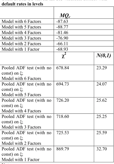
The main focus of this paper is the empirical analysis of sector specific default rates proxies for the Italian economy. Therefore, it is important, first, to investigate the order of integration of this set of variables. We carry two type of unit root test. First, we use the univariate ADF test developed by Dickey and Fuller (1979) for the null of unit root for each of the sector specific default rates. The results from Table 1 suggest that default rates are stationary only after applying a first difference transformation. Then given the low power of the ADF unit root and, given the use, in this paper, of a Dynamic Factor model fitted to a large dataset for the purpose of forecasting and Portfolio Credit Risk modelling, we use the PANIC test recently developed by Bai and Ng (2004) which tests separately for the null of unit root in the factors driving the common component of the full dataset (which includes all the 103 constituents) and in the idiosyncratic component. We apply the PANIC test to the 103 variables dataset where all the series (except the default rates proxies, which are in levels) have been subject to standard transformation (see the appendix for more details regarding the transformation) for the purpose of factor analysis. The PANIC test results can be described as follows. First, from Table 2, according to MQc test statistics for the null of unit root (with only intercept) developed by Bai and Ng (2004), any factor model with the number of principal components varying from six to one (according to the sequential order testing suggested by the authors) is shown to be stationary, given that the null of unit root is always rejected (see the 1% critical values in the footnote of Table 2). Also, the χ2 and the standardised Gaussian version of the pooled test on the idiosyncratic component (obtained by subtracting, from the actual time series, the common component, corresponding to the different number of principal components) show evidence of stationary idiosyncratic component for each variable in the dataset considered. To summarise, contrary to the univariate ADF unit root tests, the PANIC procedure suggest that the level of the sector specific default rates proxies is stationary. Therefore, we include the level of default rates proxies in the dataset from which we extract the principal components to carry forecasting and Portfolio Credit Risk analysis.
DF model specifications corresponding to four, five and six principal components, each with either one or two dynamic factors.
As for in sample forecasting performance, we focus on adjusted R2, obtained from OLS regression of each of the observables in the large dataset (including 103 variables) on the principal components. The mean values of the adjusted R2 for the whole dataset corresponding to four, five and six principal components are 0.50, 0.54, 0.57, respectively. Furthermore, the mean values of the adjusted R2 for the 24 default rates constituents of the whole dataset corresponding to four, five and six principal components are 0.62, 0.66, 0.68, respectively.
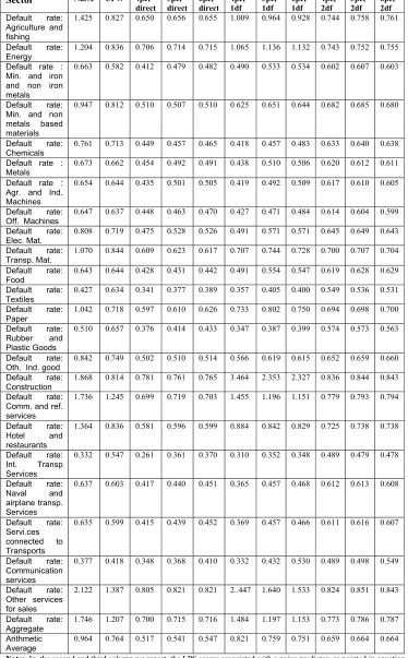
6.3 Empirical Evidence: forecast evaluation
Textiles, Rubber and Plastic Goods, when using the indirect method of forecasting through the use of two dynamic factors; Construction, when using the indirect method of forecasting through the use of one dynamic factors; Int. Transport Services, when we use any type of projection method (except direct prediction through four principal components) or Communication Services, when we use any type of projection method (except direct prediction through four principal components, or the indirect method of forecasting with one dynamic factor and four or five principal components). The direct and indirect method of forecasting through principal components also outperforms a Credit Portfolio View reduced form type of modelling approach (see also Virolainen, 2004) as described in equation (13). Specifically, the associated average QPS and LPS scores are equal to 0.549 and 0.764, respectively.
6.4 Portfolio Credit Risk estimation
7 Conclusions
rates) which might be left ignored when using a few principal components model specification, leading to an underestimation of credit risk.
References
Alves, I. (2004) “Sectoral fragility: factors and dynamics”, BIS Papers no. 22.
Bai, J. and Ng, S. (2004) “A PANIC Attack on Unit Roots and Cointegration”. Econometrica, 72 (4), 1127-1177.
Caling, K., Jacobson T., Lind, J. and K. Roszbach (2006): “Corporate Credit Risk Modeling and the Macroeconomy”. Journal of Banking and Finance, forthcoming.
Cespedes, J.C.G, Herrero, J., Kreinin, A. and D. Rosen (2006) “A Simple Multi-Factor “Factor Adjustment” for the Treatment of Credit Capital Diversification”, Journal of Credit Risk, forthcoming
Dickey, D. A. and Fuller, W. A. (1979), “Distribution of the Estimators for Autoregressive Time Series with a Unit Root”, Journal of the American Statistical Association 74, 427–431.
Elsinger, Helmut, Alfred Lehar, and Martin Summer, 2002, “Risk Assessment for Banking Systems,” Östereichische Nationalbank Working Paper No. 79.
Finger, C. (1999) “Conditional approaches for CreditMetrics portfolio distributions”. CreditMetrics Monitor 1, 14–33.
Forni, M., Giannone D., Lippi, M., Reichlin L. (2005): “Opening the Black Box: structural factor model versus structural VAR models”, Universite Libre de Bruxelles, mimeo
Gordy, M. (2003): “A Risk-Factor Model Foundation for Ratings-Based Bank Capital Rules”,'
Journal of Financial Intermediation, vol. 12 (July 2003), pp. 199-232.
Gupton, G., Finger C., and M. Bhatia. (1997). CreditMetricsTM — Technical Document. J.P. Morgan, New York.
Hamerle, A., Liebig T., and D. Rosch (2003): “Credit Risk Factor Modeling and the Basel II IRB Approach”, Deutsche Bundesbank working paper, no 02/2003.
Hamerle, A. Liebig, T. and Scheule, H. (2004): “Forecasting Credit Portfolio Risk” Deutsche Bundesbank working paper, no 02/2003.
Hanson, S.G., Pesaran H., and Schuermann T. (2005): “Firm heterogeneity and credit risk diversification”, CESifo working paper series no. 1531
Koopman, S.J., Lucas, A. and P. Klaassen (2005): “Empirical Credit Cycles and Capital Buffer Formation”, Journal of Banking and Finance, 29 (12), 3159-3179.
Koopman, S.J., and Lucas, A. (2005): “Business and default cycles for credit risk”, Journal of Applied Econometrics, 20(2), 311-323.
Lucas, A., P. Klaassen, P. Spreij, and S. Straetmans (2001). “An analytic approach to credit risk of large corporate bond and loan portfolios”. Journal of Banking and Finance 25, 1635–1664.
Marcellino, M., Stock, J. H. & Watson, M. W. (2005). A comparison of direct and iterated multistep ar methods for forecasting macroeconomic time series, Journal of Econometrics, forthcoming. Marotta, G., Pederzoli, C., and Torricelli, C.(2005): “Forward looking estimation of default probabilities with Italian data”, Universita’ di Modena e Reggio Emilia, Dipartimento di Economia Politica, working paper no 0504..
Merton, R. (1974). “On the pricing of corporate debt: the risk structure of interest rates”. Journal of Finance 29, 449–470.
Pain, D. (2003) “The Provisioning Experience of the Major UK Banks: A Small Panel investigation.” Bank of England Working Paper No. 177.
Pesaran, H., Schuermann, T., Treutler, B.J. and Weiner, S.W. (2006): “Macroeconomics Dynamics and Credit risk: a global perspective”, Journal of Money, Credit and Banking, 38(5), 1211-1262 Pykhtin, M. (2004) “Multi-factor adjustment”. Risk, 17, 85–90.
Schonbucher, P. (2000): “Factor models for portfolio credit risk” Bonn University working paper Schuermann, T., Pesaran, H.M. and Hanson, S.G. (2005) “Firm Heterogeneity and Credit Risk Diversification”, CESifo working paper no 1531.
Stock and Watson: “Macroeconomic Forecasting using diffusion indices”, Journal of Business and Economic Statistics, 20(2), 147-162
Tasche D. (2005): “ Measuring Diversification in an Asymptotic Multi-Factor Framework”,
Deutsche Bundesbank working paper.
Vasicek O., (2002), “Loan Portfolio Value”, Risk, December, 160-162.
Virolainen, K. (2004): “Macro stress testing with a macroeconomic credit risk model for Finland”,
Bank of Finland working paper, 18-2004.
Wilson, T.C. (1997a): “Portfolio Credit Risk (I)”, Risk, September. (Reprinted in Credit Risk Models and Management. 2004, 2nd edition, edited by David Shimko, Risk Books).
Table 1: ADF unit root test on default rates
Sector ADF
t –statistic on levels
ADF t –statistic on first diff
Default rate: Agriculture and fishing
-1.14 -3.49
Default rate: Energy -1.06 -5.36
Default rate : Minerals and e iron and non iron metals
-2.12 -3.92
Default rate: Default rate: Minerals and non metals based materials
-0.92 -6.22
Default rate:
Chemicals -1.55 -3.82 Default rate : Metals -2.31 -3.08
Default rate : Agriculture and Industry Machines
-1.84 -3.82
Default rate: Office
Machines -1.91 -5.89 Default rate: Electric
Materials -1.37 -4.06 Default rate:
Transport Materials -1.43 -4.98 Default rate: Food -1.83 -3.65 Default rate:
Textiles -2.90 -3.80 Default rate: Paper -1.77 -3.80 Default rate: Rubber
and Plastic Goods -2.11 -4.00 Default rate: Other
industrials good -1.28 -3.63 Default rate:
Construction -0.90 -4.25
Default rate: Commerce and refurbishing
services
-0.89 -3.62
Default rate: Hotel
and restaurants -0.99 -3.00 Default rate: Internal
Transport Services -2.20 -5.44 Default rate: Naval
and airplane transport services -1.64 -3.83 Default rate: Services connected to Transports -1.64 -3.83 Default rate: Communication services -3.18 -4.97
Default rate: Other
services for sales -0.86 -3.96 Default rate:
Aggregate -1.24 -3.64
Note: The lag order for the ADF regression is equal to 4*(T/100)^1/4
Table 2: PANIC test on the 103 variables dataset with default rates in levels
MQc
Model with 6 Factors -87.63 Model with 5 Factors -88.77 Model with 4 Factors -81.46 Model with 3 Factors -76.90 Model with 2 Factors -66.11 Model with 1 Factor -68.93
χ2 N(0,1)
Pooled ADF test (with no const) on ξ;
Model with 6 Factors
678.84 23.29
Pooled ADF test (with no const) on ξ;
Model with 5 Factors
694.73 24.07
Pooled ADF test (with no const) on ξ;
Model with 4 Factors
726.20 25.62
Pooled ADF test (with no const) on ξ;
Model with 3 Factors
718.60 25.25
Pooled ADF test (with no const) on ξ;
Model with 2 Factors
725.53 25.59
Pooled ADF test (with no const) on ξ;
Model with 1 Factor
869.79 32.70
Note: From Table I in Bai and Ng (2004), the 1% critical values for the MQc
Table 3: QPS scores
Sector Naive CPW 4pc; direct 5pc; direct 6pc; direct 4pc; 1df 5pc; 1df 6pc; 1df 4pc; 2df 5pc; 2df 6pc; 2df Default rate: Agriculture and fishing
1.113 0.630 0.458 0.463 0.463 0.799 0.759 0.727 0.551 0.564 0.568
Default rate: Energy
0.962 0.634 0.512 0.520 0.520 0.825 0.900 0.899 0.550 0.558 0.561
Default rate : Min. and iron and non iron metals
0.470 0.390 0.240 0.295 0.298 0.304 0.343 0.344 0.409 0.414 0.411
Default rate: Min. and non metals based materials
0.743 0.616 0.324 0.322 0.324 0.433 0.459 0.452 0.488 0.492 0.487
Default rate: Chemicals
0.567 0.519 0.268 0.275 0.284 0.248 0.285 0.303 0.440 0.447 0.445
Default rate : Metals
0.480 0.469 0.275 0.308 0.307 0.262 0.323 0.319 0.428 0.419 0.418
Default rate : Agr. and Ind. Machines
0.461 0.451 0.259 0.315 0.319 0.247 0.306 0.321 0.424 0.417 0.413
Default rate: Off. Machines
0.454 0.444 0.271 0.282 0.289 0.248 0.288 0.300 0.421 0.411 0.406
Default rate: Elec. Mat.
0.613 0.525 0.292 0.340 0.338 0.307 0.381 0.380 0.452 0.456 0.450
Default rate: Transp. Mat.
0.855 0.646 0.419 0.432 0.426 0.514 0.551 0.535 0.507 0.514 0.511
Default rate: Food
0.450 0.451 0.254 0.257 0.265 0.304 0.362 0.356 0.426 0.435 0.436
Default rate: Textiles
0.249 0.441 0.192 0.215 0.223 0.202 0.234 0.231 0.358 0.345 0.341
Default rate: Paper
0.831 0.525 0.407 0.419 0.435 0.539 0.601 0.555 0.500 0.505 0.507
Default rate: Rubber and Plastic Goods
0.321 0.464 0.211 0.240 0.256 0.192 0.220 0.228 0.382 0.381 0.371
Default rate: Oth. Ind. good
0.645 0.556 0.317 0.325 0.328 0.376 0.427 0.423 0.459 0.466 0.467
Default rate: Construction
1.341 0.619 0.586 0.566 0.568 1.665 1.477 1.459 0.640 0.649 0.648
Default rate: Comm. and ref. services
1.281 0.901 0.506 0.525 0.510 1.123 0.948 0.916 0.585 0.599 0.600
Default rate: Hotel and restaurants
1.073 0.638 0.390 0.405 0.408 0.684 0.646 0.634 0.532 0.545 0.545
Default rate: Int. Transp Services
0.183 0.356 0.149 0.200 0.207 0.175 0.195 0.193 0.302 0.293 0.292
Default rate: Naval and airplane transp. Services
0.444 0.412 0.242 0.262 0.271 0.213 0.278 0.288 0.420 0.420 0.415
Default rate: Servi.ces connected to Transports
0.443 0.408 0.240 0.261 0.272 0.216 0.278 0.286 0.418 0.423 0.415
Default rate: Communication services
0.210 0.247 0.192 0.209 0.236 0.189 0.182 0.325 0.301 0.310 0.357
Default rate: Other services for sales
1.430 0.928 0.609 0.624 0.624 1.493 1.217 1.168 0.629 0.656 0.647
Default rate: Aggregate
1.286 0.899 0.506 0.522 0.522 1.138 0.947 0.916 0.579 0.592 0.593
Arithmetic Average
0.704 0.549 0.338 0.358 0.362 0.529 0.525 0.523 0.467 0.471 0.471
Table 4: LPS scores
Sector Naive CPW 4pc; direct 5pc; direct 6pc; direct 4pc; 1df 5pc; 1df 6pc; 1df 4pc; 2df 5pc; 2df 6pc; 2df Default rate: Agriculture and fishing
1.425 0.827 0.650 0.656 0.655 1.009 0.964 0.928 0.744 0.758 0.761
Default rate: Energy
1.204 0.836 0.706 0.714 0.715 1.065 1.136 1.132 0.743 0.752 0.755
Default rate : Min. and iron and non iron metals
0.663 0.582 0.412 0.479 0.482 0.490 0.533 0.534 0.602 0.607 0.603
Default rate: Min. and non metals based materials
0.947 0.812 0.510 0.507 0.510 0.625 0.651 0.644 0.682 0.685 0.680
Default rate: Chemicals
0.761 0.713 0.449 0.457 0.465 0.418 0.457 0.483 0.633 0.640 0.638
Default rate : Metals
0.673 0.662 0.454 0.492 0.491 0.438 0.510 0.506 0.620 0.612 0.611
Default rate : Agr. and Ind. Machines
0.654 0.644 0.435 0.501 0.505 0.419 0.492 0.509 0.617 0.610 0.605
Default rate: Off. Machines
0.647 0.637 0.448 0.463 0.470 0.427 0.471 0.484 0.614 0.604 0.599
Default rate: Elec. Mat.
0.808 0.719 0.475 0.528 0.526 0.491 0.571 0.571 0.645 0.649 0.643
Default rate: Transp. Mat.
1.070 0.844 0.609 0.623 0.617 0.707 0.744 0.728 0.700 0.707 0.704
Default rate: Food
0.643 0.644 0.428 0.431 0.442 0.491 0.554 0.547 0.619 0.628 0.629
Default rate: Textiles
0.427 0.634 0.341 0.377 0.389 0.357 0.405 0.400 0.549 0.536 0.531
Default rate: Paper
1.042 0.718 0.597 0.610 0.626 0.733 0.802 0.750 0.694 0.698 0.700
Default rate: Rubber and Plastic Goods
0.510 0.657 0.376 0.414 0.433 0.347 0.387 0.399 0.574 0.573 0.563
Default rate: Oth. Ind. good
0.842 0.749 0.502 0.510 0.514 0.566 0.619 0.615 0.652 0.659 0.660
Default rate: Construction
1.868 0.814 0.781 0.761 0.765 3.464 2.353 2.327 0.836 0.844 0.843
Default rate: Comm. and ref. services
1.736 1.245 0.699 0.719 0.703 1.455 1.196 1.151 0.779 0.793 0.794
Default rate: Hotel and restaurants
1.364 0.836 0.581 0.596 0.599 0.884 0.842 0.829 0.725 0.738 0.738
Default rate: Int. Transp Services
0.332 0.547 0.261 0.361 0.370 0.310 0.352 0.348 0.489 0.479 0.478
Default rate: Naval and airplane transp. Services
0.637 0.603 0.417 0.440 0.451 0.365 0.457 0.468 0.612 0.613 0.608
Default rate: Servi.ces connected to Transports
0.635 0.599 0.415 0.439 0.452 0.369 0.457 0.466 0.611 0.616 0.607
Default rate: Communication services
0.377 0.418 0.348 0.368 0.410 0.332 0.432 0.530 0.489 0.498 0.549
Default rate: Other services for sales
2.122 1.387 0.805 0.821 0.821 2..447 1.640 1.533 0.824 0.851 0.843
Default rate: Aggregate
1.746 1.207 0.700 0.715 0.716 1.484 1.197 1.153 0.773 0.786 0.787
Arithmetic Average
0.964 0.764 0.517 0.541 0.547 0.821 0.759 0.751 0.659 0.664 0.664
Table 5: Credit Portfolio Risk corresponding to direct forecasts through DF model
4 static factors
5 static factors
6 static factors Expected
Loss
0.221 0.221 0.221 99.9% VaR 0.443 0.446 0.454 Unexpected
Loss
0.221 0.224 0.232 Expected
Shortfall
[image:25.612.74.326.256.363.2]0.468 0.477 0.484 Note: numbers are in percentages of total exposure
Table 6: Credit Portfolio Risk corresponding to indirect forecasts through DF model: the case of one dynamic factor
4 static factors
5 static factors
6 static factors Expected
Loss
0.221 0.221 0.221 99.9% VaR 0.280 0.365 0.555 Unexpected
Loss
0.058 0.143 0.333 Expected
Shortfall
0.286 0.379 0.603 Note: numbers are in percentages of total exposure
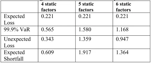
Table 7: Credit Portfolio Risk corresponding to indirect forecasts through DF model: the case of two dynamic factors
4 static factors
5 static factors
6 static factors Expected
Loss
0.221 0.221 0.221 99.9% VaR 0.565 1.580 1.168 Unexpected
Loss
0.343 1.359 0.947 Expected
Shortfall
[image:25.612.73.327.401.506.2]DATA
Code Data description Transformation
EUR001M Euribor 1 mesi 3
EUR003M Euribor 3 mesi 3
EUR006M Euribor 6 mesi 3
ILRSGVTG Italy rendistato govt bond 3
ITISCOKE COKE SA SALES 3
ITISELEC ELECTRICS SA SALES 3
ITISFOOD FOOD SALES 3
ITISFSAT FOREIGN SALES SA 3
ITISLEAT LEATHER SA SALES 3
ITISMACH MACHINERY SA SALES 3
ITISMANF MANUFACTORING SA SALES 3
ITISMETL METALS SA SALES 3
ITISMINE MINERALS SA SALES 3
ITISNMET NON METALS SA SALES 3
ITISNSAT DOMESTIC SALES SA 3
ITISOTHR OTHERS SA SALES 3
ITISPAPR PAPER SA SALES 3
ITISRUBB RUBBER SA SALES 3
ITISSCO CONSUPTION GOODS SA SALES 3
ITISSEN ENERGY SA SALES 3
ITISSIN INVESTIMENT GOODS SA SALES 3
ITISSINT INTERM GOODS SA SALES 3
ITISTEXT TEXTILES SA SALES 3
ITISTRAN TRANSPORT SA SALES 3
ITISTSAT TOTAL SALES SA 3
ITISWOOD WOOD SA SALES 3
ITORFSAL ITALY FOREIGN INDUSTRIAL ORDER SA 3 ITORNSAL ITALY NATIONAL INDUSTRIAL ORDER SA 3
ITORTSAL ITALY INDUSTRIAL ORDER SA 3
ITPIRES ITALY REAL GDP EXPORTS SA WDA 3
ITPIRIS ITALY REAL GDP IMPORTS SA WDA 3
ITPIRLS ITALY REAL GDP SA WDA 3
ITPIRMS ITALY REAL GDP MACHINERY SA WDA 3
ITPIRNS ITALY REAL GDP INVESTIMENTS SA WDA 3 ITPIROS ITALY REAL GDP CONSTRUCTION SA WDA 3 ITPIRPCS ITALY REAL GDP PRIVATE CONSUMPTION SA WDA 3 ITPIRSS ITALY REAL GDP CONSTANT PRICE CHANGE IN STOCKS SA WDA 3 ITPIRTCS ITALY REAL GDP CONSUMPTION SA WDA 3 ITPIRTCW ITALY REAL GDP TRANSPORTS SA WDA 3 ITPIRUCS ITALY REAL GDP PUBLIC CONSUMPTION SA WDA 3 ITPRENS ITALY INDUSTRIAL PRODUCTION ENERGY SA 3 ITPRINS ITALY INDUSTRIAL PRODUCTION INVESTIMENT GOODS SA 3 ITPRITS ITALY INDUSTRIAL PRODUCTION INTERMED GOODS SA 3
ITPRSAN ITALY INDUSTRIAL PRODUCTION SA 3
ITPRSLI ITALY INDUSTRIAL PRODUCTION LEATHER SA 3 ITPRSNI ITALY INDUSTRIAL PRODUCTION NON METALS SA 3 ITPRSOI ITALY INDUSTRIAL PRODUCTION OTHER SA 3 ITPRSPI ITALY INDUSTRIAL PRODUCTION PAPER SA 3 ITPRSRI ITALY INDUSTRIAL PRODUCTION RUBBER SA 3 ITPRSSI ITALY INDUSTRIAL PRODUCTION METALS SA 3 ITPRSTI ITALY INDUSTRIAL PRODUCTION TEXTILES SA 3 ITPRSWI ITALY INDUSTRIAL PRODUCTION WOOD SA 3 ITPRSXI ITALY INDUSTRIAL PRODUCTION FURNITURE SA 3
CPALIT ALL ITEM CPI ITALIA 4
CPCLITI CLOTHING AND FOOTWEAR CPI ITALIA 4
CPCMITI COMMUNICATIONSCPI ITALIA 4
CPEDITI EDUCATION CPI ITALIA 4
CPENITI ENERGY CPI ITALIA 4
CPEXITI CORECPI ITALIA 4
CPFDITI FOOD CPI ITALIA 4
CPFNITI FURNISHING CPI ITALIA 4
CPGGITI GOODS CPI ITALIA 4
CPHLITI HEALTH CPI ITALIA 4
CPHRITI RESTURANT AND HOTELS CPI ITALIA 4
CPMSITI MISCELLANEOUS CPI ITALIA 4
CPRNITI RECREATION CPI ITALIA 4
CPTRITI TRANSPORT CPI ITALIA 4
CPXNITI EXCLUDING ENERGY CPI ITALIA 4
PPENIT PPI ENERGY 4
PPMNIT PPI MANUFACTURING ITALIA 4
PPNGIT PPI NON DOURABLE GOODS ITALIA 4
051 Default rate: Agriculture and fishing 2
052 Default rate: Energy 2
053 Default rate : Minerals and e iron and non iron metals 2 054 Default rate: Minerals and non metals based materials 2
055 Default rate: Chemicals 2
056 Default rate : Metals 2
057 Default rate : Agriculture and Industry Machines 2
058 Default rate: Office Machines 2
059 Default rate: Electric Materials 2
060 Default rate: Transport Materials 2
061 Default rate: Food 2
062 Default rate: Textiles 2
063 Default rate: Paper 2
064 Default rate: Rubber and Plastic Goods 2 065 Default rate: Other industrials good 2
066 Default rate: Construction 2
067 Default rate: Commerce and refurbishing services 2
068 Default rate: Hotel and restaurants 2
069 Default rate: Internal Transport Services 2 070 Default rate: Naval and airplane transport services 2 071 Default rate: Services connected to Transports 2 072 Default rate: Communication services 2 073 Default rate: Other services for sales 2
000 Default rate: Aggregate 2