Modeling a Multivariate Transaction Process
Ingmar Nolte
University of Konstanz, CoFE
abstract
In this paper the dynamics of a joint transaction process are investigated. The transaction process is characterized by four marks: price changes, transaction volumes, bid–ask spreads and intertrade durations. Based on a copula approach, a model for their joint density is proposed, which avoids forcing a priori assumptions on the instantaneous causality relationships between the four variables as necessary in decomposition models, where the joint density is decomposed into its conditional and unconditional densities. The price change process is treated as a discrete process and specified with an integer count hurdle model and the transaction volumes, bid–ask spreads, and trade durations processes are modeled along the lines of fractionally integrated autoregressive conditional models, which are suited very well to capture the high persistency, empirically observed in these processes. The model is applied to three stocks traded at the New York Stock Exchange (NYSE) in May, 2001 and we investigate several market microstructure hypotheses in the empirical part of this paper.
keywords:copula functions, discrete price changes, fractionally integrated autoregressive conditional duration models, integer count hurdle model, market microstructure, transaction data.
I gratefully acknowledge the financial support by the Fritz Thyssen Stiftung through the project “Dealer-Behavior and Price-Dynamics on the Foreign Exchange Market”. I would like to thank Eric Renault (editor), the co-editor and two anonymous referees for constructive suggestions on previous drafts of the paper. Special thanks go to Nikolaus Hautsch, Sandra Nolte, Winfried Pohlmeier, and Valeri Voev, the participants of the conference “The Econometrics of the Microstructure of Financial Markets,” April 23–24, 2004, CentER, Tilburg University, and the participants of the “59th European Meeting of the Econometric Society” August 20–24, 2004, Madrid for helpful comments. Address for correspondence: Department of Economics, Box D124, University of Konstanz, 78457 Konstanz, Germany. Tel.: +49-7531-88-3753; Fax: +4450, email: [email protected].
doi: 10.1093/jjfinec/nbm020
Advance Access publication November 22, 2007
C
The Author 2007. Published by Oxford University Press. All rights reserved. For permissions,
please e-mail: [email protected].
at Lancaster University on July 11, 2013
http://jfec.oxfordjournals.org/
1 Introduction
The empirical analysis of market microstructure (MMS) variables allows us to infer how market participants process information, submit orders with a specific volume at a specific time, interact with each other, and affect the price process of an asset. The results from these analyses are of utmost importance for the efficient design of the institutional setup and the trading systems in financial markets. Moreover, they are on one hand the basis for the development of theoretical MMS models and on the other they allow us to verify existing models empirically.
The importance being attributed to empirical MMS research is underpinned by an enormous amount of very well written papers in this field of research in the last two decades. Engle (1982), Bollerslev (1986), Hausman, Lo, and MacKinlay (1992), Hasbrouck and Sofianos (1993), O’Hara (1995), Engle and Russell (1998), Engle (2000), Dufour and Engle (2000), Ghysels, Gourieroux, and Jasiak (2004) represent only a tiny part thereof.
However, most of the existing studies do not analyze relationships between several MMS variables based on a joint model for these variables. Instead, the relationship between a set of MMS variables, such as price changes, volatility, transaction volumes, bid–ask spreads and intertrade durations is analyzed in uni-variate models; see Hausman, Lo, and MacKinlay (1992) and Dufour and Engle (2000) for example, or in decomposition models, see Russell and Engle (2002), Ryd-berg and Shephard (2003) and Manganelli (2005). In these models, one of the MMS variables is treated as the left-hand variable and the rest as covariates assuming an a priori instantaneous causality relationship between these variables or imposing a strict exogeneity assumption in the sense of Engle, Hendry, and Richard (1983). An exception is the study by Renault and Werker (2006), where the instantaneous causality effect between volatility and trade arrival times is disentangled from the Granger causality effects between these variables.
In this paper, we pick up the suggestion of Dufour and Engle (2000) and for-malize a model for the joint system of price changes, transaction volumes, bid–ask spreads and intertrade durations, which, from our point of view, are four of the most important MMS variables. We rely on a copula approach to separate instanta-neous causality effects from Granger causality effects and we avoid decomposing the joint process into conditional and marginal processes and postulating a par-ticular instantaneous causality scheme between the four MMS variables a priori. Moreover, in the specification of the marginal processes, we try to take the most important MMS characteristics such as discreteness of price changes as well as the high persistency of transaction volumes, bid–ask spreads and intertrade durations into account. We use the Liesenfeld, Nolte, and Pohlmeier (2006) dynamic integer count hurdle (ICH) model for the specification of the discrete price change process, whereas the processes for transaction volumes, bid–ask spreads, and intertrade durations are modeled with fractionally integrated autoregressive conditional du-ration (FIACD) type models proposed by Jasiak (1999). The application of ACD-type models to transaction volumes and bid–ask spreads is unproblematic since by definition both variables have a positive outcome space. For transaction volumes,
at Lancaster University on July 11, 2013
http://jfec.oxfordjournals.org/
ACD-type models have already been proposed by Manganelli (2005). Since, we are considering a four-dimensional process in which one component is discrete (price changes) and the remaining three components are continuous, we rely for the price change variable on the continuation approach suggested by Stevens (1950), Heinen and Rengifo (2007) and Denuit and Lambert (2005) during the specification of the copula function.
The empirical analysis is carried out, using data from the NYSE Trade and Quote (TAQ2) database, for three stocks: Black & Decker Corporation (BDK), In-ternational Business Machines (IBM), and Coca-Cola Company (KO), traded at the NYSE for the period from May 1, 2001 to May 31, 2001. We can show that the proposed model specification fits the dynamics of the joint process very well and we apply our model to verify several market microstructure hypotheses. We find, that the role of trade arrival times in explaining bid–ask spreads (Foster and Viswanathan (1990)) and price change volatility (Easley and O‘Hara (1992), Dufour and Engle (2000)) is diminished and ambiguous, when controlling for the informa-tion conveyed by the transacinforma-tion volume and the bid–ask spread processes.
The rest of the paper is structured in the following way: Section 2 presents the model in detail, Section 3 contains the empirical analysis as well as the application to market microstructure hypotheses, and Section 4 concludes the paper.
2 Multivariate Modeling
LetPt∈ς·Zdenote the transaction price at thetth trade, whereς∈R+denotes
the tick size andt=(0), 1, . . . ,T. The associated (standardized) price change from the (t−1)th to thetth trade is then given byCt≡(Pt−Pt−1)/ς∈Z, the volume
traded at thetth trade is denoted byVt ∈R+, the bid–ask spread at thetth trade
is denoted bySt∈R+, and the duration between the (t−1)th and thetth trade is
denoted byDt ∈R+.
We collect these marks of the transaction process in the vectorMt∈Z×R+3:
Mt≡(Ct,Vt,St,Dt),
we setFt ≡σ(Ms|s≤t) and denoteθas the generic overall parameter vector. Our
aim is to model the conditional joint density of Mt denoted by fMt(mt|Ft−1;θ) within a parametric framework. We want to avoid a specification, where the joint density is decomposed into a product of sequential conditional densities and a marginal density, since such a specification imposes a specific form on the instan-taneous causality relationship of the variables under consideration. Therefore we decide to rely on a copula approach, which allows for a direct investigation of the instantaneous relationships in our system, rather than simply choosing that spec-ification which seems to be the most reasonable according to our current market microstructure knowledge. Choosing the copula approach, we are, in particular, able to manage and investigate different instantaneous relationship patterns sepa-rately from their Granger causality effects between our variables across stocks.
at Lancaster University on July 11, 2013
http://jfec.oxfordjournals.org/
The joint distribution function ofMt denoted by1 FMt(mt|Ft−1) can be related to its marginal distributions using the copula functionC: [0, 1]4→[0, 1] as
FMt(mt|Ft−1)=C
FCt(ct|Ft−1),FVt(vt|Ft−1),FSt(st|Ft−1),FDt(dt|Ft−1)
,
whereFCt,FVt,FSt andFDtdenote the marginal distribution functions of the price change, the volume, the bid–ask spread and the duration, respectively. Sklar (1959) proved the existence of the copula functionCand showed its uniqueness on [0, 1]k
for the case where allkvariables of the joint distribution function are continuous. In that case, one can take the derivative of the joint distribution function with respect to its components to obtain a valid specification for the joint density.
Also, according to Sklar (1959) in the case where certain components of the joint density are discrete, asCt in our case, we do not achieve uniqueness of the
copula function, in our case on [0, 1]4, but only on Range(F
Ct)×[0, 1]
3. The joint
density function can then be obtained either by approximating the derivative of
FMt(mt|Ft−1) with respect toCt by a finite difference as proposed by Meester and MacKay (1994) and Cameron, Li, Trivedi, and Zimmer (2004) or by artificially con-tinuingCtand computing the usual derivative based on the continuedCtas
sugges-ted by Stevens (1950), Heinen and Rengifo (2007) and Denuit and Lambert (2005). In this paper, we rely on the latter strategy and we continue the discrete variable
Ct, following Denuit and Lambert (2005) with the help ofUt being independent
uniformlyU(0, 1) distributed, by setting
Ct∗≡Ct−Ut,
where Ct∗∈R denotes the continued price change variable. With Mt∗ be-ing the vector Mt, where Ct has been replaced by Ct∗, and FCt∗ being the distribution function of C∗t, we can obtain the joint density fMt∗(m
∗
t|Ft−1)=
(∂4F
Mt∗(m
∗
t|Ft−1))/∂Ct∗,∂Vt,∂St,∂Dtas
fMt∗(m
∗
t|Ft−1)= fC∗t(c
∗
t|Ft−1)· fVt(vt|Ft−1)· fSt(st|Ft−1)· fDt(dt|Ft−1)
cFCt∗(c
∗
t|Ft−1),FVt(vt|Ft−1),FSt(st|Ft−1),FDt(dt|Ft−1)
, (1)
wherecdenotes the density of the copula functionC. Since, we will specify a model forCt, we need the relationship between the discrete distribution function ofCt
and the continuous distribution function ofCt∗for the computation of the copula density. SinceC∗t ≤Cta.s. and the integer partCt∗ of the continuous variableCt∗
is given byCt∗ =Ct−1 we obtainFCt∗(c
∗
t) as
FCt∗(c
∗
t)=P(Ct∗≤c∗t)=P(C∗t ≤ c∗t )+P(c∗t <Ct∗≤c∗t) =P(C∗t ≤ct−1)+P(ct−1<C∗t ≤ct∗)
=P(Ct≤ct−1)+P(ct−1<Ct−Ut≤ct−ut) =P(Ct≤ct−1)+P(Ut ≤ut)·P(Ct=ct) = FCt(ct−1)+ut· fCt(ct),
1For the ease of notation we suppress the parameter vectorθ.
at Lancaster University on July 11, 2013
http://jfec.oxfordjournals.org/
where the last equation follows from the fact that forUt∼U(0, 1), P(Ut≤ut)=ut.
Moreover, we used the relationship that P(Ct∗≤ct−1)=P(Ct ≤ct−1) sincectis
discrete. Please note, that the specification in Equation (1) is based on a fixed or unconditional copulaCin that sense, that the copula function itself is not assumed to be time-varying or dependent onFt. Such an extension, which has been proposed by Patton (2001 and 2006), would increase the computational burden in our model considerably.
2.1 Specification of the Marginal Densities and the Copula Function
We now address the specification of the marginal densities of the price change, the volume, the bid–ask spread, and the duration processes as well as the choice of the copula function.
2.1.1 Price change process We apply the ICH model of Liesenfeld, Nolte, and
Pohlmeier (2006), to model the discrete density of the price change
fCt(ct|Ft−1).
The idea of the ICH model is to decompose the price change process into two components: (i) a direction process and (ii) a size or an absolute price change process given a nonzero price change.
Letπjt, j ∈ {−1, 0, 1}denote the conditional probability of a negative P(Ct <
0|Ft−1), a zero P(Ct =0|Ft−1) or a positive price change P(Ct>0|Ft−1) at timet. The
conditional density of a price change is then specified as
fCt(ct|Ft−1)=π−1t
1l{Ct<0}·π
0t1l{Ct=0}·π1t1l{Ct>0}· f|Ct|(|ct| |Ct=0,Ft−1)
1−1l{Ct=0}
,
where f|Ct|(|ct| |Ct =0,Ft−1) denotes the conditional density of an absolute price change, with supportN\ {0}.
To obtain a parsimoniously specified model, we adopt the simplification of Liesenfeld, Nolte, and Pohlmeier (2006), that the conditional density of an absolute price change stems from the same distribution irrespective of whether it is an upward or a downward price change.
2.1.1.1 Direction process In order to model the conditional probabilities of the direction process, we use the autoregressive conditional multinomial (ACM) model of Russell and Engle (2002) with a logistic link function, given by
πjt=
exp(jt)
1
j=−1exp(jt)
(2)
with normalizing constraint0t =0, ∀t. The resulting vector of log-odds ratios t≡(−1t,1t)=(ln[π−1t/π0t], ln[π1t/π0t])is specified as a multivariate
ARMA-type model:
(I2−βp(L))(t−ζr(L) ln(Zt))=µ+αq(L)εt+γs(L)|εt|, (3)
at Lancaster University on July 11, 2013
http://jfec.oxfordjournals.org/
whereαq(L),βp(L), andγs(L) denote 2×2 matrix valued lag polynomials of
or-der q,p, ands, respectively. Zt =(Vt,St,Dt) denotes the vector of explanatory
variables—volume, bid–ask spread, and duration—which are included statically and in lagged form through the 2×3 matrix valued lag polynomialζr(L) of order
rin this specification.µdenotes the 2×1 vector of constants, and the innovation vector of the ARMA model is specified as martingale differences given by
εt ≡(ε−1t,ε1t), where εjt≡
xjt−πjt
πjt(1−πjt)
, j∈ {−1, 1}, (4)
and
xt≡(x−1t,x1t)=
⎧ ⎨ ⎩
(1, 0) if Ct<0
(0, 0) if Ct=0
(0, 1)if Ct >0,
(5)
denotes the 2×1 state vector indicating the direction of the price movement at timet. Thus,εtrepresents the standardized state vectorxt. Note, that we included
also the absolute innovation term|εt|to capture asymmetries in the news impact
curve for the log odds ratios.
2.1.1.2 Absolute price change process The conditional density of the absolute price process is modeled with an at-zero-truncated Negative Binomial (NegBin) distribution, given by
f|Ct|(|ct| |Ct=0,Ft−1)≡
(κ+ |ct|) (κ)(|ct| +1)
κ+ωt κ
κ
−1
−1 ω
t ωt+κ
|ct| , (6)
where|ct| ∈N\ {0},κ >0 denotes the dispersion parameter andωt is
parameter-ized using the logarithmic link function with a generalparameter-ized autoregressive moving average specification (GLARMA) of Shephard (1995) in the following way:
(1−β˜p(L))(lnωt−δ˜D˜t−ζ˜r(L) ln(Zt))=µ˜+S(ν,τ,K)+α˜q(L)˜εt+γ˜s(L)|ε˜t|, (7)
where ˜Dt∈ {−1, 1}indicates a negative or a positive price change at timetwith
cor-responding coefficient ˜δ.Zt=( ˜Dt,Vt,St,Dt)denotes again the vector of further
explanatory variables, with associated 1×4 dimensional parameter lag polyno-mialζr(L). ˜αq(L), ˜βp(L), and ˜γs(L) denote scalar lag polynomials, ˜µthe constant
and
S(ν,τ,K)≡ν0τ+
K
k=1
ν2k−1sin(2π(2k−1)τ)+ν2kcos(2π(2k)τ) (8)
a Fourier flexible form to capture intraday seasonality in the absolute prices changes, which can be considered as a measure for volatility, whereτ is the intra-day trading time standardized to [0, 1] andνis a 2K +1 dimensional parameter vector. In the spirit of Nelson (1991) for GARCH and Dufour and Engle (2000) for ACD models, we include again an absolute innovation term|ε˜t|to allow for an
at Lancaster University on July 11, 2013
http://jfec.oxfordjournals.org/
asymmetric news response of lnωt. ˜εtconstructed as
˜
εt≡ |
Ct| −E(|Ct| |Ct=0,Ft−1)
Var(|Ct| |Ct=0,Ft−1)1/2 ,
is the innovation term that drives the GLARMA model. For a more elaborate presentation of the ICH model and its components as well as for some stationarity considerations we refer the reader to Liesenfeld, Nolte, and Pohlmeier (2006).
2.1.2 Transaction volume, bid–ask spread and trade duration processes
Since we consider transaction volume, bid–ask spread, and trade duration as variables with a positive real domain, we specify their conditional densities in a similar way and we decide to present their models in a unified notation with
Yt∈ {Vt,St,Dt}. Thus, we are concerned with the conditional density
fYt(Yt|Ft−1),
and we specify fYt(Yt|Ft−1) within the autoregressive conditional duration (ACD) framework introduced by Engle and Russell (1998). Manganelli (2005) already showed that the transaction volume process can be reasonably modeled using ACD specifications and we apply this approach to the bid–ask spread process as well. There are several extensions to the original ACD model, see for example Bauwens, Giot, Grammig, and Veredas (2004), Lunde (2000), Grammig and Maurer (2000), and Bauwens and Hautsch (2006). Here, we rely on the FIACD model of Jasiak (1999), which we augment by a multiplicative function to capture intraday seasonality.
Thus, we assume that the variableYtconsists multiplicatively of a seasonality
functions(ν,τ,K), a conditional mean functionϕt(θY|Ft−1), and an error termεt:
Yt=s(ν,τ,K)·ϕt(θY|Ft−1)·εt, εt∼i.i.d. ˜fYt(·),
where ˜fYt(·) is an error term density with unit mean. Assuming ˜fYt(·) to be in-dependent of the conditioning informationFt−1facilitates modeling, since we do
not need to be concerned with higher conditional moments. An extension that allows for separate dynamics in the conditional variance is presented by Ghysels, Gourieroux, and Jasiak (2004). Applying the transformation theorem2yields
Yt∼
1
sϕt
˜
fYt
yt
sϕt
, (9)
wheres≡s(ν,τ,K) andϕt ≡ϕt(θY|Ft−1). To ensure a positive seasonality function
we assumes(ν,τ,K)=exp(S(ν,τ,K)) whereS(ν,τ,K) follows a Fourier flexible form as stated in Equation (8). We specify ˜fYt(·) as an exponential density with unit mean, i.e., ˜fYt(·)∼Exp(1) and the dynamics of the conditional mean function are
2See, e.g., Rohatgi (1976), p. 135, Theorem 6.
at Lancaster University on July 11, 2013
http://jfec.oxfordjournals.org/
modeled according to Jasiak (1999) as
(1−βp(L))ϕt=µ+γ∞(L)Yt, (10)
with a constantµand an infinite-dimensional scalar lag polynomialγ∞(L), given
by
γ∞(L)=[1−βp(L)−[1−αq(L)−βp(L)](1−L)d],
whereαq(L) andβp(L) denote scalar lag polynomials and (1−L)d, 0<d<1 the
fractional differencing operator given by
(1−L)d =
∞
k=0 kLk,
with
k=
(k−d)
(k+1)(−d)=
0<j≤k
j−1−d
j , k=0, 1, 2, . . .
and(·) the gamma function defined as
(x)≡ ⎧ ⎪ ⎪ ⎨ ⎪ ⎪ ⎩
∞
0
tx−1exp(−t)dtifx>0,
∞ ifx=0,
x−1(1+x) ifx<0.
All coefficients inβp(L) andαq(L) as well asµhave to be nonnegative to ensure
positivity of the conditional mean function (out-of-sample). Jasiak (1999) shows that the FIACD(p,d,q) model is strictly stationary and ergodic for 0≤d≤1, but not weakly stationary, since the first unconditional moment ofYt is infinite, due
to the fact that the fractional differencing operator evaluated at lag L=1 is 0. The FIACD(p,d,q) class nests the classes of ACD(p,q) models ford=0 and their integrated counterparts ford=1.
An important point in the estimation is, that we have only a finite sample of data and therefore the “∞” in (1−L)d=∞
k=0kLk needs to be approximated
and the preceding data points for the initialization need to be set. We set “∞ = 1000” and initiated the foregoing 1000 lags ofYt with the unconditional mean of
Yt. Applying this approximation, we can consider the FIACD(p,d,q) models as
ACD(p,1000+max(p,q)) models, with parameter restrictions of a specific functional form depending ond.
2.1.3 Copula function Let us recall Equation (1), which states the joint
condi-tional density of the trading marks vectorMt∗:
fM∗t(m
∗
t|Ft−1)= fCt∗(c
∗
t|Ft−1)· fVt(vt|Ft−1)· fSt(st|Ft−1)· fDt(dt|Ft−1)
cFC∗t(c
∗
t|Ft−1),FVt(vt|Ft−1),FSt(st|Ft−1),FDt(dt|Ft−1)
.
at Lancaster University on July 11, 2013
http://jfec.oxfordjournals.org/
In this equation, the copula densitycis specified as a four-dimensional Gaussian copula density, given by:
c(y1t,y2t,y3t,y4t;)=det()−0.5exp
1 2q
t(I4−−1)qt
, (11)
where=(ρi j) denotes the 4×4 correlation matrix ofq=(q1t,q2t,q3t,q4t)with
qit=−1(yit),i=1, . . . , 4. Thus, for example, the argumenty1tof the copula
func-tioncis the probability mass in the left tail of the conditional price change distribu-tionFCt∗(·|Ft−1) up to the observed (continued) price changec
∗
t at timet; andq1tis
the quantile of the standard normal distribution associated with that left tail proba-bility. In that senseq1trepresents a kind of “normalized” price change observation
c∗t where the ordering of the observations is not interchanged since FC∗t(·|Ft−1) as well as(·) are strictly monotonically increasing. The observationsvt,st, anddtare
“normalized” toq2t,q3t, andq4t analogously and the correlation matrix
repre-sents the correlation between these “normalized” variables. We redefinein the following way:
=(ρi j)=
⎛ ⎜ ⎜ ⎝
1 ρC V ρC SρC D ρC V 1 ρVSρV D ρC S ρVS 1 ρSD ρC DρV DρSD 1
⎞ ⎟ ⎟
⎠, i,j=C,V,S,D, (12)
to facilitate an intuitive interpretation of the parameters inwith respect to the relations between price changes (C), transaction volumes (V), bid–ask spreads (S), and intertrade durations (D).
3 Empirical Analysis
3.1 Database
In the empirical analysis we use tick-by-tick data from May 1, 2001 to May 31, 2001 of three stocks traded at the NYSE: BDK, IBM, and KO. The data stems from the Trade and Quote (TAQ2) database, which is separated into two files: the trade database and the quote database.
The trade database contains all transaction prices and volumes and the quote database consists of all bid and ask quotes and depths, timestamped to the second. To determine, which bid and ask quotes (bid–ask spread) were valid at a certain trade observation and whether this trade was a buy or a sell, one has to merge the two databases. The common algorithm that has been applied predominantly in the literature is the Lee and Ready (1991) procedure, which relies on a so-called “five-seconds rule,” which means that each trade is assigned to the quotes posted at least 5 seconds before. The identification of a buy or sell is done in the following way: If the transaction price is above (below) the midquote, the trade is defined as a buy (sell); for transaction prices at the midquote, the tick rule applies, i.e., if the
at Lancaster University on July 11, 2013
http://jfec.oxfordjournals.org/
transaction takes place at a higher (lower) price than the price of the most recent trade with a different price, the trade is characterized as a buy (sell).
In the last few years this algorithm has been criticized, e.g., by Boehmer, Grammig, and Theissen (2007) and Vergote (2005) concerning the time span of 5 seconds, which does not seem to be appropriate anymore, due to advances in computer technology. Therefore, we check for which lag value in seconds (between 0 and 5) the number of the transaction prices corresponding exactly to previous quotes is maximized and it turns out that for all three stocks, this occurs at 1 second. Thus, we apply the Lee and Ready (1991) algorithm in a modified way using a delay of 1, instead of 5 seconds only.
A further problem arises due to the fact that in some cases there are several trades at exactly the same timestamp. This can happen due to an automatic match-ing of different orders on one side of the specialist’s book against a larger order on the other side (split-transaction). Moreover, such transactions can also result from different market participants, who posted their orders (electronically) within 1 second or, as pointed out by Veredas, Rodriguez-Poo, and Espasa (2002), by limit orders of different market participants with exactly the same limit, e.g., at round prices. Unfortunately, these differences cannot be identified with the TAQ2 database. We have treated all trades as split transactions, which were recorded at the same second. In this case, we have simply aggregated their volume to one transaction and assigned the last price in the sequence to the aggregated transac-tion. Furthermore, we have removed all trades outside the regular trading hours as well as each day’s first trade, to circumvent contamination due to the opening call auction at the NYSE.
3.2 Descriptive Statistics
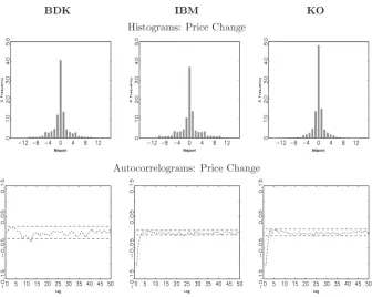
In Figure 1 we have plotted the histograms and the autocorrelograms up to lag 50 for the tick-by-tick price changes of BDK, KO, and IBM. With a mean duration of 53.1, 14.8, and 6.9 seconds, respectively, a lag of 50 corresponds approximately to 44, 12, and 6 minutes.
The histograms show a fairly large support; most of the mass is concentrated between−7 and 7 ticks, but for BDK and IBM even the classes±8,±9, and±10 still possess a mass of around 1% each. The 0 tick classes have frequencies between 40% and 50% and±1 tick classes take frequencies between 10% and 15%. The large support in combination with the high concentration at the 0 tick class, justifies the application of the discrete ICH model. An alternative approach to model the discrete price change process would be the decomposition model of Rydberg and Shephard (2003), which is also capable of modeling discrete outcomes with a fairly large support. The ordered probit model of Hausman, Lo, and MacKinlay (1992) or the multinomial model of Russell and Engle (2002), however, suffer from the drawback that they can only model reliably discrete outcomes with a bounded support. The autocorrelograms of IBM and KO exhibit the usual negative first-order autocorrelation coefficient, which can be explained by the bid–ask bounce
at Lancaster University on July 11, 2013
http://jfec.oxfordjournals.org/
Figure 1 Histograms (first row) and autocorrelograms (second row) of BDK, IBM, and KO price changes. Confidence bands: asymptotic 95%.
effect examined by Roll (1984). For BDK, however, such an effect cannot be observed and all autocorrelation coefficients are basically insignificant.
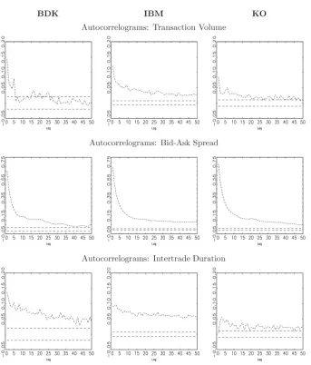
Figure 2 depicts the autocorrelograms, again up to lag 50, of transaction vol-umes, bid–ask spreads, and intertrade durations for all three stocks. Except the transaction volume of BDK, all autocorrelation functions have in common that even the autocorrelation coefficient at lag 50 is still significantly different from zero. The decay of the empirical autocorrelation functions for transaction volumes and intertrade durations is very slow, whereas for the bid–ask spread it is quite fast until, say, lag 10, but from thereon again very slow. Because of these observations, we do not consider the decay of these empirical autocorrelation functions to be exponential and therefore we rely on the fractionally integrated specification for the dynamics of the mean function of transaction volume, bid–ask spread, and duration.
3.3 Estimation Results
All estimation results are obtained by jointly maximizing the log-likelihood im-plied by Equation (1). After a careful model selection procedure, we decide to model the conditional mean functions for all four variables of all three stocks
at Lancaster University on July 11, 2013
http://jfec.oxfordjournals.org/
Figure 2 Autocorrelograms of BDK, IBM, and KO transaction volumes (first row), bid–ask spreads (second row), and intertrade durations (third row). Confidence bands: asymptotic 95%.
with specifications that possess a lag length of 1 for the autoregressive and the innovation variables. We allow the explanatory variables to be lagged up to lag 3. In detail, we specify the conditional mean function in the ACM model for the price change direction (see Equation (3)) as:
(I2−β1(L))(t−ζ3(L) ln(Zt))=µ+α1(L)εt+γ1(L)|εt|, (13)
whereµ,α1,β1,γ1, andζifori=1, 2, 3 are assumed to be symmetric. We impose
these symmetry constraints on the parameters to ensure a parsimonious model
at Lancaster University on July 11, 2013
http://jfec.oxfordjournals.org/
specification.Zt=(Vt,St,Dt)denotes the vector of explanatory variables. To
clar-ify the notation and to ease the interpretation ofζiwith respect to the explanatory
variables, we denote the components ofζiin the following way:
ζi=
ζV i1 ζiS1ζiD1 ζV
i2 ζiS2ζiD2
. (14)
The conditional mean function in the GLARMA model, see Equation (7), for the size of the price change is specified as:
(1−β˜1(L))(lnωt−δ˜D˜t−ζ˜3(L) ln(Zt))=µ˜ +S(ν,τ,K)+α˜1(L)˜εt+γ˜1(L)|ε˜t|, (15)
where ˜Dt∈ {−1, 1}indicates the direction of the contemporaneous price change
at timet, andZt=( ˜Dt,Vt,St,Dt)denotes again the vector of further explanatory
variables. The components of the parameter vectorζi are now denoted as ˜ζi =
( ˜ζD˜
i , ˜ζiV, ˜ζiS, ˜ζiD) andK is set to 2 in the specification of the Fourier flexible form.
In the fractionally integrated models, the conditional mean function (see Equa-tion (10)) is specified as
(1−β1(L))(ϕt−ζ3(L) ln(Zt))=µ+γ∞(L)Yt, (16)
with
γ∞(L)=[1−β1(L)−[1−α1(L)−β1(L)](1−L)d],
where i) for transaction volume, i.e. Yt=Vt, the vector of further explanatory
variables is specified as Zt =(Ct,St,Dt)with parameter vectorζi =(ζiC,ζiS,ζiD),
ii) for the bid–ask spread, i.e.,Yt=St, the vector of further explanatory variables
is specified as Zt=(Vt,Ct,Dt) with parameter vectorζi=(ζiV,ζiC,ζiD), and iii)
for intertrade duration, i.e.,Yt =Dt, the vector of further explanatory variables is
specified asZt=(Vt,St,Ct)with parameter vectorζi=(ζiV,ζiS,ζiC). The parameter
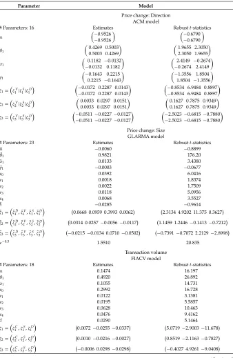
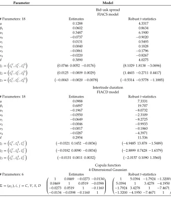
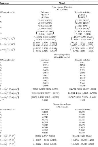
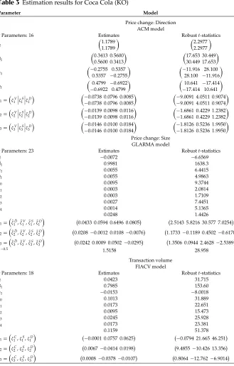
Kin the exponential Fourier flexible forms(ν,τ,K) in Equation (9) is set to 2, again. In Tables 1–3 we report the estimation results of our model for BDK, IBM, and KO, respectively. Before interpreting the results in Section 3.4 in the light of market microstructure applications, we first consider the general pattern of the parameter estimates and the goodness of fit of our models across stocks.
For all three stocks, we find a clear diurnal seasonality pattern (represented by the joint significance ofν) in the duration, the spread, the volume, and the price changes size processes. Since, these patterns coincide with the usual U- and J-shape patterns, see, e.g., Bauwens and Giot (2001), for financial tick-by-tick variables, we do not present their graphs here.
The ACM models responsible for the price change direction process are char-acterized by a moderate degree of persistence: the parameter estimates for the components ofβ1 lie between 0.3 and 0.6; and, they reflect the bid–ask bounce
effect observed for IBM and KO (Figure 1) as well as the absence of it for BDK, through the parameter matricesα1 andγ1, which represent the effect of a
at Lancaster University on July 11, 2013
http://jfec.oxfordjournals.org/
Table 1 Estimation results for Black & Decker (BDK)
Parameter Model
Price change: Direction ACM model
# Parameters: 16 Estimates Robustt-statistics
µ −0.9526 −0.9526 −0.6790 −0.6790 β1 0.4269 0.5003 0.5003 0.4269 1.9655 2.3050 2.3050 1.9655 α1
0.1182 −0.0132 −0.0132 0.1182
2.4149 −0.2674 −0.2674 2.4149
γ1
−0.1643 0.2215 0.2215 −0.1643
−1.3556 1.8504 1.8504 −1.3556
ζ1=ζV 1|ζ1S|ζ1D
−0.0172 0.2287 0.0143
−0.0172 0.2287 0.0143
−0.8534 6.9484 0.8897 −0.8534 6.9484 0.8897
ζ2=ζV 2|ζ2S|ζ2D
0.0033 0.0297 0.0151
0.0033 0.0297 0.0151
0.1627 0.7875 0.9349 0.1627 0.7875 0.9349
ζ3=ζV 3|ζ3S|ζ3D
−0.0511−0.0227−0.0127
−0.0511−0.0227−0.0127
−2.5023−0.6815−0.7880 −2.5023−0.6815−0.7880
Price change: Size GLARMA model
# Parameters: 23 Estimates Robustt-statistics ˜
µ −0.0060 −0.8899
˜
β1 0.9821 176.20
˜
α1 0.0133 3.4380
˜
γ1 −0.0003 −0.0677
ν0 0.0392 6.0416
ν1 0.0018 1.8374
ν2 0.0022 1.7509
ν3 0.0118 5.0956
ν4 0.0068 3.5527
˜
δ −0.0285 −0.9614
˜
ζ1=ζ˜D˜
1, ˜ζ1V, ˜ζ1S, ˜ζ1D
0.0668 0.0959 0.3993 0.0062 2.3134 4.9202 11.375 0.3627 ˜
ζ2=ζ˜D˜
2, ˜ζ2V, ˜ζ2S, ˜ζ2D
0.0314 0.0257−0.0056−0.0117 1.1459 1.2446−0.1413−0.7212 ˜
ζ3=ζ˜D˜
3, ˜ζ3V, ˜ζ3S, ˜ζ3D
−0.0215−0.0134 0.0710−0.0502 −0.7391−0.7072 2.2129−2.8998
κ−0.5 1.5510 20.835
Transaction volume FIACV model
# Parameters: 18 Estimates Robustt-statistics
µ 0.1474 16.197
β1 0.4920 26.892
α1 0.1055 14.731
ν0 0.2992 16.728
ν1 0.0122 3.1381
ν2 0.0195 5.5857
ν3 0.0628 10.463
ν4 0.0476 9.4162
d 0.0290 5.1464
ζ1=ζC 1,ζ1S,ζ1D
0.0072−0.0255−0.0337 5.0719−2.9003−11.678
ζ2=ζC 2,ζ2S,ζ2D
0.0010−0.0216−0.0027 0.8519−2.1163−0.7827
ζ3=ζC 3,ζ3S,ζ3D
−0.0006 0.0298−0.0298 −0.4027 4.9261−9.0408 (Continued)
at Lancaster University on July 11, 2013
http://jfec.oxfordjournals.org/
Table 1(Continued)
Parameter Model
Bid–ask spread FIACS model
# Parameters: 18 Estimates Robustt-statistics
µ 0.1288 4.3317
β1 0.0602 0.8634
α1 0.3487 6.1900
ν0 −0.0737 −0.9020
ν1 0.0131 0.5493
ν2 0.0040 0.1828
ν3 −0.0061 −0.1796
ν4 −0.0220 −0.8267
d 0.3090 4.0275
ζ1=ζV 1,ζ1C,ζ1D
0.0746 0.0052−0.0176 8.1029 1.8138−3.0696
ζ2=ζV 2,ζ2C,ζ2D
0.0125−0.0009 0.0029 1.4603−0.2711 0.4417
ζ3=ζV 3,ζ3C,ζ3D
−0.0043−0.0020−0.0078 −0.5314−0.5778−1.1885 Intertrade duration
FIACD model
# Parameters: 18 Estimates Robustt-statistics
µ 0.0988 7.3331
β1 0.6097 19.707
α1 −0.1967 −8.0732
ν0 −0.0550 −2.3109
ν1 −0.0649 −8.2725
ν2 −0.0046 −0.9933
ν3 −0.0017 −0.1860
ν4 −0.0287 −4.3971
d 0.2954 11.536
ζ1=ζV 1,ζ1S,ζ1C
−0.0321 0.1452−0.0036 −4.9485 13.878−1.5489
ζ2=ζV 2,ζ2S,ζ2C
−0.0182 0.0090−0.0034 −2.8899 0.7428−1.6379
ζ3=ζV 3,ζ3S,ζ3C
−0.0131 0.0011 0.0032 −2.0157 0.1090 1.3560 Copula function
4-Dimensional Gaussian
# Parameters: 6 Estimates Robustt-statistics
=(ρi j),i,j=C,V,S,D
⎛ ⎜ ⎜ ⎝
1 0.0469 −0.0273−0.0134 0.0469 1 0.0519 −0.0398 −0.0273 0.0519 1 −0.1160 −0.0134−0.0398−0.1160 1
⎞ ⎟ ⎟ ⎠ ⎛ ⎜ ⎜ ⎝
1 5.0394 −1.7924−1.3200 5.0394 1 3.4278 −4.1950 −1.7924 3.4278 1 −7.4671 −1.3200−4.1950−7.4671 1
⎞ ⎟ ⎟ ⎠
previous positive or negative price change on the current value of the log odds ratio vectort.
In the GLARMA specifications for the size of the price change process,κ−0.5 is significantly different from zero for all three stocks, so that we observe a clearly overdispersed size process and thus have to reject the null of an at-zero truncated Poisson in favor of an at-zero truncated NegBin distribution. Furthermore, the price change size process is characterized by a high degree of persistence and for IBM we observe a significantly negative parameter ˜δ, which measures the current influence of the price change direction process on the size process. Thus, we observe that a negative price change implies a higher volatility (size) of the price change
at Lancaster University on July 11, 2013
http://jfec.oxfordjournals.org/
Table 2 Estimation results for International Business Machines (IBM)
Parameter Model
Price change: Direction ACM model
# Parameters: 16 Estimates Robustt-statistics
µ 1.5786 1.5786 6.1901 6.1901 β1 0.3747 0.4030 0.4030 0.3747 22.530 24.559 24.559 22.530 α1 0.0262 0.3504 0.3504 0.0262 1.6420 23.901 23.901 1.6420 γ1
−0.0694−0.3506 −0.3506−0.0694
−1.8401−9.8543 −9.8543−1.8401
ζ1=ζV 1ζ1Sζ1D
−0.0834 0.2329 0.0150
−0.0834 0.2329 0.0150
−13.017 18.776 1.5663 −13.017 18.776 1.5663
ζ2=ζV 2ζ2Sζ2D
0.0030−0.0190−0.0226
0.0030−0.0190−0.0226
0.4725−1.3422−2.3538 0.4725−1.3422−2.3538
ζ3=ζV 3ζ3Sζ3D
−0.0103 0.0206−0.0169
−0.0103 0.0206−0.0169
−1.7026 1.6886−1.7790 −1.7026 1.6886−1.7790
Price change: Size GLARMA model
# Parameters: 23 Estimates Robustt-statistics ˜
µ 0.0294 7.4077
˜
β1 0.9714 327.80
˜
α1 0.0193 14.484
˜
γ1 0.0074 5.9731
ν0 0.0010 0.8097
ν1 0.0017 4.4310
ν2 0.0006 1.8417
ν3 0.0012 2.3565
ν4 0.0013 3.1661
˜
δ −0.0598 −9.8300
˜
ζ1=ζ˜D˜
1, ˜ζ1V, ˜ζ1S, ˜ζ1D
0.0838 0.0438 0.5392 0.0093 12.782 9.7196 64.339 1.5731 ˜
ζ2=ζ˜D˜
2, ˜ζ2V, ˜ζ2S, ˜ζ2D
0.0440 0.0186 0.0399−0.0195 6.5811 4.1366 4.8163−2.7538 ˜
ζ3=ζ˜D˜
3, ˜ζ3V, ˜ζ3S, ˜ζ3D
0.0053 0.0088 0.0249−0.0119 0.7817 2.0849 3.5276−1.6628
κ−0.5 1.0330 113.81
Transaction volume FIACV model
# Parameters: 18 Estimates Robustt-statistics
µ 0.1083 37.093
β1 0.5308 37.656
α1 0.0548 18.899
ν0 0.0770 10.141
ν1 0.0364 19.884
ν2 0.0317 18.594
ν3 0.0141 5.6875
ν4 0.0095 5.9042
d 0.1349 44.670
ζ1=ζC 1,ζ1S,ζ1D
0.0053 0.0717 0.0691 14.152 35.266 45.263
ζ2=ζC 2,ζ2S,ζ2D
−0.0019−0.0476 0.0208 −4.4966−17.888 14.258
ζ3=ζC 3,ζ3S,ζ3D
−0.0026−0.0363 0.0180 −6.3633−15.523 12.508 (Continued)
at Lancaster University on July 11, 2013
http://jfec.oxfordjournals.org/
Table 2 (Continued)
Parameter Model
Bid–ask spread FIACS model
# Parameters: 18 Estimates Robustt-statistics
µ 0.0959 10.660
β1 0.0972 5.3372
α1 0.3389 17.998
ν0 −0.0371 −1.3525
ν1 −0.0206 −2.6091
ν2 0.0008 0.1096
ν3 −0.0131 −1.2203
ν4 −0.0027 −0.3176
d 0.3105 11.941
ζ1=ζV 1,ζ1C,ζ1D
0.0210 0.0026 0.0085 8.9077 7.0798 2.5481
ζ2=ζV 2,ζ2C,ζ2D
0.0130 0.0012−0.0107 5.3322 1.2668−3.2167
ζ3=ζV 3,ζ3C,ζ3D
−0.0013−0.0016−0.0071 −0.5581−1.7400−2.1539 Intertrade duration
FIACD model
# Parameters: 18 Estimates Robustt-statistics
µ 0.1224 12.447
β1 0.5160 26.561
α1 −0.1843 −19.234
ν0 0.0175 1.3051
ν1 −0.0399 −10.558
ν2 0.0104 3.6792
ν3 0.0091 1.7568
ν4 −0.0002 −0.0586
d 0.2172 23.362
ζ1=ζV 1,ζ1S,ζ1C
0.0087 0.0716−0.0010 3.2677 12.366−1.1771
ζ2=ζV 2,ζ2S,ζ2C
0.0054 0.0097 0.0007 1.9157 1.5207 0.7586
ζ3=ζV 3,ζ3S,ζ3C
−0.0059 0.0038 0.0000 −2.1155 0.7453 0.0000 Copula function
4-Dimensional Gaussian
# Parameters: 6 Estimates Robustt-statistics
=(ρi j),i,j=C,V,S,D
⎛ ⎜ ⎜ ⎝
1 0.0409 0.0555−0.0074 0.0409 1 0.1148 0.1484 0.0555 0.1148 1 0.4168 −0.0074 0.1484 0.4168 1
⎞ ⎟ ⎟ ⎠ ⎛ ⎜ ⎜ ⎝
1 18.426 11.486−1.5160 18.426 1 23.156 33.835 11.486 23.156 1 94.097 −1.5160 33.835 94.097 1
⎞ ⎟ ⎟ ⎠
process, which is in line with the well-known leverage effect. For BDK and KO ˜δ is insignificant.
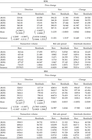
Comparing the (multivariate) Ljung–Box (LB) statistics of the raw with the residual series for the price change direction and the price change size processes in Table 4, shows that both the ACM and the GLARMA models are able to explain a large part of the underlying dynamics very well. However, for IBM, which is the most liquidly traded stock in our sample, the simple ACM(1,1) specification seems unable to capture the dynamic structure completely. A similar picture emerges by comparing the (multivariate) autocorrelograms for the raw with the residual direc-tion and size series. Since there is no new informadirec-tion in these autocorrelograms
at Lancaster University on July 11, 2013
http://jfec.oxfordjournals.org/
Table 3 Estimation results for Coca Cola (KO)
Parameter Model
Price change: Direction ACM model
# Parameters: 16 Estimates Robustt-statistics
µ 1.1789 1.1789 2.2977 2.2977 β1 0.3413 0.5600 0.5600 0.3413 17.653 30.449 30.449 17.653 α1
−0.2755 0.5357 0.5357 −0.2755
−11.916 28.100 28.100 −11.916
γ1
0.4799 −0.6922 −0.6922 0.4799
10.641 −17.414 −17.414 10.641
ζ1=ζV 1ζ1Sζ1D
−0.0738 0.0796 0.0085
−0.0738 0.0796 0.0085
−9.0091 4.0511 0.9074 −9.0091 4.0511 0.9074
ζ2=ζV 2ζ2Sζ2D
−0.0139 0.0098 0.0116
−0.0139 0.0098 0.0116
−1.6861 0.4229 1.2382 −1.6861 0.4229 1.2382
ζ3=ζV 3ζ3Sζ3D
−0.0146 0.0100 0.0184
−0.0146 0.0100 0.0184
−1.8126 0.5236 1.9950 −1.8126 0.5236 1.9950
Price change: Size GLARMA model
# Parameters: 23 Estimates Robustt-statistics ˜
µ −0.0072 −6.6569
˜
β1 0.9981 1638.3
˜
α1 0.0055 6.4415
˜
γ1 0.0055 4.9863
ν0 0.0095 9.3744
ν1 0.0003 2.0814
ν2 0.0003 1.7109
ν3 0.0027 7.4451
ν4 0.0014 5.1365
˜
δ 0.0248 1.4426
˜
ζ1=ζ˜D˜
1, ˜ζ1V, ˜ζ1S, ˜ζ1D
0.0433 0.0594 0.6496 0.0805 2.5143 5.8216 30.577 7.0254 ˜
ζ2=ζ˜D˜
2, ˜ζ2V, ˜ζ2S, ˜ζ2D
0.0208−0.0012 0.0108−0.0076 1.1733−0.1189 0.4502−0.6170 ˜
ζ3=ζ˜D˜
3, ˜ζ3V, ˜ζ3S, ˜ζ3D
0.0242 0.0009 0.0502−0.0295 1.3506 0.0944 2.4628−2.5389
κ−0.5 1.5158 28.958
Transaction volume FIACV model
# Parameters: 18 Estimates Robustt-statistics
µ 0.0423 31.715
β1 0.7985 153.60
α1 −0.0153 −8.0018
ν0 0.1013 31.889
ν1 0.0173 22.651
ν2 0.0095 15.473
ν3 0.0245 25.928
ν4 0.0173 23.381
d 0.1159 51.378
ζ1=ζC 1,ζ1S,ζ1D
−0.0001 0.0757 0.0625 −0.0794 21.665 46.251
ζ2=ζC 2,ζ2S,ζ2D
0.0067−0.0414 0.0198 9.4855−10.426 13.356
ζ3=ζC 3,ζ3S,ζ3D
0.0008−0.0378−0.0107 0.8064−12.762−6.9014 (Continued)
at Lancaster University on July 11, 2013
http://jfec.oxfordjournals.org/
Table 3 (Continued)
Parameter Model
Bid–ask spread FIACS model
# Parameters: 18 Estimates Robustt-statistics
µ 0.1330 8.9947
β1 0.1179 3.3698
α1 0.3948 10.792
ν0 −0.1358 −3.7532
ν1 0.0073 0.6593
ν2 0.0020 0.1869
ν3 −0.0378 −2.4447
ν4 −0.0150 −1.1720
d 0.3157 6.4453
ζ1=ζV 1,ζ1C,ζ1D
0.0296 0.0034 0.0102 7.7483 1.2044 2.3167
ζ2=ζV 2,ζ2C,ζ2D
−0.0014 0.0034−0.0001 −0.3614 1.1775−0.0321
ζ3=ζV 3,ζ3C,ζ3D
−0.0001 0.0020−0.0058 −0.0268 0.5581−1.3161 Intertrade duration
FIACD model
# Parameters: 18 Estimates Robustt-statistics
µ 0.2772 14.195
β1 0.4041 15.222
α1 −0.1706 −18.214
ν0 −0.0019 −0.1098
ν1 −0.0550 −10.655
ν2 0.0110 2.7698
ν3 0.0102 1.4867
ν4 −0.0022 −0.4405
d 0.1677 18.804
ζ1=ζV 1,ζ1S,ζ1C
−0.0430 0.1114 0.0025 −12.458 13.251 1.2250
ζ2=ζV 2,ζ2S,ζ2C
0.0113 0.0503 0.0027 3.0341 4.8096 1.6251
ζ3=ζV 3,ζ3S,ζ3C
0.0143−0.0368−0.0019 4.0697−4.2543−0.7112 Copula function
4-Dimensional Gaussian
# Parameters: 6 Estimates Robustt-statistics
=(ρi j),i,j=C,V,S,D
⎛ ⎜ ⎜ ⎝
1 0.0295−0.1456 0.0334 0.0295 1 0.0577 0.1574 −0.1456 0.0577 1 −0.1727
0.0334 0.1574−0.1727 1
⎞ ⎟ ⎟ ⎠ ⎛ ⎜ ⎜ ⎝
1 6.8352−18.063 5.6428 6.8352 1 7.4651 35.529 −18.063 7.4651 1 −16.996
5.6428 35.529−16.996 1
⎞ ⎟ ⎟ ⎠
in addition to the Ljung–Box statistics, we do not present them here for the price change subprocesses (direction and size); instead we only present the residual au-tocorrelogram of the complete price change process in the first row of Figure 3. Comparing these autocorrelograms with those of the raw series in Figure 1 for all three stocks, demonstrates that the bid–ask bounce effects have been explained by the proposed model specifications.
Let us consider Tables 1–3 again and address the fractionally integrated spec-ifications for the transaction volume, the bid–ask spread, and the intertrade dura-tions. For all three stocks, the fractionally differencing parameterdis smallest for the volume, second smallest for the duration, and largest for the spread process.
at Lancaster University on July 11, 2013
http://jfec.oxfordjournals.org/
Table 4 Model evaluation for Black & Decker (BDK) upper panel, International Business Machines (IBM) middle panel, Coca Cola (KO) lower panel
BDK Price change
Direction Size Change
Raw Residuals Raw Residuals Raw Residuals LB(10) 218.46 60.058 296.22 11.381 15.955 28.520 LB(20) 300.04 99.909 348.38 20.823 30.484 38.570 LB(30) 342.02 132.81 368.70 27.446 34.907 41.658 LB(40) 380.08 173.49 380.03 34.940 41.947 52.311 LB(50) 420.30 213.35 387.31 42.427 46.786 58.275 Mean
0.2963 0.3030
−0.0027 0.0082
3.1235 −0.0003 0.0042 0.0044 Variance
0.2085 −0.0897 −0.0897 0.2112
0.8104 0.0646 0.0646 1.2533
11.021 1.3137 12.449 1.1718 Transaction volume Bid–ask spread Intertrade duration Raw Residuals Raw Residuals Raw Residuals LB(10) 363.64 17.055 9575.2 5.8768 909.24 10.625 LB(20) 425.44 21.400 10882 19.647 1429.6 16.066 LB(30) 464.27 30.668 11471 24.359 1758.1 20.788 LB(40) 472.62 35.249 11710 30.361 2054.7 27.799 LB(50) 477.07 44.947 11867 37.145 2256.9 33.918 Mean 710.03 1.0064 0.0670 1.0072 53.077 0.9813 Variance 2537815 3.9570 0.0029 0.5480 5525.6 1.5751
IBM Price change
Direction Size Change
Raw Residuals Raw Residuals Raw Residuals LB(10) 3260.0 617.19 4280.4 50.870 954.47 57.414 LB(20) 3379.3 681.53 5418.7 58.781 977.38 62.454 LB(30) 3464.4 755.82 6137.6 65.356 1009.8 74.402 LB(40) 3513.2 790.01 6647.8 76.419 1017.4 81.319 LB(50) 3567.5 840.42 7038.7 82.239 1028.2 90.472 Mean
0.3072 0.3277
−0.0089 0.0295
3.5603 0.0015 −0.0052 0.0309 Variance
0.2128 −0.1007 −0.1007 0.2203
0.7803 0.0829 0.0829 1.2980
14.987 1.6244 17.580 1.2620 Transaction volume Bid–ask spread Intertrade duration Raw Residuals Raw Residuals Raw Residuals LB(10) 3599.5 38.732 91591.5 21.322 5016.6 40.528 LB(20) 4896.8 58.703 102299 52.631 8417.3 56.191 LB(30) 5807.5 66.184 109206 66.393 11485 76.715 LB(40) 6419.2 74.193 114782 73.519 14192 86.081 LB(50) 6926.6 82.433 119813 91.328 16728 103.82 Mean 1744.9 1.0263 0.0710 1.0026 6.8712 1.0257 Variance 222993 4.6370 0.0030 0.4456 42.716 0.8251 (Continued)
at Lancaster University on July 11, 2013
http://jfec.oxfordjournals.org/
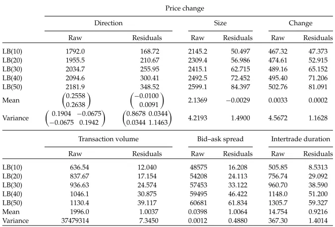
Table 4 (Continued)
KO Price change
Direction Size Change
Raw Residuals Raw Residuals Raw Residuals LB(10) 1792.0 168.72 2145.2 50.497 467.32 47.373 LB(20) 1955.5 210.67 2309.4 56.986 474.61 52.915 LB(30) 2034.7 255.95 2415.1 62.715 489.16 65.152 LB(40) 2094.6 300.41 2492.5 72.452 495.40 71.206 LB(50) 2181.9 348.52 2599.1 84.397 502.76 81.091 Mean
0.2558 0.2638
−0.0100 0.0091
2.1369 −0.0029 0.0033 0.0002 Variance
0.1904 −0.0675 −0.0675 0.1942
0.8678 0.0344 0.0344 1.1463
4.2193 1.4900 4.5672 1.1628 Transaction volume Bid–ask spread Intertrade duration Raw Residuals Raw Residuals Raw Residuals LB(10) 636.54 12.040 48575 16.208 505.85 8.5313 LB(20) 837.67 17.154 54208 24.113 756.74 29.092 LB(30) 936.63 24.574 57453 33.122 960.70 38.590 LB(40) 1046.1 30.875 59495 46.422 1148.0 51.200 LB(50) 1130.4 39.117 60681 61.834 1305.7 59.327 Mean 1996.0 1.0037 0.0398 1.0064 14.754 0.9216 Variance 37479314 7.3450 0.0012 0.4880 367.30 1.4014
∗LB denotes the (multivariate) Ljung Box statistic.
This pattern reflects the different degrees of persistency already depicted by the autocorrelograms in Figure 2. Analyzing the Ljung–Box statistics of the raw and the residual series for these three processes for all three stocks in Table 4 and consider-ing the autocorrelograms of the residual series in Figure 3 (second to fourth row), lead to the conclusion that the fractional integrated model specifications capture the underlying dynamic behavior extremely well.
3.4 Market Microstructure Implications
Market microstructure research analyzes how market participants interact with each other, process information, place orders of a specific size at a certain time and affect the price process within a given institutional framework. Although, theoreti-cal market microstructure models have been available for almost 40 years, Demsetz (1968), Bagehot (1971), and Smidt (1971), for example, attempt to model how mar-ket makers set bid and ask quotes and therefore determine the price process, the availability of high-frequency data sets, and the advances in computer technology have spurred the theoretical and especially the empirical market microstructure research within the last decade. The proposed modeling framework in this paper is not based on an explicit theoretical market microstructure model and the estimated relationships should therefore not be interpreted as structural economic relations.
at Lancaster University on July 11, 2013
http://jfec.oxfordjournals.org/
Figure 3 Residual autocorrelograms of BDK, IBM, and KO price changes (first row), transac-tion volumes (second row), bid-ask spreads (third row) and intertrade duratransac-tions (fourth row). Confidence Bands: Asymptotic 95%.
at Lancaster University on July 11, 2013
http://jfec.oxfordjournals.org/
Nevertheless, our model tries to explain the joint process of four of the most rele-vant market microstructure variables: price changes, transaction volumes, bid–ask spreads, and intertrade durations, and therefore it allows us to investigate how these variables interact with each other and to test well-known implications of theoretical market microstructure models. The use of the copula functions makes the model particularly attractive, since it enables us to analyze the instantaneous relations between our four variables directly and separately from the effects of the lagged explanatory variables (Granger causality relations). This distinction be-tween contemporaneous and lagged effects is often diluted, when implications of market microstructure models are tested with aggregated data. The time scale in our model is defined through the arrival of trades, therefore “instantaneous” refers exactly to the time of a specific trade, which is the highest possible disaggregation level for our data.
The instantaneous causality relations between different market microstructure variables have attracted a lot of attention. Diamond and Verrecchia (1987), Easley and O‘Hara (1992), Dufour and Engle (2000), and Renault and Werker (2006) ex-amine how intertrade duration and return volatilities interact. Whereas, the first three papers postulate an a priori causality relationship from duration to volatil-ity, Renault and Werker (2006) take a structural approach to identify and quantify instantaneous effects in addition to Granger causality effects. Diamond and Ver-recchia (1987) hypothesize, assuming that short selling is prohibited, that bad news are reflected by longer durations which should cause negative price reactions and increasing volatility. Contrarily, Easley and O‘Hara (1992) and Dufour and Engle (2000) consider smaller durations as a sign for a larger share of informed investors being active in the market, which is anticipated by less informed traders and thus causes more uncertainty and therefore higher volatility. The latter point of view has also been confirmed by Engle (2000) as well as by Renault and Werker (2006) for the instantaneous relation between durations and volatility.
Another strand of the literature focuses on the relationship between trading volume and the bid–ask spread. In the early inventory models, see Demsetz (1968) for example, the market maker is seen as providing a service for which he has to be compensated by letting him earn the bid–ask spread. Smidt (1971), Garman (1976), Stoll (1978), Ho and Stoll (1981), Hasbrouck and Sofianos (1993), and Madhavan and Smidt (1993), however, assume that the market maker, who might be allowed to trade actively in the market on his own account, holds an optimal inventory and deviations from this optimal inventory, induced by large trades, cause an inventory risk which is mirrored into the bid–ask spread. A different explanation for the connection between transaction volumes and bid–ask spreads is given by asymmetric information based models, see Bagehot (1971), Copeland and Galai (1983), Glosten and Milgrom (1985), or Easley and O’Hara (1987). In these models the market maker is assumed to make profits when trading with uninformed investors and assumed to make losses when trading with informed investors. Thus, based on historical order flow, which includes trading speed and trading volume, the market maker tries to figure out whether he faces an informed investor, which would force him to increase the bid–ask spread.
at Lancaster University on July 11, 2013
http://jfec.oxfordjournals.org/
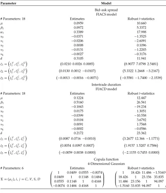
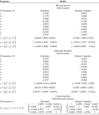
Let us consider Tables 1–3 again and examine the instantaneous effects among our variables captured by the copula parametersρi j,i,j = {C,V,S,D}, as well as
the Granger causality effects represented by the parameters of the lagged explana-tory variables ζi. For all three stocks, the copula parameter ρVS is significantly
positive, representing a positive instantaneous relationship between transaction volume and bid–ask spread. Moreover, within the FIACS model, we observe for all three stocks only significant positive parametersζV
i ,i =1, . . . , 3, reflecting that
higher trading volumes Granger cause higher bid–ask spreads. These observations are clearly in line with the findings from the inventory and asymmetric information models cited above.
The effect of time on the bid–ask spread and on the price change volatility, which is modeled by the GLARMA specification is not that clear-cut but shows an interesting pattern. First of all, the instantaneous effect between intertrade duration and the bid–ask spread,ρSD, is negative for BDK and KO but positive for IBM,
which means that a higher trading intensity (smaller durations) is accompanied by a higher bid–ask spread for BDK and KO, but by a smaller one for IBM. Moreover, in the FIACS model,ζ1Dis also significantly negative for BDK strengthening the instantaneous effect, positive for KO compensating the instantaneous effect and positive for IBM supporting the instantaneous effect, which is then weakened by
ζD
2 andζ3D, which are significantly negative.
These ambiguous effects (especially the instantaneous ones) between dura-tions and the bid–ask spread can be interpreted in the light of the theoretical mod-els of Admati and Pfleiderer (1988) and Foster and Viswanathan (1990). Whereas, in the model of Admati and Pfleiderer (1988) both informed and uninformed in-vestors have a high incentive to trade and therefore a high trading intensity when trading costs are low, Foster and Viswanathan (1990) assume that high trading intensity is only caused by informed investors, preventing uninformed investors from trading at these times and causing higher bid–ask spreads being set by the market maker. Our results do not allow us to favor one of these models when the instantaneous effect between duration and bid–ask spread is examined. However, the Granger causality effects of the bid–ask spread on durations (ζiSi=1, . . . , 3 in the FIACS model) show that for all three stocks a higher bid–ask spread at the previous trades leads to increasing intertrade durations and thus to lower trading activity. This observation supports the Admati and Pfleiderer (1988) model. Inter-preting the Foster and Viswanathan (1990) model in the Granger causality sense, we can still not find support for this model since, as mentioned above, also the lagged effects of durations on the bid–ask spread are indistinct and seem to be dominated by the effects of trading volume.
The ambiguity of the effect from durations on the bid–ask spreads can be combined with the observation that for all three stocks, price change volatil-ity (GLARMA model) is significantly increasing in lagged trading volumes ( ˜ζV
i ,
i=1, . . . , 3) and lagged bid–ask spreads ( ˜ζS
i,i=1, . . . , 3), but again there is no
clear influence of lagged durations on volatility. Furthermore, we also observe no clear effect of instantaneous (ρV D) and lagged durations (ζiD,i =1, . . . , 3) on
transaction volume (FIACV model) for all three stocks. Taking these observations
at Lancaster University on July 11, 2013
http://jfec.oxfordjournals.org/