Analytical framework for Adaptive Compressive Sensing for Target Detection within Wireless Visual Sensor Networks

(will be inserted by the editor)

Analytical framework for Adaptive Compressive

Sensing for Target Detection within Wireless Visual

Sensor Networks

Salema Fayed · Sherin M.Youssef ·

Amr El-Helw · Mohammad Patwary ·

Mansour Moniri

Received: date / Accepted: date

Abstract Wireless visual sensor networks (WVSNs) are composed of a large number of visual sensor nodes covering a specific geographical region. This pa-per addresses the target detection problem within WVSNs where visual sensor nodes are left unattended for long-term deployment. As battery energy is a critical issue it is always challenging to maximize the network’s lifetime. In order to reduce energy consumption, nodes undergo cycles of active-sleep pe-riods that save their battery energy by switching sensor nodes ON and OFF, according to predefined duty cycles. Moreover, adaptive compressive sensing is expected to dynamically reduce the size of transmitted data through the wireless channel, saving communication bandwidth and consequently saving energy. This paper derives for the first time an analytical framework for select-ing node’s duty cycles and dynamically choosselect-ing the appropriate compression rates for the captured images and videos based on their sparsity nature. This reduces energy waste by reaching the maximum compression rate for each dataset without compromising the probability of detection. Experiments were conducted on different standard datasets resembling different scenes; indoor and outdoor, for single and multiple targets detection. Moreover, datasets were chosen with different sparsity levels to investigate the effect of sparsity on the compression rates. Results showed that by selecting duty cycles and dynam-ically choosing the appropriate compression rates, the desired performance

S. Fayeda∗·S. M.Youssefa·A. El-Helwb

a_{Computer Engineering Department,}b_{Electronics and Communication Department,}

College of Engineering and Technology, AAST, Alexandria, Egypt * E-mail: [email protected]

M.Patwaryc

c_{School of Computing and Digital Technology, Birmingham city University}

Birmingham, B47XG UK

M. Monirid

d_{School of Architecture, Computing and Engineering, University of East London,}

of detection can be achieved with adaptive CS and at the same time saving energy, where the proposed framework results in an 70% on average energy saving as compared to transmitting the captured image without CS.

Keywords Compressive sensing·Duty cycles ·Target detection ·Wireless visual sensor networks

1 Introduction

Due to the advancement of new technologies, there are immediate requirements for automated energy-efficient Wireless Visual Sensor Networks (WVSNs) ap-plications. WVSNs have addressed various applications such as environmental monitoring, animal behavior, surveillance applications, law enforcement, in-dustrial automation and military purposes. Visual sensor nodes are resource constraint devices bringing together the special characteristics of WVSNs such as energy, storage and bandwidth constraints that introduced new chal-lenges [1–6]. Each visual sensor node is powered by an attached battery and embeds a visual sensor, digital signal processing unit, limited memory and a wireless transceiver. The visual sensor can be integrated with other types of sensors such as vibration and acoustic sensors. Energy utilization is neces-sary to maximize the network’s lifetime due to the limited battery power and communication bandwidth.

This paper addresses the target detection problem within WVSNs where visual sensor nodes are left unattended for long-term deployment. Amongst the many diverse application domains of WSNs, object detection is one of the most important tasks in image processing applications. Object can be a human being, a vehicle or any targeted object. As battery energy is a critical issue, it is always challenging to maximize the network’s lifetime by minimizing the energy consumption due to sensing, processing and transmission without com-promising the detection performance. In order to reduce energy consumption, nodes undergo cycles of active-sleep periods that save their battery energy by switching sensor nodes ON and OFF, according to a predefined duty cycles.

energy, memory constraints and communication bandwidth, CS will not af-fect quality of image (as denoted by Peak signal-to-noise ratio (PSNR)) for later target detection. Adaptive CS dynamically chooses the compression rate according to the sparsity nature of frames that varies from one dataset to an-other. In contrast to static compression rates, different datasets have different sparsity levels, hence if the same dimension of the sensing measurement ma-trix is used for more sparse images, this will result in a waste of energy where more compression could have been applied. In the case of less sparse images, the quality after reconstruction will be affected. Therefore, dynamic size of sensing measurement matrices result in saving energy, space requirements, as well as channel bandwidth.

Due to many factors such as node deployment, number of nodes, velocity and position of targets, the performance of detection may degrade. Moreover, the impact of CS versus adaptive CS to reduce the size of transmitted data on the object detection problem for WVSNs is analyzed. As a result of integrating adaptive CS with the detection problem, the performance may feature further degradation than the desired and acceptable performance level. This is due to other factors such as image sparsity and, loss of information in compression. Hence, there is always a tradeoff between energy consumption (network life-time) and detection performance. As a result, the main goal of this paper is to derive an analytical framework to examine the selection of sensor node’s duty cycles and dynamically choosing compression rates for different images and videos. The idea is to maximize the network’s lifetime and reduce the energy waste without compromising the probability of detection.

The rest of the paper is organized as follows, related work is discussed in Section 2. Introduction to CS is then presented in Section 3. Section 4 presents the proposed system model. The analytical framework is first derived in Section 5 to evaluate the probability of missed detection, then the impact of adaptive CS on the probability of missed detection is investigated. Simulations and results are presented and discussed in Section 6. Finally the conclusion and future work are summarized in Section 7.

2 Related work

duty cycle period and the percentage of time nodes are awake within each duty cycle. However, the wake-up times are not synchronized among nodes as random scheduling is probably the easiest to implement in sensor networks, since it requires no coordination among nodes. Moreover, coordination among nodes requires additional energy as it involves some message exchange. In con-trast, random scheduling does not require communication, each node simply sets its own duty-cycle schedule according to the agreed-upon wakeup ratio. The authors derived an analytical framework for the detection problem under different parameters such as duty cycles, nodes sensing times and number of deployed nodes.

A node selection scheme is presented in [9], which gives full consideration to both the information utility for the quality of tracking and the remaining energy of nodes to determine the longetivity of nodes. Each sensor node is responsible of computing the detection probability, whereas the optimal set of sensors perform target tracking by integrating partial estimations. The node selection is formalized as an optimization problem and solved by genetic al-gorithms to optimize the tradeoff between the accuracy of tracking and the energy cost of nodes. While in [10] energy conservation in target tracking is achieved using different methods, prediction-based scheme coupled with selec-tive activation of nodes is one of such methods, where nodes are waked-up on-demand following the target path. Previous active nodes collaborate be-tween each other to generate an accurate estimation of the target.

In [11], the authors integrated reactive mobility of sensor nodes to improve the target detection performance of WSNs. Sparsely deployed mobile sensors collaborate with static sensors and move in a reactive manner to achieve the required detection performance. Specifically, mobile sensors remain stationary until a possible target is detected.

In the context of CS, it is a useful imaging tool under various noise con-ditions when the underlying image is compressible in a known basis or repre-sentation. CS is a new paradigm for data acquisition and processing originally developed for the efficient storage and compression of digital images [12, 13], it has been widely used in several applications such as image processing, steganography and image watermarking [14, 15]. In [16], compressive sensing for background subtraction and multi-view ground plane target tracking are proposed. A convex optimization known as basis pursuit or orthogonal match-ing pursuit is exploited to recover only the target in the difference image usmatch-ing the compressive measurements to eliminate the requirement of any auxiliary image reconstruction. Other work in compressive sensing for surveillance ap-plications has been proposed in [17], where an image is projected on a set of random sensing basis yielding some measurements, where at the receiver end the image is reconstructed by minimizing the weighted version of the L2 norm. However, further research is required to address the selection of the weights and fully understand their impact on the reconstruction problem while taking into account the energy-efficiency parameter.

An adaptive approach is proposed to select a routing path by choosing sen-sors required to transmit their data. However, in this approach adaptive CS is only applied for sensor nodes selection and no compression is performed on the transmitted data. A heuristic to solve the optimization problem (which is proven NP-hard) is proposed in [19] to find a sensing measurement matrix that maximizes the information gain per energy expenditure. It was shown that under suitable conditions, one can reconstruct an (N×N) matrix of rank

rfrom a small number of its sampled measurements. This is done by solving an optimization problem, provided that the number of measurements is of order

N1.2r_{logn, exact matrix recovery would be guaranteed with a reduced number} of measurements. Subsequently, most existing work in adaptive compressive sensing use heuristic techniques which are computationally expensive, hence taking only into consideration the accuracy of the approximate data field while relaxing the energy constraint.

In [20], an adaptive block CS technique is proposed and implemented to represent the high volume of captured images for the purpose of energy effi-cient wireless transmission and minimum storage. Adaptive CS is expected to dynamically achieve higher compression rates depending on the sparsity na-ture of different datasets, while only compressing relative blocks in the image that contain the target to be tracked instead of compressing the whole image. Hence, saving power and increasing compression rates. Least mean square adaptive filter is used to predict the next location of the target to investigate the effect of CS on the tracking performance. The tracking is achieved in both indoor and outdoor environments for single/multi targets. Experiments were carried out to evaluate the performance of the adaptive CS and its effect on target detection and tracking. Results have shown that using adaptive CS, up to 20% measurements of data are required to be transmitted while preserving image quality. Moreover, for different datasets where the sparsity nature of each image differs, CS adaptively chooses the compression rates accordingly reaching a relation between the number of compressed measurements and ratio of non-zero pixels to the total number of pixels.

problem and considering the resource constraints within WVSNs for target detection to evaluate the impact of energy saving due to visual sensor nodes’ duty cycles. Moreover, to show that by choosing appropriate compression rates according to different sparsity levels of images, one can keep the same level of detection while reducing the size of transmitted images through the wireless channel which as a result increases the network’s lifetime by saving energy that is one of the main constraints of wireless visual sensor networks (WVSN).

3 Compressive Sensing

According to Shannon-Nyquist sampling theory the minimum number of sam-ples required to accurately reconstruct the signal without loss is twice its max-imum frequency [21]. It is always challenging to reduce this sampling rate as much as possible, hence reducing the computation energy and storage. Within the scope of the authors knowledge, recently proposed CS [21] is expected to be a strong candidate to provide this and overcome the above mentioned limitations, where CS has been considered for different aspects of surveillance applications due to its energy efficient and low power processing as reported in [16, 22]. CS theory shows that a signal can be reconstructed from far fewer samples than required by Nyquist theory, provided that the signal is sparse (where most of the signal’s energy is concentrated in few non-zero coefficients) or compressible in some basis domain [23]. CS is a simple and low energy con-sumption process which is suitable for power constraint sensor nodes, where complex computations are just done at the Base station (BS).

CS exploits the sparsity nature of frames, so it compresses the image us-ing far fewer measurements. Although, it is not necessary for the signal itself to be sparse but compressible or sparse in some known transform domain Ψ

according to the nature of the image (i.e., the original image has approxi-mate sparse representations in some linear transformations), smooth signals are sparse in the Fourier basis, and piecewise smooth signals are sparse in a wavelet basis [12, 23–25].

Suppose an image’X’of size (N×N) is K-sparse (where K is the number of non-zero elements) that either sparse by nature or sparse in some domain namedΨdomain, whereΨis the basis invertible Orthonormal function of size (N×N) used to sparsify the image, driven from some transform such as the DCT, fourier, or wavelet, whereKN, that is, only K coefficients of Xare nonzero and the remaining are zero, thus the K-sparse imageX is compress-ible. CS then guarantees acceptable reconstruction and recovery of the image from lower number of samples (known as measurements) as compared to those required by shannon-Nyquist theory as long as the number of measurements

M satisfies a lower bound defined in Eq.(1) which depends on how sparse the image is. Eq.(2) shows the mathematical representation ofX.

X=ΨS (2) Where,Sis a matrix containing the sparse coefficients ofXof size (N×N), The image is represented with fewer samples fromX instead of all pixels by computing the inner product betweenXand a random sensing matrix known as Φ, namely through incoherent measurements Y in Eq.(3), where Φ is of size (M ×N) whereK << M << N.

y1 =< x,φ1 >, y2 =< x, φ2 >,· · · ,ym =< x, φm >. Where φ1, φ2· · ·φm

represent individual rows inφ

Y=ΦX=ΦΨS=ΘS (3)

Since M < N, recovery of the image Xfrom the measurements Y is un-determined, However, if Sis K-sparse, and M ≥KlogN it has been shown in [23] thatXcan be reconstructed by`1norm minimization with high

proba-bility through the use of special convex optimization techniques without having any knowledge about the number of nonzero coefficients ofX, their locations, neither their amplitudes which are assumed to be completely unknown a pri-ori [12, 25, 26]

minkXˆk`1 subject to Φ ˆX=Y (4)

Convex optimization problem can be reduced to linear programming known as Orthogonal Matching Pursuit (OMP) which was proposed in [27] to handle the signal recovery problem. It is an attractive alternative to Basis Persuit (BP) [13] for signal recovery problems. The major advantages of this algorithm are its speed and its ease of implementation. As seen, the CS is a very simple process as it enables simple computations at the encoder side (sensor nodes) and all the complex computations for recovery of frames are left at the decoder side or BS.

4 WVSN model

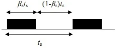
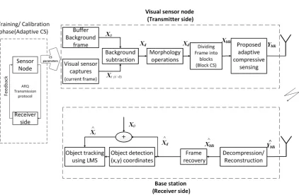
Consider a WVSN-based surveillance application model, composed ofNvisual sensor nodes randomly distributed over a specific geographical region as in Fig.1. Each sensor node is assumed to have a sensing radius rs allocated to share a viewable range and fully cover the required geographical region, and one or more receiver/sink node at fusion center. The geographical region is assumed to be a square area with each side of sizeds. It is required to increase the WVSN’s lifetime by reducing the energy consumption this is accomplished by periodically switching On and OFF the visual sensors. Each sensor node is assumed to be in ’wake-up’ state according to a duty cycle βs ∈[0,1] over a periodts, hence each sensor is awake for an interval of lengthβsts and sleep for an interval (1−βs)ts as shown in Fig,2.

Fig. 1 Wireless visual sensor network

Fig. 2 Scheme for sensor’s duty cycle

detection performance presented in [8]. Lets assume the following, the time reference for the frame count is assumed to bet= 0. Hence, a single snapshot at t = 0 is expected to be stored within the memory allocated at the sensor node; that is assumed to be the background for the intended target detection; will be denoted asXb. Following framesXt witht >0 are subsequently

cap-tured frames in the video sequence, where Xb and Xt are of size (N ×N).

To achieve higher compression rates, the foreground target is extracted first by background subtraction resulting in the difference frameXd. Hence,

assur-ing sparsity as the difference frame is always sparse regardless of the sparsity nature of original image frames. Within the image frame, the extraction of foreground target Xd is achieved at each sensor node, where CS is then

ap-plied producing the compressed measurements Yd for transmission through

the wireless channel.

is used for all different datasets, for more sparse images this will result in a waste of energy, where more compression rates could have been applied. And for less sparse images, the quality after reconstruction will be affected which in return degrades the detection performance. As a result, dynamic size of sensing measurement matrices result in saving energy, space requirements, as well as channel bandwidth. It is expected that the reliability of target detection will be different as the degree of sparsity varies from one image to another, for this reason there is a great challenge for adaptive CS by making the dimension of M variable depending on how sparse the image is. For the adaptive CS, the traditional CS process is preceded by a calibration phase. During that phase an Automatic Repeat Query (ARQ) transmission protocol is used between sensor nodes and the receiver side, as feedback is needed for the adaptation phase. A dictionary is constructed for different values of M

and corresponding sensing matrices Φ. For each dataset the sparsity level is calculated by finding the ratio between the number of non-zero pixels and the total number of pixels in a frame. At the end of each adaptation/calibration phase, the dictionary is updated with the chosenM andΦfor the equivalent sparsity level that can be used later for other datasets with the same sparsity levels. Initially, an arbitrary value of M is chosen according to a sparsity measure and is used to obtain the compressed measurementsYd. The sensor

node is then set to transmit Yd to the receiver side, where the image is to

be reconstructed, and based on the reconstruction mean square error which is used as a performance indicator, a decision is made whether the reconstruction is satisfactory or not. In case the reconstruction results are satisfactory, the receiver node sends a ’zero’ flag through the feedback channel, ending the calibration phase; otherwise a ’one’ flag is to be sent. While the sensor node receives a ’one’ flag, it is expected to change the value of M and change Φ

accordingly, the sensor node repeats the search for an optimum value ofM at the CS adaptation process till it receives a zero feedback from the receiver. At this point, the optimum values forM andΦobtained are used next in the CS process.

At the receiver side, the received compressed data is to be decompressed for the reconstruction and recovery of the estimated dataXˆd. As mentioned,

Xb is known to the receiver making it possible to estimate and reconstruct

the original test frame denoted as Xˆt by adding Xb after masking the

tar-get’s locations in the background image to Xˆd. Finally, the system detects

moving targets. The system model of the proposed work for the WVSN-based surveillance application is shown in Fig.3.

Fig. 3 The proposed model for WVSN-based surveillance application

5 Probability of missed detection

In subsequent sections an analytical framework is derived, first to evaluate the probability of missed detection as a function of the target’s mobility model due to the predefined duty cycles. Second, the probability of missed detection is derived after the integration of adaptive CS to compare the performance of detection with and without CS.

5.1 Probability of missed detection as a function of mobility model of the target

In order to detect a target in a squared geographical area, N sensors are randomly deployed and set to periodically switch ON and OFF according to a predefined duty cycle βs. To evaluate the probability of missed detection

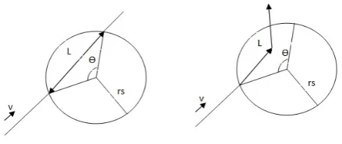
Pmd, it is required to integrate the sensor’s duty cycle. Assume that the target enters the sensing area at timetawith angleθand velocityv m/scrossing the sensing area inTcross=L/vwhereLis the length of intersection between the target’s trajectory and the sensing arearsas shown below in Fig.4,

Fig. 4 Sensor model for (a) linear and (b) non-linear target trajectory

geographical area, N visual sensor nodes are distributed to cover this area. So,

ξtarget describes the presence of a target in the required sensing area at the

time where a given sensor is ON.ξdetis the event where the sensor is ON when the target crosses the sensor’s sensing area, so the target is detected by the given sensor. During a single time interval ts, any incoming target entering a sensor’s sensing area at time Ta during the interval βsts (i.e. the sensor is ON) will be detected. However, in the case whereTa is during the interval (1−βs)ts(i.e. during the sensor’s sleep interval), in order to successfully detect the target, the target must remain in the sensing area till the sensor’s next duty cycle where it turns ON again. Hence, the Probability of detectionPd is defined as in [8] by the total probability theorem as:

Pd=P{ξdet|ξtarget}P{ξtarget}+P{ξdet|ξtarget}P{ξtarget} (5)

Where,P{ξdet|ξtarget}= 1,P{ξtarget}=βs, andP{ξtarget}= (1−βs), the last term P{ξdet|ξtarget} in (5) denotes the case where the target is detected given it enters the sensing area during the sensor’s sleep interval (1−βs)ts. This suggests that either the target’s crossing time Tcross >(1−βs)ts, as a result, the target is detected, or the case whereTcross<(1−βs)ts, in this case the target will only be detected if it enters the sensing area during the last part of the sleep interval, such that the target remains in the sensing area till the sensor turns ON in the next duty cycle. Hence, as in [8]P{ξdet|ξtarget}is calculated in terms of the joint probability density function (pdf) as follows:

P{ξdet|ξtarget}=

Z Z

D

f TaTcross(t, τ)dtdτ (6)

where D is the integration domain described in [8, 28], f TaTcross(t, τ) is the probability density function expressed as:

f TaTcross(t, τ) =

( v

Πc√r2

s−(vτ2)2

if 0< τ <2rs/v, 0< t < c

whereΠ ≈3.14159 andc= (1−βs)tsis the time interval where the target enters the sensing area, hence:

P{ξdet|ξtarget}=

(4rs

πcv if 2rs/v < c

4rs−2

√

4r2

s−c2v2

πcv + 1−

2 arcsin(cv

2rs)

π else

(8)

Finally, thePdis written as:

Pd =βs+ (1−βs)P{ξdet|ξtarget} (9)

Taking into consideration the independence of the N randomly deployed sensor nodes, the probability of missed detection can then be evaluated as:

Pmd= (1−Pd)N (10)

Pmd= (1−[βs+ (1−βs)P{ξdet|ξtarget}])

N ₍₁₁₎

5.2 Probability of missed detection as a function of Compressive Sensing

Integrating CS to reduce the size of transmitted information to the target detection problem might lower the detection performance, as M the size of compressed measurements must be M ≥ Klog(N/K), where, the captured image is (N×N) and K is the number of non-zero pixels (which defines the sparsity level of the image). Hence, if M is chosen according to this bound the target will be detected with high probability. Moreover the performance of the detection problem is directly proportional to the PSNR of the image after reconstruction. First, probability of detection using CSPdcsis calculated

subject to the constraint that the probability of false alarm PF A ≤ α as in [29, 30].

Pdcs=Q(Q

−1_(α)−p

M/N√P SN R/pK/N) (12)

Where,Q(x)_,R∞

x e

−t2_/2

dtis the complementary error function ofx. This gives a way to measure how much information is lost after the reconstruction, not in terms of the reconstruction error of the image, but in terms of the ability to detect the target. To reach an acceptable Pdcs, Φ is dynamically chosen according the sparsity nature of the image but without relaxing the randomness property of the projection sensing measurement matrix. Thus the size ofΦ(MxN) will be adaptively changing with respect toK.

Afterwards, the total probability of detection will be evaluated by inte-grating adaptive CS to the detection problem. Hence, the total probability of detectionPdt becomes as follows:

Pdt = (βs+ (1−βs)P{ξdet|ξtarget})Pdcs (13)

PmdCS = (1−[(βs+ (1−βs)P{ξdet|ξtarget})Pdcs])

N ₍₁₄₎

To maintain a high probability of detectionPdtand a required PSNR while

given the target’s velocity, sparsity level of the image and sensing radius. One can dynamically find the best value forM that suits these requirements as in (16) by solving the following:

ˆ

Pdcs=

( P_dt4dsπcv

(2πrs)(βsπcv)+4rs−4rsβs if 2rs/v < c

P_dt4ds

2πrsZ else

(15)

WhereZ =βs+ (1−βs)(

4rs−2

√

4r2

s−c2v2

πcv + 1−

2 arcsin(cv

2rs)

π )

M =(Q

−1_(α)−Q−1_{( ˆP}

dcs))

2_k

P SN R (16)

5.3 Probability of missed detection for multi-target detection scenario

The analysis of the detection problem is extended to consider the case of multiple targets entering the monitoring area. In this case it will be useful to evaluate the probability of missing all targets or missing at least one of the incoming targets. AssumeNT is the number of incoming targets and the probability of missing all incoming targets is denoted as Pma and since the incoming targets are independent, then it can be evaluated as follows:

Pma= (PmdCS)

NT ₍₁₇₎

Where PmdCS is the probability of missed detection in the case of single

target detection after the integration of CS. The probability of missing at least one of theNT, denoted asPmois expressed as

Pmo= 1−(1−PmdCS)

NT ₍₁₈₎

6 Analysis and discussion

6.1 Duty cycle analysis

The performance of the duty-cycled WVSN is characterized in terms of prob-ability of missed target detection. The effect of different values of βs are ex-amined by testing the probability of detecting a given target as changing the value ofβsis expected to affect the detection problem, whenβsbecomes small, the target can cross the sensed area, during a sleeping interval of a sensor re-sulting in missing a target. The detection performance has been tested under several parameters; different values of sensing timests, duty cyclesβs, sensing areas and number of sensor nodesN. All sensors are assumed to have the same sensing area rs, and targets enter the monitored area with the same velocity

0.2 0.3 0.4 0.5 0.6 0.7 0.8 0.9 1 0

0.1 0.2 0.3 0.4 0.5 0.6 0.7

Bs

Pmd

rs=20 m rs=35 m rs=50 m

(a)

0.2 0.3 0.4 0.5 0.6 0.7 0.8 0.9 1 0

0.05 0.1 0.15 0.2 0.25 0.3 0.35

B_s

Pmd

ts=5 ts=15 ts=25

(b)

0.2 0.3 0.4 0.5 0.6 0.7 0.8 0.9 1 0

0.1 0.2 0.3 0.4 0.5 0.6 0.7 0.8 0.9

Bs

Pmd

N=5 N=20 N=35 N=50

(c)

Fig. 5 Probability of missed detection vs. different duty cycles for (a) different rs (ts =

15sec,N= 50), (b)differentts(N= 50,rs= 50) and (c) different number of sensor nodes

(ts= 15sec,rs= 50). In all cases the target enters with velocityv= 15m/s

6.2 Analysis of Probability of missed detection for duty-cycled WVSN

Analysis are carried out to address the target detection problem after applying sensors duty cycles and to evaluate the probability of missing a target under various parameters;ts, βs, sensing areas and number of sensor nodesN.

Fig.5 shows the Pmd as a function of βs for various values of rs, ts and sensor nodes N, in all cases the target’s velocity is 15m/s. As illustrated, for lower values of βs, there is a high chance the target enters and crosses the sensed area during the sleeping interval of the sensor, resulting in higher probability of missed detection. Asβs increases, the sensor node stays on for a longer time, decreasing the probability of missing a target. In Fig.5(a), the

As shown, for larger sensing areas, the higher the probability of detecting the incoming target.

In Fig.5(b), Pmd is shown for different values of ts, while rs and N are set to 50. It is clear from the figure that for lower values ofts, the lower the probability of missed detection and the lower the impact ofβson the detection problem, where the total sensing periodtsis short and sensors switch to the ON state more often. While for longerts,βshas a direct impact on the probability of missing a target, asβsbecomes small, the probability a target crosses the sensing area while the sensor is in the OFF state gets higher leading to a higherPmd. In contrast, whenβsapproaches 1 (sensors remain ON), thePmd converges for different values of ts as the effect of ts on the probability of detecting a target becomes negligible.

The impact of different numbers of sensor nodes on Pmd is illustrated in Fig.5(c), wherets is set to 15secand rs to 50. As shown, asN increases, the

Pmddecreases which explains that by deploying more sensors in the monitoring geographical area the higher the chance to guarantee more sensing coverage hence reducing the probability a target is missed. On the other hand, if fewer sensors are deployed, the probability a target enters a non-coverage area is high, as a result the probability the target is missed is higher. Fig.6 shows the

Pmdas a function ofβsforN = 1 and different values ofrs, there is significant increase in Pmd >90% even the effect of increasing the sensing area on the target detection problem becomes significantly low.

0.2 0.3 0.4 0.5 0.6 0.7 0.8 0.9 1 0.92

0.93 0.94 0.95 0.96 0.97 0.98 0.99 1

Bs

Pmd

rs=20 rs=35 rs=50

Fig. 6 Probability of missed detection vs. different duty cycles forN= 1 and differentrs,

ts=15sec and the target enters with velocityv= 15m/s

Another important parameter that has a direct impact onPmdis the tar-get’s velocity when crossing the sensing area which in return also affects the time required by the target to cross a given sensing areaTcross. In Fig.7,Pmd is analyzed as a function ofβsfor different values ofvwhile other parameters are kept constant (N = 50,ts= 15sec, rs= 50). For small values ofβs (the sensor is ON for short intervals) there is a high impact of v onPmd, where

the sensing areaTcrossand as a result the target might cross the sensing area during a sensor’s sleeping interval hence resulting in higherPmd. On the other hand, for lower velocities, the target crosses the sensing area for Tcross long enough so that any sensor on the target’s trajectory will detect it even if the sensor is in sleeping mode when the target enters its sensing area, there will be a high probability the sensor turns ON before the target leaves its sens-ing area. As βs approaches 1, target’s velocityv has a limited impact on the detection performance andPmd converges to reach a lower bound.

0.2 0.3 0.4 0.5 0.6 0.7 0.8 0.9 1 0

0.05 0.1 0.15 0.2 0.25

Bs

Pmd

v=0 v=5 v=10 v=15

Fig. 7 Probability of missed detection vs. different duty cycles for different target’s velocity (N= 50,rs= 50,ts= 15sec)

Fig.8 shows the Pmd as a function ofβs for various values ofrsand v set to 100m/s, N to 50 andtsto 15sec. As stated above, higher velocities result in higher probability of missing a target specially during shortβsduty cycles as the target crosses the sensing area in a short interval of time (the case where the sensor is OFF when target enters a sensing area and target leaves the sensing area before the sensor turns On again). However, the impact of high velocities could be eliminated by longerβsand largerrs, to increase the probability the target remains in the sensing area for a longer interval of time till detected. This is reflected in the figure, where for a 100m/svelocity the

Pmddecreases asrs andβsincreases.

6.3 CS Simulation

0.2 0.3 0.4 0.5 0.6 0.7 0.8 0.9 1 0.1

0.2 0.3 0.4 0.5 0.6 0.7 0.8 0.9 1

Bs

Pmd

rs=10 rs=25 rs=40

Fig. 8 Probability of missed detection vs. different duty cycles for differentrs, v=100m/s,

ts= 15sec, N=50

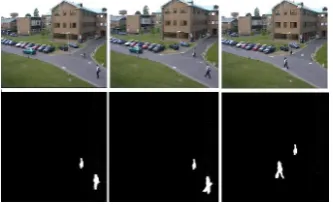
standard datasets chosen with different sparsity levels to investigate the effect of sparsity on the compression rates and how dynamically compression rates are selected to evaluate the performance of adaptive CS by choosing appro-priate compression rates depending on sparsity nature of images; ”Walking men” is chosen for dataset”1” to resemble an outdoor scene for multi target captured by [31]. While ”Shopping center 1” and ”Shopping center 2” for in-door scenes with different sparsity levels, tracking a single target from two different views; top view with a wide angle lens camera and a corridor side view, for dataset”2” and dataset”3” respectively, filmed for the EC funded CAVIAR project (CAVIAR is a project of the European Commission’s Infor-mation Society Technology program found in [32]). ”Walking” for dataset”4” resembles an outdoor scene with a street view for cars and targets tracking from PETS surveillance datasets [33], and according to the application, spe-cific objects (cars or pedestrians) will be detected. Fig.9 shows samples from different datasets and the corresponding detected target. Next, we show the probability of detection by applying CS for various compression rates. Then, the impact of CS on the total probability of missed detection is illustrated.

(a) dataset ”1” Walking Men (b) dataset ”2” Shopping center 1

(c) dataset ”3” Shopping center 2

(d) dataset ”4” Walking

Fig. 9 First row in (a)(b) (c) and (d) shows test frames from different datasets and detected targets in second row

entries are either +1 or -1 and whose rows are mutually orthogonal, the matrix is first randomly reordered then,M samples are randomly chosen to construct the (M×N) random sensing matrixΦ.

6.3.1 Target Detection

30 40 50 60 70 80 90 0 200 400 600 800 1000 1200 1400

Number of CS measurements M

Reconstruction MSE

Average reconstruction MSE vs. M

CS using randn CS using hadamard

(a) Reconstruction MSE

30 40 50 60 70 80 90

15 20 25 30 35 40

Number of CS measurements M

Average PSNR

Average PSNR of reconstructed difference images vs. M

CS using randn CS using hadamard

(b) PSNR

Fig. 10 Comparing reconstruction MSE and PSNR using randn and walsh sensing matrices for ”Walking men” with K=30%

10 20 30 40 50

0 10 20 30 40 50

Number of CS measurements M

Reconstruction MSE

Average reconstruction MSE vs. M

CS using randn CS using hadamard

(a) Reconstruction MSE

10 20 30 40 50

24 26 28 30 32 34

Number of CS measurements M

Average PSNR

Average PSNR of reconstructed difference images vs. M

Randn hadamard

(b) PSNR

Fig. 11 Comparing reconstruction MSE and PSNR using randn and walsh sensing matrices for ”Shopping center 1” with K=3%

that for different sparsity levelsK= 30%,3% and 11% respectively, different values ofMand compression rates are required. When reaching optimum value of M, least MSE and 33dB PSNR are successfully achieved. For illustration, MSE decreases and PSNR increases asM increases till reaching the optimum value, it has been shown that the lower bound on M is dependent on how sparse the difference frame Xd is or in other words proportional to the ratio

20 30 40 50 60 0

2 4 6 8 10 12 14

Number of CS measurements M

Reconsruction MSE

Average Squared error of reconstructed difference images vs. M

CS using randn CS using hadamard

(a) Reconstruction MSE

20 30 40 50 60

26 28 30 32 34 36

Number of CS measurements M

Average PSNR

Average PSNR of reconstructed difference images vs. M

CS using randn CS using hadamard

(b) PSNR

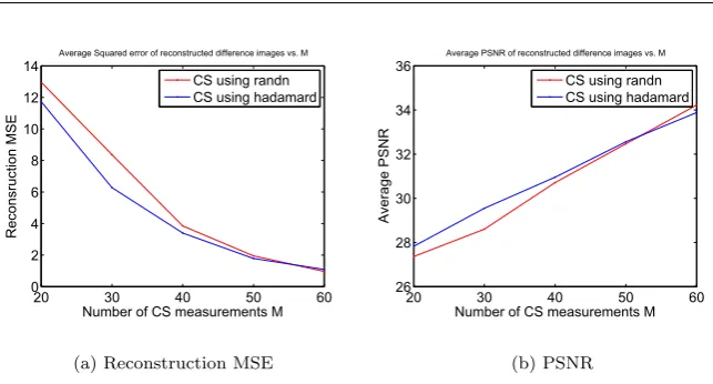
Fig. 12 Comparing reconstruction MSE and PSNR using randn and walsh sensing matrices for ”Shopping center 2” with K=11%

achieved with lowerM, reduced to 50 and 60 for Shopping center ”1” and ”2” respectively compared to multi-target tracking while maintaining least MSE and 33dB PSNR. As a result, making CS adaptive helps in increasing the compression rate and also avoiding the waste of using a higher value ofM at the times where the image is sparse allowing for lowerM. The above discussion reflects the reduction in channel bandwidth using CS by 72%, where instead of transmitting the whole (256×256) image, the compressed measurements of size (70×256) are transmitted. Whereas for more sparse images the reduction reaches 82% of the total image size.

CS states that when enough measurements are used for compression, the reconstruction is done with high accuracy depending on a lower bound ofM. Trajectory tracking of moving targets is considered to reflect the degree of reconstruction accuracy and how accurate the target is detected. For differ-ent datasets according to sparsity levels, M is dynamically chosen based on adaptive CS, Fig.13 shows the (x,y) position plots of the path tracked for the targets in the camera’s scene after CS reconstruction. It illustrates how the trajectory of the tracked targets after the CS reconstruction matches those of the real frame before compression.

Fig.14 shows trajectory tracking for multi targets for dataset”4” ”Walking” after undergoing the different phases; detection, CS and reconstruction.

0 50 100 150 200 250 0

50 100 150 200 250

X coordinates

Y coordinates

Trajectory of tracked targets for M=90

target 1 real trajectory target 1 trajectory after reconstruction target 2 real trajectory target 2 trajectory after reconstruction

(a) Walking men dataset, M=90

60 80 100 120 140 160 180 200 220 240 0

50 100 150 200 250

X coordinates

Y coordinates

Trajectory of tracked target for M=50

target real trajectory target trajectory after reconstruction

(b) Shopping center 1, M=50

60 80 100 120 140 160 180 60

80

100

120

140

160

180

200

220

240

260

X coordinates

Y coordintaes

Tajectory of tracked target for M=60

target real trajectory target trajectory after reconstruction

(c) Shopping center 2, M=60

Fig. 13 Comparing trajectory of detected targets after CS reconstruction for 3 different datasets

the main objective to save sensor nodes power and as a result maximizes their lifetime.

After choosing appropriate compression rates for different sparse datasets, the probability of detection Pdcs after CS and image reconstruction is

ana-lyzed to study the impact of adaptive CS on the performance of the detection problem. Fig.15 shows Pdcs for ”Waking men” dataset with respect to

(a) detected targets (b) only human detected targets

(c) Background subtracted frame elimi-nating vehicles

(d) Predicted trajectory tracking for multi-targets

Fig. 14 Comparing trajectory tracking of moving targets for dataset ”4” (Walking)

and as a result lowPdcs. On the other hand, asM increases thePdcs increases

till nearly reaching≈100% and a 35dB PSNR.

Fig.16 shows thePdcs using CS for different sizes of sensing measurement

matrices and different sparsity levels. As shown, for more sparse images (Less K)the probability of detection reaches≈100% requiring lower values ofM. For instance, an image withK= 3% means that the number of nonzero elements are only 3% of the total size of the image and the remaining 97% are zeros. This is an indication that either few number of targets are present or the camera is zoomed out so the targets’ size is small compared to the total scene. For an images withK= 3% thePdcs reaches≈100% withM = 40. Whereas,

10 20 30 40 50 60 70 0.4

0.5 0.6 0.7 0.8 0.9 1

M

Pdcs

(a)

0 5 10 15 20 25 30 35 0.4

0.5 0.6 0.7 0.8 0.9 1

PSNR

Pdcs

M=20

M=70

M=30

M=50

M=40

M=60

(b)

Fig. 15 Probability of detecting a target after CS reconstruction vs. (a) M and (b) recon-struction PSNR for ”Walking men” dataset

will be a waste for a 97% sparse image to be compressed by projecting a sensing measurement matrix withM = 70 at the time it could be compressed with a sensing measurement matrix withM = 40 without compromising the detection probability. Furthermore, if lower values of M are used with less sparse images, CS fails to achieve a high PSNR of reconstructed images, and as a result the probability of detection is affected.

10 20 30 40 50 60 70 80 90 0

0.1 0.2 0.3 0.4 0.5 0.6 0.7 0.8 0.9 1

M

Pdcs

K=3% K=11% K=20% K=30%

Fig. 16 Probability of detection using CS vs. M for different percentage of sparsity levels

6.4 Analysis of the Probability of missed detection for CS-based duty-cycled WVSN

choosing wrong values ofM as shown in Fig.17. As previously mentioned, the values ofM should be dynamically altered according to the sparsity nature of images. For illustration, Fig.17(a) and 17(b) consider different levels of sparse imagesK= 30% and 11%, respectively. If values ofM are lower than required, the compressed image cannot be reconstructed properly, hence the probability of missing a given target increases compared to previous analysis without the integration of CS. To maintain the same probability of detection as without in-corporating CS to the detection problem, CS adaptively chooses the optimum values of M according to sparsity levels. For instance, Fig.17(a) shows that for aK= 30% image, 70 measurements are required to achieve the samePmd, while to achieve the same performance of detection for a more sparse image (K= 11%) without wasting energy of the communication channel bandwidth, Fig.17(b) shows thatM is reduced to 40 measurements. If the value of M is kept constant regardless of the sparsity nature of different images two cases might occur; (i) if the value of M is lower than required, the probability of missed detection increases due to low PSNR reconstructed images, as a re-sult affecting the performance of the detection problem, or (ii) if the value of

M is higher than required, more measurements are produced whereas more compression could be applied, hence wasting communication bandwidth.

Results prove that selecting duty cycles and dynamically choosing the ap-propriate compression rates for different images and videos according to their sparsity nature, the same performance of detection is achieved as in [8] (be-fore integrating adaptive CS). In addition reducing the size of transmitted data that saves more energy which is one of the main constraints in WVSNs. Hence, adaptive CS is capable of reaching the maximum compression rate per dataset without compromising the probability of detection.

0.2 0.3 0.4 0.5 0.6 0.7 0.8 0.9 1 0

0.1 0.2 0.3 0.4 0.5 0.6 0.7

Bs

Pmd

no CS K=30%, M=20 K=30%, M=50 K=30%, M=70

(a)

0.2 0.3 0.4 0.5 0.6 0.7 0.8 0.9 1 0

0.1 0.2 0.3 0.4 0.5 0.6 0.7 0.8

Bs

Pmd

No CS K=11%, M=10 K=11%, M=30 K=11%, M=40

(b)

Previous results presented so far refer to the cases where a single target enters the monitored area. However, analyzing the impact of multi-targets entering the monitoring area at the same time on the probability of missed detection is challenging. Analysis are carried out on the CS-integrated target detection scenario to evaluate the impact of multi-targets on the probability of missed detection, where CS adaptively chooses the value ofM based on the new sparsity level of the image, as the presence of multi targets, the number of non-zero elements in the background subtracted image is expected to increase. The K and M analysis are then carried out to illustrate the impact of changing the number of targets on the probability of missed detection. It is assumed that a single sensor can detect and take a snapshot of multiple targets crossing its sensing area. Fig.18 shows the effect of various number of targets entering the sensing area at the same time in the CS scenario for a given sparsity level image and adaptively chosing value of CS measurementsM. The targets enter with a velocityv= 15m/s,rsis set to 50, N = 50 sensor nodes are deployed andts is set to 50sec. Fig.18(a) shows the probability of missing all incoming targets (2,4 and 6) as a function ofβs, by increasing the number of incoming targets the probability of missing all targets becomes lower than Pmd of a single-target (solid line). While in Fig.18(b),Pmois shown as a function ofβs for various number of incoming targets (2,4 and 6), it is clear that by increasing the number of monitored targets, there is a probability that at least one of the targets is not detected.

0.1 0.2 0.3 0.4 0.5 0.6 0.7 0.8 0.9 1 0

0.05 0.1 0.15 0.2 0.25

Bs

Pma

K=30%, M=70, Nt=1 K=30%, M=70, Nt=2 K=30%, M=70, Nt=4 K=30%, M=70, Nt=6

(a)

0.1 0.2 0.3 0.4 0.5 0.6 0.7 0.8 0.9 1 0

0.1 0.2 0.3 0.4 0.5 0.6 0.7 0.8

Bs

Pmo

K=30%, M=70, Nt=2 K=30%, M=70, Nt=4 K=30%, M=70, Nt=6

(b)

6.5 Energy complexity

To illustrate the energy saving after applying CS, we used the energy model in [35], where energy cost dissipated by a node over a distancedis denoted by

Etx as shown in (19).

Etx=Eelec∗k+eamp∗k∗d2 (19)

Where,kis size of compressed data (samples) transmitted,Eelec= 50nJ/bit, is the energy being used to run transmitter and receiver circuit, eamp = 100pJ/bitfor the transmitted amplifier.

Table 1 Transmission energy using CS, block CS and without CS for different k

Dataset with/without CS Size of transmitted data k Transmission Energy Etx

without CS

”Walking men” 64K 3.3mJ

”Shopping center 1” 64K 3.3mJ

”Shopping center 2” 64K 3.3mJ

CS

”Walking men” 17K 0.85mJ

”Shopping center 1” 15K 0.7mJ

”Shopping center 2” 12K 0.6mJ

In WVSNs, most energy dissipated is during the transmission and recep-tion, in our case the reception is the base station node which is assumed not to be battery-powered. Hence minimizing transmission energy can have more impact on energy saving [36, 37] Assuming all sensor nodes have the same unit distancedfrom the receiver side, Table.1 shows the energy dissipated during transmission for different k (number of data samples transmitted). As illus-trated, according to different k (which varies depending on compression rates due to sparsity levels), there is an average of≈70% energy saving as compared to transmitting the captured image without CS.

Table 2 Adaptive CS computational time for 3 datasets

Dataset Computational time

”Walking man” 0.03s

”Shopping center1” 0.005s

”Shopping center2” 0.0055s

7 Conclusion

The performance of target detection in WVSNs may degrade due to many factors such as node deployment, number of nodes, velocity and position of targets. Moreover, by integrating CS with the detection problem, the perfor-mance may degrade more than the desired and acceptable level. This is due to other factors such as image sparsity and, loss of information in compres-sion. Hence, there is always a tradeoff between energy consumption (network lifetime) and detection performance. As a result, we derived the first analyt-ical framework for the target detection problem, where the performance is tested in terms of the probability of missing a target. Experiments were tested on comprehensive standard datasets with different sparsity levels resembling indoor and outdoor scenes for single and multiple targets detection. Differ-ent sparsity levels were examined to investigate the effect of sparsity on the chosen compression rates. As a result of this framework, analysis revealed a very interesting result, that by selecting duty cycles and dynamically choosing the appropriate compression rates for different images and videos according to their sparsity nature, the desired performance of detection can be achieved with adaptive CS and at the same time saving energy. Adaptive CS is therefore a strong candidate where on average energy waste is reduced by approximately 70% as compared to transmitting the captured image without CS.

References

1. F.G.H.Yap and H.H.Yen, “A survey on sensor coverage and visual data captur-ing/processing/transmission in wireless visual sensor networks,”Sensors, vol. 14, pp. 3506–3527, February 2014.

2. T.Winkler and B.Rinner, “Security and privacy protection in visual sensor networks: A survey,”ACM Computing Surveys (CSUR), vol. 47, no. 1, July 2014.

3. F.Wang and J. Liu, “Networked wireless sensor data collection:issues, challenges, and approaches,”Communications Surveys and Tutorials, IEEE, vol. 99, pp. 1–15, 2010. 4. S.Soro and W.Heinzelman, “A survey on visual sensor networks,”Hindawi publishing

corporation, Advances in Multimedia, vol. 2009, no. 640386, pp. 1–21, May 2009. 5. Y.Charfi, B.Canada, N.Wakamiya, and M.Murata, “Challenges issues in visual sensor

networks,” inIEEE on wireless Communications, April 2009, pp. 44–49.

6. I.F.Akyildiz, T.Melodia, and K.R.Chowdhury, “A survey on wireless multimedia sensor networks,”computer Networks, vol. 51, pp. 921–960, March 2007.

7. Q.Cao, T.Yan, J.Stankovic, and T.Abdelzaher, “Analysis of target detection perfor-mance for wireless sensor networks,” inIn DCOSS05, 2005, pp. 276–292.

8. P.Medagliani, J.Leguay, G.Ferrari, V.Gay, and M.Lopez-Ramos, “Energy-efficient mo-bile target detection in wireless sensor networks with random node deployment and partial coverage,”Pervasive and Mobile Computing, vol. 8, no. 3, p. 429447, 2012. 9. Y.Wang and D.Wang, “Energy-efficient node selection for target tracking in wireless

sensor networks,”International Journal of Distributed Sensor Networks, vol. 2013, 2013. 10. O.Demigha, W.K.Hidouci, and T.Ahmed, “On energy efficiency in collaborative target tracking in wireless sensor network: A review,”IEEE Communications Surveys Tuto-rials, vol. 15, no. 3, 2013.

12. E.J.Candes and M.B.Wakin, “An introduction to compressive sampling,”IEEE Signal Processing Magazine, pp. 21–30, March 2008.

13. D. Donoho, “Compressed sensing,”IEEE Transactions on Information Theory, vol. 52, no. 4, pp. 1289–1306, 2006.

14. M.Zhao, A.Wang, B.Zeng, L.Liu, and H.Bai, “Depth coding based on compressed sens-ing with optimized measurement and quantization,”Ubiquitous International Journal of Information Hiding and Multimedia Signal Processing, vol. 5, no. 3, pp. 475–484, July 2014.

15. C.Patsakis and N.G.Aroukatos, “Lsb and dct steganographic detection using compres-sive sensing,”Ubiquitous International Journal of Information Hiding and Multimedia Signal Processing, vol. 5, no. 4, pp. 20–32, January 2014.

16. V.Cevher, A.Sankaranarayanan, M. Duarte, D.Reddy, R. Baraniuk, and R.Chellappa, “Compressive sensing for background subtraction,” 2008.

17. A.Mahalanobis and R.Muise, “Object specific image reconstruction using a compressive sensing architecture for application in surveillance systems,” IEEE Transactions on Aerospace and Electronic Systems, vol. 45, no. 3, pp. 1167–1180, July 2009.

18. C.T.Chou, R.Rana, and W.Hu, “Energy efficient information collection in wireless sen-sor networks using adaptive compressive sensing,” inIEEE 34th Conference on Local Computer Networks (LCN), Zrich, Switzerland, October 2009, pp. 443–450.

19. E.J.Candes and B.Recht, “Exact matrix completion via convex optimization,”CoRR, vol. abs/0805.4471, 2008.

20. S.Fayed, S.M.Youssef, A.El-Helw, M.Patwary, and M.Moniri, “Adaptive compressive sensing for target tracking within wireless visual sensor networks-based surveillance applications,”Multimedia Tools and Applications, vol. 75, no. 11, pp. 6347–6371, 2016. 21. R. Baraniuk, “Compressive sensing,”IEEE Signal Processing Magazine, pp. 118–124,

July 2007.

22. E. Wang, J. Silva, and L. Carin, “Compressive particle filtering for target tracking,” in

IEEE/SP 15th Workshop on Statistical Signal Processing, SSP, September 2009, pp. 233 –236.

23. J.Romberg, “Imaging via compressive sampling,”IEEE Signal Processing Magazine, pp. 14–20, March 2008.

24. H. C. Huang and F. C. Chang, “Robust image watermarking based on compressed sensing techniques,”Journal of Information Hiding and Multimedia Signal Processing, vol. 5, no. 2, pp. 275–285, April 2014.

25. E.J.Candes, “Compressive sampling,” inProc. of the International Congress of Math-ematicians, 2006.

26. A.Hormati, O.Roy, Y.M.Lu, and M.Vetterli, “Distributed sampling of signals linked by sparse filtering: theory and applications,”IEEE Transactions on Signal Processing, vol. 58, no. 3, pp. 1095–1109, March 2010.

27. J. Tropp and A. Gilbert, “Signal recovery from random measurements via orthogonal matching pursuit,”IEEE Transactions on Information Theory, vol. 53, no. 12, pp. 4655–4666, December 2007.

28. P.Medagliani, J.Leguay, V.Gay, M.Lopez-Ramos, and G.Ferrari, “Engineering energy-efficient target detection applications in wireless sensor networks,” inIEEE Interna-tional Conference on Pervasive Computing and Communications (PerCom), March 2010, pp. 31–39.

29. Z.Wang, G.R.Arce, B.M.Sadler, J.L.Paredes, and X. Ma, “Compressed detection for pi-lot assisted ultra-wideband impulse radio,” inIEEE International Conference on Ultra-Wideband ICUWB, September 2007, pp. 393–398.

30. M.A.Davenport, M.B.Wakin, and R.G.Baraniuk, “Detection and estimation with com-pressive measurements,” Rice University, Department of ECE, Technical Report, Tech. Rep., 2006.

31. F. Cheng and Y. Chen, “Real time multiple objects tracking and identification based on discrete wavelet transform,”Elsevier Pattern Recognition Journal, vol. 39, p. 1126 1139, 2006.

32. “Caviar datasets,” Dataset: EC Funded CAVIAR project/IST 2001 37540, http://homepages.inf.ed.ac.uk/rbf/CAVIAR/, 2001.

34. H. Jiang, W. Deng, and Z. Shen, “Surveillance video processing using compressive sens-ing,”arXiv preprint arXiv:1302.1942, 2013.

35. Ms.V.MuthuLakshmi, “Advanced leach protocol in large scale wireless sensor networks,”

International Journal of Scientific and Engineering Research, vol. 4, no. 5, pp. 248–254, May 2013.

36. A.Redondi, D.Buranapanichkit, M.Cesana, M.Tagliasacchi, and Y.Andreopoulos, “En-ergy consumption of visual sensor networks: Impact of spatio-temporal coverage,”IEEE tranaction on Circuits and Systems for Video Technology, vol. 24, no. 12, pp. 2117–2131, December 2014.