R E S E A R C H
Open Access
A novel jammer detection framework for
cluster-based wireless sensor networks
P. Ganeshkumar
*†, K. P. Vijayakumar
†and M. Anandaraj
Abstract
Jamming attack is a serious security threat in wireless sensor networks. Therefore, it is important to frame a mechanism to protect wireless sensor networks from various jamming attacks. Jammer intrusion detection and jamming detection are two separate issues. In this paper, a novel jammer detection framework to detect the intrusion of jammer and the presence of jamming in a cluster-based wireless sensor network is proposed. The proposed framework is novel in three aspects: whenever the cluster head receives a packet, it first verifies whether the source node is a legitimate, new node, or a jammer node. Second, when the source node is declared as a new one in the first step, then the framework validates whether the new node is legitimate node in the previous cluster or a jammer node by using cluster head code. Third, the framework observes the behavior of the newly joined node and the existing nodes to identify whether the nodes in the cluster is jammed or not. Additionally, it also classifies the types of jamming, if the presence of jamming is detected. Simulation result shows that the proposed framework performs extremely well and achieves jamming detection rate as high as 99.88 %.
Keywords: Wireless sensor networks, Threat, Jammer, Jamming, Cluster
1 Introduction
Wireless sensor network encompasses small sensor nodes. The sensor node includes sensing unit, computing unit, communicating components, and memory [1]. Sensor nodes are self-organized. These nodes are deployed in a region called sensor field to sense the environment. Sen-sor nodes are restricted by memory space, energy, and computational power. The sensor nodes work in an infras-tructureless and dynamically changing environment [2] and route the collected data to the destination node for further interpretation.
Clustering results in a two-layer hierarchy where the cluster heads (CHs) form the higher layer and cluster members form the lower layer. Nodes are divided into clusters in the cluster-based wireless sensor networks. Each cluster contains a CH and cluster members (CMs). In a cluster, communication among CMs is carried out through CH and communication among CHs is carried out through the base station (BS). The CM may leave from a cluster and join in another cluster, and a new node may
*Correspondence: [email protected] †Equal contributors
Department of Information Technology, PSNA College of Engineering and Technology, Kothandaraman Nagar, Dindigull, Tamil Nadu 624622, India
join in a cluster. The benefits of clustering are achiev-ing energy efficiency by reclusterachiev-ing, decreasachiev-ing colli-sion, reducing the communication overhead, improving throughput, and network lifetime [3].
The sensor network is vulnerable to jamming attacks since the sensor nodes operate at a very low radio power [4] and use limited communication range between source and sink. The jammers initiate jamming attacks, and their objective is to prevent the communication between sensor nodes or corrupt legitimate transmissions of sensor nodes by causing intentional packet collisions at the medium. Therefore, wireless sensor networks are appropriate in their hunt for jammers. The sensor networks are enor-mously used in many applications from military to health care [1, 3, 5, 6]. Therefore, a mechanism is required to detect jammer intrusion and jamming in wireless sensor network (WSN). To detect jammer intrusion and jam-ming, first, the intrusion or entry of jammer has to be detected (by using verification and validation algorithm) then, jamming and its types are detected (by using audit-ing algorithm). In this paper, a novel jammer detection framework (which detects the intrusion of jammer and various types of jamming attacks) is proposed and eval-uated. In the existing literature [7–10], various jamming
detection approaches are proposed for detecting jamming in the wireless sensor networks. However, to the best of our knowledge, none of the existing literature has con-sidered the issue of jammer intrusion detection in sensor networks. Therefore, in this paper, the main idea is both jammer intrusion detection and jamming detection in the cluster-based wireless sensor networks. throughout this paper, jammer detection refers to (i) jammer intrusion detection and (ii) jamming detection.
To understand jammer intrusion detection, it is assumed that a legitimate member moves from one cluster to another cluster. At this juncture, the jammer imperson-ates as a legitimate member and enters into a new cluster posing to be as legitimate member. For example, when a member M1 moves from cluster C1 to cluster C2, then according to existing reassociation procedure, C2 has to validate with C1, whether M1 is a legitimate member in C1 or not. If C2 receives a reply from C1 stating that M1 is a legitimate node in C1, then C2 ascertains that M1 is a legitimate member. At this point of time, the jam-mer node poses to be M1 enters into the cluster C3. In order to check the legitimateness of M1, C3 queries C1 and obviously receives a reply that M1 is a legitimate node in C1. By posing to be a moving legitimate node, jam-mer node cleverly enters into C3. This problem has to be addressed. To alleviate this problem, in this paper, the idea of cluster head code (CHC) is deployed and it is described in Section 3.1.1. The jammer node is also referred as rouge node within the WSN. The reason to consider the rouge/jammer node in the WSN is given as follows: when a member M1 moves from cluster C1 to cluster C2, the jammer node posing to be M1 enters into the cluster C3. After entering into C3, the jammer node can jam the members of C3 that are within the communication range of the jammer node.
To understand jamming detection in cluster-based WSN, let a cluster with cluster head and cluster mem-bers be considered. In order to detect the presence of jamming in the network (to detect whether the cluster members are jammed or not), a mechanism is needed to monitor the behavior of the cluster members peri-odically. To address this, auditing algorithm is devised (Section 3.1.2). In the auditing algorithm, the behavior of the members are determined periodically by using two jamming detection metrics such as packet delivery ratio (PDR) and received signal strength indicator (RSSI). Auditing algorithm is implemented in CH. This algorithm computes the PDR, maximum PDR, and malicious level of CMs in the cluster periodically (say for every 0.1, 1, and 3 s, respectively). PDR alone is inadequate in deter-mining the presence of jamming. Therefore, RSSI is used as an additional metric to detect the presence of jamming accurately. When the maximum PDR of a CM is lower than the PDR threshold (Section 2.5.2), then auditing
algorithm measures the RSSI of the corresponding CM. The measured RSSI is compared with the RSSI thresh-old (Section 2.5.2). If the measured RSSI is above the RSSI threshold value, then auditing algorithm assigns the malicious level as high. If the malicious level of the corre-sponding CM is thrice consecutively determined as high, then the auditing algorithm declares that the correspond-ing CM is jammed. The type of jammcorrespond-ing is also identified if the presence of jamming is detected in the auditing algorithm.
The primary motivation of this novel jammer detection framework is to identify the intrusion of the jammer and the jamming attacks in the cluster. The key ideas of this framework are listed below:
• The proposed framework uses CH centric (network centric) approach for detecting jamming in the cluster-based sensor network. In this approach, the CH estimates the metrics PDR and RSSI to make decision about “jammed situation” or “non-jammed situation”. The metrics PDR and RSSI for each node under a single cluster is implicitly known to the CH, and it is explicitly not necessary for the CH to collect metrics from the CMs. Due to this, processing and decision-making are carried out by the CH itself without help from the members unlike the existing system. In the existing system, packet send ratio (PSR), PDR, bad packet ratio (BPR), and bit error rate (BER) are termed as jamming induction metrics (JIM), and they are gathered from respective nodes as well as neighbor nodes and are based on the collected JIM where the decision on the presence of jamming is determined. In the proposed system, the identified JIM metrics are PDR and RSSI. PDR and RSSI of CMs are available within the CH itself, and it is not required to collect this metrics elsewhere from the CMs. Therefore, it can be claimed that the CM is not burdened (is not loaded heavily) in the proposed approach.
• As discussed above, in the proposed system, the communication overhead is reduced since CH by itself directly estimates the metrics for processing and decision-making (CH does not depend on its
member for collecting the JIM), the communication overhead is reduced.
• In the proposed work, a new node may join in a cluster or an existing node may leave from a cluster. Therefore, it supports mobility unlike the existing system which does not support mobility. To support this, the modified medium access control (MAC) frame format is used. The modified frame format also authenticates the newly joining node in the cluster (Section 3.1.1).
• Jamming detection metrics (Section 2.3): Jamming detection level is bounded by threshold values of PDR and RSSI. That is, if PDR decreases below a given threshold value and RSSI is higher than its threshold value, then it can be ascertained that the jamming is present. Predicting this PDR and RSSI threshold is a crucial task in WSN. In this paper, appropriate statistical test (T test) is carried out to find and fix the threshold values.
• Statistical proof (Section 2.5): By using PDR and RSSI threshold, the presence of jamming can be
determined. However, it is not sufficient to determine the presence of jamming alone, further it is necessary to determine the type of jamming launched (constant or deceptive or random or reactive jamming). In order to find the type of jamming launched in the network,T test is performed on the two sets viz PDR is not affected without jamming and PDR is affected after launching specific type of jamming. TheT test proves that there is a significant difference between the two means. By using the mean PDR of a jammed member as reference value, the classification of jamming is performed (Table 1). In addition to this, chi-square test is performed to compare the performance of the anticipated result and the result obtained from simulation (Table 11).
• Jammer detection framework (Section 3): The jammer detection framework (JDF) detects the intrusion of the jammer and various types of jamming attacks. This framework works in three aspects. First, it performs verification whenever a packet is received. Next, whenever a node joins in a cluster then the framework uses cluster head code (CHC) in order to determine the presence of jammer (whether the node wishes to join in a cluster that is legitimate node or jammer node). Finally, the
framework monitors the behavior of both the existing node and the newly joined node periodically to determine the presence of jamming.
• Authentication using CHC (Section 3.1.1): The proposed framework uses CHC to determine whether the new node belongs to the available cluster. Because the jammer node finds the loop hole and enters into the cluster during node mobility, that is, the jammer node may pose as a legitimate member
Table 1Types of jamming
Types of jammer Average PDR (in %) PDR range (in %) RSSI (in db)
Constant 9.76 0–10 −93.141
Deceptive 28.81 25.6–53.5 −93.141
Random 57.9 53.6–73.75 −93.141
Reactive 22.21 11–25.5 −93.141
of other clusters and cleverly enter into the cluster as a legitimate node.
The rest of the paper is organized as follows: The sys-tem model is described in Section 2. Section 3 explains the proposed framework in three aspects: verification, validation, and auditing. Experiments and discussions on the results are presented in Section 4. Related work is discussed in Section 5. Finally, Section 6 concludes this paper.
2 System model
In this section, different types of jamming attack mod-els are discussed first, and then the metrics used in the existing system are discussed. Next, the metrics used for detecting the presence of jamming in the proposed work is described. Finally, the system configuration is depicted for determining the effect of various types of jamming.
2.1 Jamming attack models
The proposed work employs four types of jamming mod-els, namely constant, deceptive, random, and reactive jammers [7]. The constant jammers continuously gener-ate packets on the medium to jam the communication completely and do not obey the procedures of the MAC layer. The deceptive jammer regularly provides packets (not random bits) on the communication channel. It is a dangerous type of jammer since deceptive jammer follows the MAC layer procedure. The random jammer produces the packets in a regular interval and switches between jamming and sleeping. This type of jammer sleeps for a period ofRStime and jams for a period ofRJ time. The
RS and RJ values may either be fixed or be in random. As a result, the random jammer can reduce the power consumption by switching between sleep and jam modes. During jam period, the random jammer may operate as constant or deceptive jammer. The reactive jammer listens to the communication channel and generates fake packet when transmission happens.
node to the total number of packets arrived at destina-tion node. The SNR is defined as the ratio of the received signal power in a node to the received noise power in a node. The ECA is defined as the amount of energy con-sumed in a particular time for a wireless sensor network. The BER is computed as the ratio of the number of dam-aged bits to the number of total bits received by a node for the duration of a transmission session.
The metrics PSR and PDR are used in [7] to identify the jamming attack. From the results, it is observed that the PSR and PDR encounter problems in deciding about jamming and its types. Then, two algorithms are devised (signal strength consistency check and location consis-tency check). The first algorithm uses the PDR and signal strength in order to determine the presence of jamming. The second algorithm uses the PDR and location of its neighbors to determine the presence of jamming. The estimation of PSR is a complex task. Additionally, this approach needs localization technique or hardware such as GPS to identify the neighbor’s location. The BPR and the SNR metrics are used in [8] to detect various jamming attacks. The approach used in [8] causes communication overhead since every node in the network has to report the data periodically to the BS. The metrics PDR, BPR, and ECA are used in [9] to detect the presence of jamming. The BPR and ECA are estimated by nodes; accordingly, the nodes are burdened. The metrics BER and RSS are used in [10] for detecting jamming attacks. But it is diffi-cult to compute the BER by a sensor node, since a sensor node needs to collect a huge amount of data. This method cannot classify various types of jamming attacks. It is clear from the existing jamming detection metrics that there is no metric or combination of metrics that determines jam-ming and its types in both physical and data link layer. Therefore, a kind of jamming detection metric and its suitability in WSN are needed to be explored.
2.3 Jamming detection metrics in the proposed system In the proposed system, the jamming detection metrics, namely PDR and RSSI, are selected for detecting the pres-ence of jamming in a wireless sensor network. The PDR alone is not sufficient to detect the presence of jam-ming. Therefore, it is essential to consider an additional metric to detect the presence of jamming and different types of jamming correctly. The metric RSSI is consid-ered as an additional metric as discussed in Section 2.2. The advantages of selecting these metrics are discussed as follows:
1. The PDR is an excellent metric since the CH can measure it by itself accurately without much computational overhead, and PDR can identify the presence of all types of jamming attacks both at physical and data link layers.
2. The CH can easily measure RSSI either by using formulae as per the chosen propagation model (in the proposed work, free-space propagation model is chosen) or by the node’s RF power meter.
3. In the proposed system (Section 3), the CH estimates the metrics (PDR, RSSI) and makes decision about “jammed situation” or “non-jammed situation”. The metrics PDR and RSSI for each node under a single cluster is known to the CH implicitly, and it is explicitly not needed for the CH to collect the metrics from the nodes. Due to this, processing and decision-making are done by the CH itself without needing help from the members. Therefore, it can be claimed that the CM is not burdened (is not loaded heavily). 4. In the proposed system, the metrics PDR and RSSI
are used in detecting the presence of jamming and its types to an extend of 99.9 %. The metrics PDR and RSSI are defined in the next section. The suitability of considering these metrics in the WSN
environment is illustrated in Section 2.5.
2.4 Description of PDR and RSSI
This section describes the metrics that are used in this paper to detect the presence of jamming attack. The met-rics PDR and RSSI are considered in the proposed system. The PDR is computed by a source node (CH). The PDR is defined as the ratio of the total number of packets success-fully (the packets for which acknowledgement is received) sent by the node to the total number of packets sent by the node. The PDR is expressed as follows:
PDR=Pss/Ps (1)
where Pss is number of packets successfully sent by the source, Ps is the total number of packets sent at the source. The RSSI is defined as the ratio of received signal strength to the reference power. The received signal strength value can be converted into RSSI [11] as given below:
RPr=TPs.Gt.Gr
where RPr is the remaining power at the receiver, TPs is the transmitted power at the sender, Gt is the gain of the transmitter, Gr is the gain of the receiver,βis wave length,
dis distance between the sender and receiver, and Pref is the reference power.
2.5 Statistical proof
significant difference between the two population means (i.e., observed PDR during jamming-free scenario and observed PDR after the launching of jamming). By using the mean of samples, the PDR threshold is fixed. Lastly, by using PDR and RSSI threshold, the presence of jamming is determined. However, it is not sufficient to determine the presence of jamming alone, but further it is neces-sary to determine the type of jamming launched (constant or deceptive or random or reactive jamming). In order to find the type of jamming launched in the network,T test is performed on the two sets viz observed PDR during jamming-free scenario and observed PDR after launching a specific type of jamming. TheT test proves that there is a significant difference between the two means. There-fore, by using the mean PDR of the jammed member as reference value, the types of jamming are classified (all the
Ttests are performed by using samples obtained from our simulation).
2.5.1 Jamming and PDR
The T test is performed to verify whether the jamming infuences PDR or not by using few samples. The simu-lation is carried out in Section 4. At first, the constant jamming is commenced. Then, two group of samples are taken from the simulation with respect to the absence and presence of jamming in the sensor network. TheTtest is done on these samples to signify whether there is a vari-ation between the two populvari-ation means (that is, PDR is not affected during the absence and presence of jamming) or not. Similarly, the simulation is repeated for other types of jamming.
The null hypothesis signifies that there is no differ-ence between the two population means (i.e., PDR is not affected during the absence and presence of jamming). The alternate hypothesis signifies that there is a differ-ence between the two population means (i.e., PDR is not affected in the absence of jamming and PDR is affected in the presence of jamming).
Ttest is done on 40 samples (20 samples in the absence of jamming and 20 samples in the presence of jamming) of PDR acquired from the CMs, CM1, CM2, CM3, CM4, and CM5. The degree of freedom (df) is computed as 38 (s1+s2−2), and the significance level (p) is 0.001 with the correspondingtvalues 49.2, 68.7, 72.2, 0.6, and 2.1 for 99.9 % of confidence interval.s1 indicates the total num-ber of samples measured in the absence of jamming, and
s2 denotes the total number of samples in the presence of constant jamming. The result passes thettest. Thetvalue of members CM1, CM2, CM3, CM4, and CM5 is 49.2, 68.7, 72.2, 0.6, and 2.1, respectively. Thettable value of
T test is 3.65. It is identified that thetvalue of the CMs, CM1, CM2, and CM3, exceeds the table value. This sig-nifies that the PDR of CM1, CM2, and CM3 is reduced due to jamming, whereas the members CM4 and CM5
are not affected by constant jamming. Thus, it proves the significance of alternate hypothesis for constant jamming. The level of significance is 0.001. This indicates that the reliability of the result is 99.9 %, i.e., the obtained result is considered to be correct by 99.9 % and the chance of attained result to be wrong is 0.1 %. Similarly, theT test is repeated for other types of jamming (deceptive, random, and reactive).
2.5.2 PDR and RSSI threshold
PDR is employed to realize the incidence of jamming. Therefore, it is necessary to identify the association between PDR and jamming. It is well known that jamming is inversely proportionate to PDR. An analysis is done to find out the snapping point at which the jammer influ-ences the PDR to decrease. In the proposed system, the snapping point at which the jammer influences the PDR to diminish is fixed as the threshold value (in simulation) to forecast the presence of jamming.
CH periodically monitors the PDR. If the computed PDR is lesser than the PDR threshold, then CH will state that jamming has taken place. The test is done with four samples of PDR acquired from CMs CM1, CM2, CM3, CM4, and CM5 to fix the threshold. The degree of free-dom is 3, and the significance level (p) is 0.001 with the corresponding t value at 13.1 for 99.9 % of confidence interval. The result passes thettest. Thettable value ofT
test is 12.92. It is identified that thetvalue (13.1) exceeds thettable value (12.92). This shows that there is signifi-cance and therefore the PDR threshold (PDR threshold) is fixed as 74.75.
The factors other than jamming such as collision and congestion can also influence the data transmission and cause the PDR value to become low. Therefore, PDR is used in conjunction with RSSI in order to detect the presence of jamming. The CH frequently measures the RSSI value and fixes the RSSI threshold. If the CH esti-mates lower PDR value than the PDR threshold, then CH also compares an estimated RSSI value against the RSSI threshold. If the observed PDR value is lower than the PDR threshold and the RSSI value is higher than the RSSI threshold, then it can be ascertained that the node is jammed. The average RSSI (db) threshold (RSSI threshold) value is fixed as−93.141 for 20 m [12].
2.5.3 Types of jamming
The CH compares the observed PDR and RSSI against the PDR range and RSSI as shown in the Table 1 to make a distinction between various types of jamming. Table 1 consists of three fields such as average PDR, PDR range, and RSSI. The average PDR represents the aver-age PDR value of CMs CM1, CM2, and CM3 from the
as discussed in Section 2.5.1. Similarly, the experiment is repeated for other types of jamming). The PDR range for various types of jamming is considered from the T test (in simulation). For example, in the constant jamming, the PDR range is considered as in Section 2.5.1. Similarly, the experiment is repeated for other types of jamming. The RSSI is fixed as discussed in Section 2.5.2.
2.6 System configuration
The system set-up consists of four clusters and a BS as shown in the Fig. 1. Each cluster consists of six nodes (one CH and five CMs). The communication range of each node in the network is 20 m. CM communicates with other CMs in a cluster through CH and CHs communicate with other CHs through BS. CM moves between clusters. To illustrate the proposed system, a jammer is launched deliberately in the cluster CH21. The proposed system is installed in the CH and BS. To understand the interac-tions of the jamming detection metrics (Section 2.3) and to measure the impact of a jammer in various scenarios (Section 4.2), simulations are performed as per described in Section 4. The simulation is done by using various mod-els as discussed in Section 2.1. In the simulation, a jammer is launched in the first cluster (CH 21). This cluster con-sists of a cluster head (CH21) and five members such as CM1, CM2, CM3, CM4, and CM5. From the simulation result, it is observed that CH21 identifies that the mem-bers CM1, CM2, and CM3 are jammed and the memmem-bers CM4 and CM5 are not jammed. It is also evident from the simulation result that the CH has the ability to make a dis-tinction between various types of jamming (Section 2.5.3). Based on the simulation, it is justified that the CH has the
Fig. 1Wireless sensor network with a jammer node. Thenode in black boxindicates CH, thenodes without boxspecify CMs, and thered node represents the jammer node. Thelineindicates a communication between CH and CM. The arrow denotes communication between CHs and BS. The CH21and members 1 to 5, CH22 and members 6–10, CH23 and members 11–15, and CH24 and members 16–20 are divided into four clusters, respectively. The nodes withcolored box indicate jammed members
ability to identify the jammed members and BS has the ability to identify the jammed CHs.
3 Jammer detection framework
In this section, first, innovation, research idea, and description of the problem statement are described. Next, the modules in the jammer detection framework such as verification and validation (jammer intrusion detec-tion) as well as auditing (jamming detecdetec-tion) are dis-cussed. Then, the databank used in the proposed system is defined. Finally, verification and validation steps as well as auditing step of the jammer detection framework are described.
The important innovation,research idea, and the description of the problem statement of this article are listed in the following. In spite of this, the motivation, objective, and contribution of the paper is well described in Section 1.
1. In the existing literature [7–10], several jamming detection approaches were proposed for flat WSN. In [13], the authors proposed jamming detection approach for cluster-based WSN. Thus, in the existing literature, only jamming detection is carried out. The issue of jamming detection is completely different from jammer detection. Jamming detection refers to the detection of the presence or absence of jamming in the network. Jammer intru-sion detection or simply jammer detection refers to the detection or identification of the entry of jammer node in the cluster. To the best of our knowledge, none of the existing literature has considered the issue of jammer intrusion detection or jammer detection in cluster-based WSN. Therefore, in this paper, the main idea is to first detect the jammer intrusion into the cluster (Section 3.1.1: verification and validation algorithm) and then to per-form jamming detection in the cluster in the cluster-based WSN (Section 3.1.2: auditing algorithm). The proposed system works in two aspects: first, it prevents the entry of jammer into the cluster and, second, it continuously monitors the members inside the cluster to determine whether the members are jammed or not. That is, first, the proposed JDF prevents the entry of the jammer into the cluster. But due to any unexplained or unaddressed random error, if the jammer enters into the cluster then, a monitoring mechanism is needed to monitor the cluster member to determine whether the members are jammed or not. To address this, the cluster head of the proposed system performs jamming detection inside the cluster. Therefore, the proposed JDF comprises two components: verification and validation algorithm for jammer intrusion detection and auditing algorithm for jamming detection within the cluster member.
in existing literatures, in the proposed system, statistical test (Ttest) is performed for the following: (i) To examine and determine the appropriate jamming detection metric (among PDR, PSR, RSSI) for identifying the presence of jamming (Section 2.5.1), (ii) to find the threshold value of PDR (Section 2.5.2), and (iii) to classify various types of jamming (Section 2.5.3).
3. In this paper, a performance metric called unde-tection ratio (UDR) is introduced. To the best of our knowledge, none of the existing literature had defined and used this metric UDR. UDR explains that the CH does not detects a node as abnormal when the node is really jammed (that is, the CH does not detect the jammed node or CH fails to detect a jammed node). The detailed explanation is given below.
The reason behind choosing the metric UDR in this paper is explained as follows: in the existing literature, false positive rate or false discovery ratio or false detec-tion ratio (FDR) was used and defined as the ratio of the number of nodes incorrectly identified by the system to the number of nodes actually falling under that group. There is no clear definition of false detection in the exist-ing literature. In general, there are two scenarios in false detection: (i) detects a node as abnormal though that node is normal (false positive) and (ii) does not detect a node as abnormal when the node is jammed (false negative). It is found from the existing literature that the FDR denotes the first scenario (false positive), and there is no explana-tion about the second scenario (false negative). Therefore, in this paper, the detection of sensor nodes is classified into (i) true detection, (ii) false detection, and (iii) unde-tection. True detection, false detection, and undetection are based on true positive, false positive, and false nega-tive, respectively. In true detection, the CH detects a node as abnormal when the node is jammed. In false detection, the CH faultily detects a node as abnormal though that node is normal. In undetection, the CH does not detects a node as abnormal when the node is really jammed (that is, the CH does not detect the jammed node or CH fails to detect a jammed node) (Section 4.3).
For example, consider there are ten nodes in which five nodes are jammed and five nodes are normal.
• In first scenario, if the jamming detection system detects five nodes as jammed when five nodes are really jammed, then the TDR is computed as 1 (that is,5/5=1). The system neither detects a node as abnormal though that node is normal nor detects a node as normal when the node is jammed. Hence, the FDR and UDR are computed as 0.
• In second scenario, in real scenario, five nodes are jammed out of six nodes. In the simulation, if the system detects six nodes as jammed when only four nodes are really jammed, then the TDR is computed
as 0.8 (that is,4/4+1=0.8). (That is, the number of correctly detected jammed nodes/the number of correctly detected jammed nodes + the number of nodes that are detected as not jammed but they are actually jammed). In this scenario, the FDR is computed as 0.4 (that is,2/(2+3)=0.2). (That is, the number of nodes are detected as jammed but they are normal/the number of nodes that are detected as jammed but they are normal + the number of correctly detected normal nodes, but the nodes are normal). In this scenario, the UDR is computed as 0.2 (that is,1/(4+1)=0.2. That is, the number of nodes that are detected as normal but they are abnormal/ the number of correctly detected jammed nodes + the number of nodes that are detected as normal but they are abnormal).
For a fair jamming detection system, the TDR must be equal to 1 and FDR and UDR must be equal to 0.
3.1 Jammer detection framework model
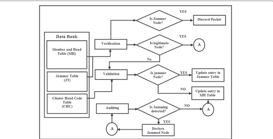
The JDF is proposed for cluster-based wireless sensor networks. The main idea of the JDF is to perform both jammer intrusion detection by using verification and val-idation, and jamming detection using auditing. Figure 2 illustrates the key modules of the framework.
The JDF is implemented in all CH/BS. When this framework receives a packet, then it detects whether the source node is a legitimate node or jammer node or new node using three steps namely: (1) verification, (2) validation, and (3) auditing. Every CH has to maintain look-up tables for verification, validation, and auditing. The look-up tables employed in JDF are cluster mem-ber and head (CMH) table, jammer table, CHC table, cluster member CHC (CM_CHC) table, flag table, PDR table, maximum PDR (MaxPDR) table, and malicious table. All these look up tables are kept inside a data bank.
Fig. 2Jammer detection framework. The framework represents three steps: verification, validation, auditing, and the databank. The databank consists of various look-up tables used by this framework
The description and use of each table is explained as follows:
1. The CMH table contains two fields: Node ID and node type as shown in Table 2. The node ID represents the identity (address) of the nodes. Node type represents the type of the source node (CH, CM, or BS). The objective of this table is to determine the type of the source node.
2. The Jammer table includes two fields such as S.No. and node ID as shown in Table 3. The S.No.
represents the corresponding records’ entry number. The node ID represents the identity (address) of the jammer node. The source node is declared as jammer node, if address of the source node is found in the jammer table.
Table 2CMH table
Node ID Node type
1 M
2 M
3 M
– –
21 H
22 H
– –
50 B
3. The CHC table is formed by two fields namely: cluster heads and CHC as shown in Table 4. The cluster heads field denotes the CHs available in the network. The CHC represents each CH’s CHC (Section 3.1.1). This table is used by each CH to authenticate the source node, when a source node moves from one cluster to the other or when a source node wishes to join in a cluster.
4. The CM_CHC table includes two fields such as cluster head and CHC as shown in Table 5. The cluster head represents the CH in which the corresponding CM has been associated. The CHC denotes the CHC provided by the CH in which the corresponding CM is associated.
5. The flag table contains two fields, namely CM_N and flag, as shown in the Table 6. The CM_N field represents the address of the members in the cluster, and flag represents either the valueT or F, where T denotes a successful delivery of a packet of the corresponding CM andF denotes an unsuccessful (F is determined if there is no acknowledgement within the specified time interval) delivery of a packet. The JDF updates the flag entry with the value eitherT or F in this table.
Table 3Jammer table
S.No. Node ID
Table 4CHC table
Cluster heads CHC
21 5
22 2
23 4
24 6
6. The PDR table consists of two fields such as CM_N and CM_PDR as shown in Table 7. The CM_N field denotes the address of the CM and the CM_PDR field represent the packet delivery ratio of each member in the cluster. The JDF computes this CM_PDR value periodically (every 0.1 s) by observing the entries from Table 6.
7. The MaxPDR table is formed by two fields such as CM_N and CM_MPDR as shown in Table 8. The CM_N field represents the address of the CM, and CM_MPDR represents the maximum packet delivery ratio of each member in the cluster. The JDF
calculates this CM_MPDR value periodically (every 1 s) by observing the entries from Table 7.
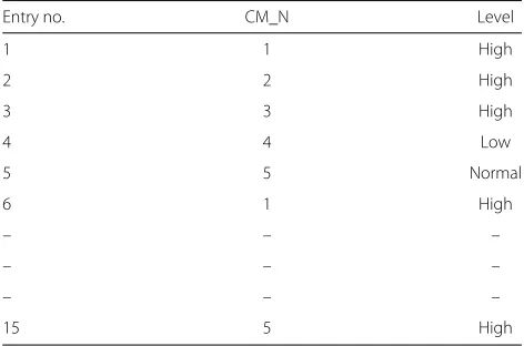
8. The malicious table contains three fields such as entry no., CM_N, and level as shown in Table 9. The entry no. field represents records’ entry number. The CM_N field represents the address of the CM, and level denotes the malicious level of each member in the cluster. The JDF computes the value of Level periodically (every 3 s) by observing the entries from Table 8 and expresses the value as high, normal, and low. In order to do this, the following three rules are followed:
1. If MaxPDR.MPDR is lesser than
PDR_Threshold and RSSI is greater than RSSI_Threshold, then its malicious level is assigned as high.
2. If MaxPDR.MPDR is equal to
PDR_Threshold, then its malicious level is assigned as normal.
3. If MaxPDR.MPDR is greater than
PDR_Threshold, then its malicious level is assigned as low, where MaxPDR.MPDR represents the maximum value of PDR from the corresponding entries of each member in the cluster (every 1 s).
The verification step verifies whether the source node is CM, BS, a new node, or a jammer node by referring the
Table 5CM_CHC table
Cluster head CHC
21 5
Table 6Flag table
CM_N Flag (T or F)
1 F
2 F
3 F
4 T
5 T
MH table and Jammer table. If the source node is autho-rized as a legitimate node by the framework, then the framework proceeds with auditing step (step three). Or else, if the source node is found in the jammer table, then the framework declares the source node as the jammer node. Otherwise, the framework declares the source node as a new node (source node is not found in the jammer table) and proceeds with the validation step (step two).
The validation step performs the following function. If the source node is declared as a new node in the verifica-tion step, then the CHC is used to determine whether the new node belongs to any of the available CH or not. If the source node belongs to any of the available cluster then, the framework proceeds with auditing step (step three). Otherwise, the framework declares the source node as the jammer node and proceeds with the auditing step.
The third step of the framework is the auditing step. The auditing step determines the behavior of the members in a cluster by observing the CM’s PDR and RSSI periodically. In order to do this, the framework maintains the follow-ing tables viz: flag, PDR, MaxPDR, and malicious table. The observed PDR and RSSI values are stored in these tables (Section 3.1.2). The observed PDR and RSSI val-ues are compared with their respective thresholds. If the behavior of a member is found as unusual (if PDR is lower than its threshold and RSSI is greater than its threshold as explained in Section 3.1.2), then the member is declared as jammed.
3.1.1 Verification and validation
The responsibility of verification and validation algorithm is to detect the jammer intrusion in the cluster-based WSN. The first step of the framework is the verification step. The verification step is responsible for making deci-sion about whether the source node is a legitimate node, a
Table 7PDR table
CM_N CM_PDR
1 pdr1
2 pdr2
3 pdr3
4 pdr4
Table 8MaxPDR table
new node, or a jammer node. The verification step refers to the CMH table and jammer table as shown in Tables 2 and 3, respectively.
The second step of the framework is the validation step. This step has to authenticate whether the new node (declared as new node by step one) belongs to any of the available CH or not. Validation is used as security mech-anism to perform authentication. For this, validation step uses the CHC.
If the node belongs to any of the available CH (that is, if this step receives valid CHC from new node as response), then this step declares the new node as legitimate node. If this step does not receive or invalid CHC from a new node as response, then it declares the new node as jammer node.
The main intention to use the CHC is to determine whether the new node belongs to the available cluster or not. Because when a legitimate node moves from one clus-ter to another clusclus-ter, the jammer node finds this as a loop hole and enters into yet another cluster by impersonating the moving legitimate node. That is, jammer node may pose as a legitimate member of other cluster and clev-erly enter into yet another cluster as legitimate node. The example of this scenario is discussed below.
The CHC is deployed to avoid the jammer intrusion in the network. The modified 802.15.4 MAC and beacon are used for distribution of CHC to CMs and other CHs, updation of CHC in CMs and CHs, recovery of CHC,
Table 9Malicious table
and to perform the process of node authentication. The data authentication is out of the scope of authorŠs objec-tive. Therefore, the data authentication approaches are not discussed in this paper.
CHC is simply a random sequence number but if this CHC is broadcasted in clear by the CH to CMs, then the jammer node may see this CHC and use it to enter into another cluster by impersonating like a legitimate CM. Therefore, CHC should be broadcasted securely to CMs. To alleviate this problem, the technique proposed in [14, 15] can be applied along with the JDF.
The motivating factor behind the use of CHC, to authenticate a new node in the validation step is discussed by comparing the reassociation of cluster members in the existing and the proposed system.
• In existing approach, if a CM moves from one cluster to another cluster, then reassociation procedure is carried out. The process of reassociation in the existing approach is illustrated by using the scenarios shown in Fig. 1.
• In Fig. 1, it is assumed that the CM6 likes to join in the CH24 from CH22. According to the existing reassociation procedure, CH24 validates whether CM6 is a member of CH22 by querying CH22. If CH22 replies that the CM6 is a legitimate member, then CH24 can complete the validation step by stating CM6 as a legitimate member. Finally, CM6 joins CH24.
• During this scenario, when CM6 moves from CH22 to CH24. The jammer node finds loop hole and enters into the picture. At this junction, the jammer node poses to be CM6 and can send joining or join request to CH21. Then, according to the existing reassociation procedure, CH21 has to validate with CH22. For this, CH21 queries CH22 by asking whether CM6 is a legitimate member in CH22. CH22 replies that CM6 is a legitimate member. Posing to be CM6, cleverly the jammer node enters into CH21. Although the CM6 has become a member in CH24, the jammer posing to be as CM6 has become a member in CH21. That is, unfortunately, CH21 allows jammer node to join with it. This problem has to be corrected. To alleviate this problem, in the proposed JDF, the CHC is used to authenticate a newer node.
1. Initially, every CH has to generate CHC. CHC is a random number. The generated CHC is stored in the CHC table as shown in Table 4. The CHC table consists of information such as the identifier of every CH available in the network and the CHC of the corresponding CHs. Then, the CH broadcasts the generated CHC to its CMs and also to all the CHs in the network through BS. In order to do this, it uses augmented beacon frame and MAC frame of IEEE 802.15.4. The CHC is generated periodically by the CHs to protect the CHC from the jammer. In order to protect the CHC, the security mechanism discussed in [14, 15] can be used. However, in this paper, the security mechanism discussed in [14] is implemented along with JDF. So this protects the CHC from eavesdropping, snooping, interception, and modification attacks. 2. In order to provide the generated CHC to all
its members, CH broadcasts a beacon frame to its members. The beacon frame says to all the CMs that the subsequent MAC frame includes CHC.
3. In order to provide the generated CHC to other CHs available in the network, the CHC is put into MAC frame as payload and is sent to all CHs available in the network via BS. 4. If the CM receives the MAC frame, then the
CM extracts the CHC. The extracted CHC is stored in the CM CHC table as shown in Table 5.
5. If the other CHs receive MAC frame, then the CHs extract the CHC. The extracted CHC is stored in the CHC table as shown in Table 4. 6. It is necessary for the CH to recover the CHC,
if the CHC is lost. To obtain the CHC, the CH requests for CHC from the corresponding CH. Based on the reception of the request from the requested CH, the corresponding CH
responses with its CHC. Now, the
corresponding CH stores the received CHC in Table 4.
7. In the verification step (step one), if a source node is declared as a new node, then the CH demands CHC from the source node by sending beacon frame. Based on reception of the beacon frame, the source node replies with its CHC. Now, the CH compares the received CHC against the entry available in the CHC table (Table 4). If the received CHC is matched with an entry available in Table 4, then the source node belongs to the available CHs. Otherwise, the source node is declared
as a jammer node. Then, it proceeds with the auditing step. Because the newly joined node or the existing node in a cluster has a chance to become a jammer node in the future. The CHC is incorporated in the MAC frame format. To implement this, the 802.15.4 MAC frame format and beacon frame format are modified (i.e., the reserved field in the MAC and beacon frame format is utilized to incorporate the CHC) as follows:
• The MAC frame payload can hold the random number which represents CHC.
• The two bits of MAC frame reserved field can hold the value between 0 and 3. From the values 0, 1, 2, and 3, the values 0 and 1 are used. The value 0 denotes that the CH provides its CHC to other CHs, and the value 1 denotes that the respective CH demands for CHC from other cluster heads through BS.
• Beacon frame reserved field will consist of the value either 1or 0. The value 1 denotes that the CH will provide its CHC in the MAC frame. The value 0 denotes that CH demands for CHC from its member or new node.
3.1.2 Auditing
The former step is responsible for declaring whether the source node is a jammer node or it belongs to any of the available cluster. The auditing step is responsible for monitoring the existing members behavior and a newly joined member. The auditing step decides whether the newly joined member or existing members are in nor-mal state or unusual state depending on their behavior. This uses PDR and RSSI to find out the behavior of members.
Jamming detection and jamming classification are dif-ferent modules in the auditing algorithm. The auditing algorithm detects the presence of jamming, and if jam-ming is present, then the classification is performed based on various types of jamming. Classification of jamming cannot be performed before identifying the presence of jamming. Therefore, in the proposed JDF, first, jamming is detected (based on the results of statistical test), and then if jamming is present, classification of jamming is done (based on the results of statistical test). Thus, sta-tistical tests are employed for both jamming detection and classification but the methodology followed for jam-ming detection and classification is completely different as detailed below.
1 s) by observing the CM_PDR entries from Table 7 and computed CM_MPDR is stored in Table 8. If the CM_MPDR is above or equivalent to the PDR threshold, then JDF ascertains the member’s behavior as low or nor-mal and declares that the member is not jammed (usual). If the CM_MPDR is lower than the PDR threshold, then JDF directly cannot justify that the corresponding CM is jammed. Because the PDR may be affected by other fac-tors. Therefore, PDR alone is inadequate to determine the presence of jamming. It is necessary to use an addi-tional metric RSSI (RSSI threshold is fixed as discussed in Section 2.5.2) to detect the presence of jamming correctly. When the CM_MPDR is lower than the PDR threshold, then JDF measures the RSSI of the corresponding CM. The measured RSSI is compared against the RSSI thresh-old. If the measured RSSI is above the RSSI threshold, then JDF assigns the malicious level (level) as high. If the mali-cious level of the corresponding CM is determined as high for three times, then the corresponding CM is declared as jammed.
In addition to jamming detection, the auditing algo-rithm also performs classification of jamming. The type of jamming is identified if the presence of jamming is detected in the auditing algorithm. The classification of jamming is done by comparing the observed max-imum PDR value (from Table 8: MaxPDR table) with the PDR range (from Table 1: types of jamming table in Section 2.5.3). The PDR range for various types of jam-ming is formulated from the T test. The PDR range is estimated with the probability 0.001, and the PDR range varies based on various probabilities. The auditing algo-rithm used in the auditing step for detecting the presence of jamming and classifying the type of jamming is given below:
Auditing algorithm Evaluation of PDR
1. Snooze till the timer elapses (for every 0.1 s) 2. i=1
3. While (i≤m) (m denotes the total number of members in a cluster)
. 1. Find an entry equivalent toCM_Nifrom flag table (Table 6)
. 2. Calculate theCM_PDRof eachCM_Nifrom the found entry
. 3. Modify the calculatedCM_PDRin PDR (Table 7) . 4. Increment :i=i+1
4. End while 5. Return
Evaluation of maximum PDR
1. Snooze till the timer elapses (for every 1 s)
2. i=1
3. While (i≤m) (m denotes the total number of members in a cluster)
. 1. Find an entry equivalent toCM_Nifrom PDR table (Table 6)
. 2. Calculate theCM_MPDRof eachCM_Nifrom the found entry
. 3. Modify the calculatedCM_MPDRin MaxPDR (Table 7)
. 4. Increment :i=i+1 4. End while
5. Return
Evaluation of maliciousness level
1. Snooze till the timer elapses (for every 3 s) 2. SetE=1(E denotes the records entry number in
Table 9) 3. j=1 4. while(j≤3)
. 1. while (i≤m)
. 1. Find an entry equivalent toCM_Nifrom MaxPDR table (Table 8)
. 2. If (MaxPDR.CM_MPDR<PDR_Threshold) . 1. CH estimates the RSSI of corresponding
CM
. 2. If (RSSI>RSSI_Threshold) . 1. Malilcious.Level=High
(Malicious.Level as in Table 9) . 3. If (MaxPDR.MPDR=PDR_Threshold) . 1. Malicious.Level=Normal . 4. If (MaxPDR.MPDR>PDR_Threshold) . 1. Malicious.Level = Low
. 5. Modify the Malicious.Level in entry (E ) of malicious table (Table 9)
. 6. Increment the value ofE by one . 2. End while
. 3. Snooze till timer elapses (for every 1 s) 5. End while
6. Return
Jamming detection
1. Snooze till the timer elapses (for every 3 s to detect the jammed node)
2. i=1 3. while(i≤m)
. 1. For every entry in the malicious Table (Table 9) . 1. Find an entry that is same asCM_Nifrom
Table 9
Jamming classification :
1. Jamming classification ()
2. If (MaxPDR.CM_MPDR≥0and MaxPDR.CM_MPDR≤10)
. 1.declares that the constant jamming is performed 3. If (MaxPDR.CM_MPDR≥11and
MaxPDR.CM_MPDR≤25.5)
. 1.declares that the reactive jamming is performed 4. If (MaxPDR.CM_MPDR≥25.6and
MaxPDR.CM_MPDR≤53.50)
. 1.declares that the deceptive jamming is performed 5. If (MaxPDR.CM_MPDR≥53.6and
MaxPDR.CM_MPDR≤74.75)
. 1.declares that the random jamming is performed 6. Return
In the auditing algorithm, evaluation of PDR, maxi-mum PDR, maliciousness level, and jamming identifica-tion/jamming classification are run concurrently in order to detect the presence of jamming and classify them. It is observed that the CH by itself computes the metrics, processes, and makes decision about “jammed situation” or “non-jammed situation”. Therefore, the CMs are not loaded for evaluation of jamming detection metrics such as PDR and RSSI, processing, and decision-making unlike the existing approaches.
3.1.3 Posterior action on jamming
The novel jammer detection framework is proposed to detect the intrusion of jammer and the presence of jamming in the cluster-based wireless sensor network. The proposed system detects jammer intrusion and jam-ming, but it does not describe the post-characterization action in the WSN. The post-characterization action is out of scope of the author’s objective. In order to carry out the post-characterization action, the existing defense/countermeasure technique described in [16–22] can be applied along with JDF.
4 Experiments and discussion 4.1 Simulation setup
Firstly, a cluster of six members (M1, M2, M3, M4, M5, and CH21) are considered including CH as shown in the Fig. 1. In Fig. 1, it is identified that the CMs M1, M2, and M3 are jammed. The cluster head CH21 and CMs M4 and M5 are not jammed. The CH identifies about jammed and non-jammed members, whereas identification of jammed CHs or non-jammed CHs are performed by BS. Then, dif-ferent types of jammer are integrated to analyze the traffic in normal scenario and jamming scenario (Section 4.2). In Fig. 1, three members (M1, M2, and M3) are affected by a jammer and two members (M4 and M5) are not affected by a jammer. The input parameter details are used for
simulation with respect to the sensor networks as given in Table 10.
4.2 Discussions
The simulation is done for 600 s as given in Table 10. At the outset, the simulation is carried out by excluding the jammer. After that, the simulation is continued with dif-ferent types of jammers. (Initially, the constant jammer is launched, then a set of samples is considered without jamming and after launching of jamming in the network. Similarly, the simulation is repeated for other types of jamming).
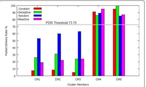
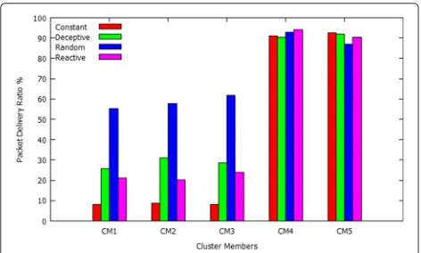
To illustrate the normal scenario and jamming scenario with different types of jammers, five set of samples of PDR are taken from the simulation results. In Figs. 3, 4, 5, 6, 7, and 8, theX-axis denotes the cluster members and the
Y-axis denotes PDR. The variety of color bars in Fig. 3 indicates different PDR samples (samples are taken from the simulation results) during normal scenario (when jam-mers are not introduced). From Fig. 3, it is evident that the PDR of every cluster members in the normal sce-nario is greater than the PDR threshold. Next, various jammers such as constant, deceptive, random, and reac-tive are introduced in the sensor network. The varieties of color bars in Figs. 4, 5, 6, and 7 indicate different types of jamming (constant, deceptive, random, and reactive). The simulation setup for this scenario is made in such a way that three CMs (CM1, CM2, and CM3) are affected by the jammer and two CMs (CM4 and CM5) are not affected by a jammer. The PDR distribution of cluster members during different types of jamming: with PDR threshold at 74.75 % and with the probability of 0.001 (Section 2.5.1), with PDR threshold at 77 % and with the probability of 0.01 (Section 4.3), with PDR threshold at 73.75 % and with the probability of 0.05 (Section 4.3), with PDR threshold at 62.5 % with the probability of 0.1 (Section 4.3) is shown in Figs. 4, 5, 6, and 7, respectively. From the figures, it is
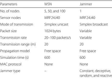
Table 10Simulation setup
Parameters WSN Jammer
No. of nodes 5, 50, and 100 1
Sensor nodes MRF24J40 MRF24J40
Mode of transmission Simplex unicast Simplex broadcast
Packet size 1024 bytes Variable
Transmission rate 20–100 packets/s Variable
Transmission range (m) 20 20
Propagation model Free space Free space
Simulation time (s) 600 600
MAC protocol None None
Jammer type – Constant, deceptive,
Fig. 3PDR distribution of CMs during the normal scenario. Representation of PDR distribution in cluster members (CM1, CM2, CM3, CM4, and CM5) during the normal scenario (sensor network does not include jammer). The PDR of CMs: CM1, CM2, CM3, CM4, and CM5, is above PDR threshold 74.75, 77, 73.75, and 62.5 % with probabilities 0.001, 0.01, 0.05, and 0.1, respectively
noted that the PDR of CM1, CM2, and CM3 in all the cases are lesser than the PDR threshold due to the influ-ence of jammer. But the PDR of CM4 and CM5 in all the cases are greater than the PDR threshold (because the members CM4 and CM5 are not jammed).
In Fig. 8, the average PDR of CM1, CM2, CM3, CM4, and CM5 for different types of jamming (constant, decep-tive, random, and reactive) with various probabilities is considered. From Fig. 8, it is evident that theoretically the constant jammer jams the entire transmission on the channel, since the constant jammer constantly injects the data packets on the communication medium. But in practice, negligible data transmission takes place. The data packets transmitted by CMs to CH are eradicated continuously by the constant jammer. Thus, the effect of jamming by the constant jammer is determined to
Fig. 4PDR distribution of CMs during various types of jamming with probability 0.001. Representation of PDR distribution in cluster members (CM1, CM2, CM3, CM4, and CM5) during various jamming with the probabilityp=0.001. The PDR of CMs: CM1, CM2, and CM3, is lesser than the PDR threshold 74.75 % and that of CM4 and CM5 is above PDR threshold 74.75 %
Fig. 5PDR distribution of CMs during various types of jamming with probability 0.01. Representation of PDR distribution in cluster members (CM1, CM2, CM3, CM4, and CM5) during various jamming with the probabilityp=0.01. The PDR of CMs: CM1, CM2, and CM3, is less than the PDR threshold 77 % and that of CM4 and CM5 is above PDR threshold 77 %
be above 90 % with respect to the average PDR of var-ious probabilities. The jamming effectiveness number is determined based on the averages over the resulting PDR percentage for the CMs: CM1, CM2, and CM3. The deceptive jammer jams the data transmission similar to constant jammer, but the deceptive jammer is aware of the existing protocol in the network. Therefore, the deceptive jamming effect is determined to be around 71 % with respect to average PDR of various probabilities. The data transmission is randomly jammed by the random jammer. The random jammer sleeps and jams the data transmis-sion at random time intervals. From the simulation result, it is noted that the random jamming effect is around 42 % with respect to average PDR of various probabilities. The reactive jammer is also aware of the communication protocol in the network like the deceptive jammer. The
Fig. 7PDR distribution of CMs during various types of jamming with probability 0.1. Representation of PDR distribution in cluster members (CM1, CM2, CM3, CM4, and CM5) during various jamming with the probabilityp=0.1. The PDR of CMs: CM1, CM2, and CM3, is less than the PDR threshold 62.5 % and that of CM4 and CM5 is above PDR threshold 62.5 %
reactive jammer listens to the transmission medium con-tinuously and initiates to jam the medium during data communication. The average effect of reactive jamming is shown around 80 % with respect to various probabilities.
From Fig. 8, it is evident that the constant jammer (with various probabilities) poses severe security thread than other jammers. But in reality, the sensor nodes and the jammers in the sensor network are limited with energy. Constant jammers will drain the battery quickly because of continuously injecting the data into the medium. Reac-tive jammer injects data packet to destroy the original data packet transmitted by the normal node. In contrast to constant jammer, the reactive jammer injects the data packet only when it senses the original data packet in the medium. Due to this, the lifetime of the reactive jammer with respect to energy consumption is certainly higher than the constant jammer. Therefore, from the attackers
Fig. 8The average PDR distribution of CMs with various types of jamming with various probabilities. Representation of average PDR distribution in cluster members (CM1, CM2, CM3, CM4, and CM5) with various probabilities 0.001, 0.01, 0.05, and 0.1
point of view, it is concluded that the reactive jammer (consumes energy only when the normal node is transmit-ting the data) is more effective than a constant jammer with respect to energy constraint.
4.3 Performance evaluation metrics
Generally, the CH identifies whether its members are in usual or unusual condition. The CH may not identify the member as in unusual condition or CH may inaccurately identify the CM as in usual condition. In order to detect the CMs accurately as in usual condition or in unusual condition, the detection of CMs may be categorized into (i) true detection, (ii) false detection, and (iii) undetection. The true detection is defined as CH that accurately detects the member as unusual when that member is jammed. The false detection is defined as CH that wrongly detects the member as unusual though that member is usual. The undetection is defined as CH that wrongly detects the member as usual although the member is actually jammed.
The factors that are used to compute the performance metrics, namely true detection ratio (TDR), false detec-tion ratio (FDR), and undetecdetec-tion ratio (UDR), are given as follows:
1. True positive indicator (TP) represents the number of accurately detected jammed members.
2. True negative indicator (TN) represents the number of accurately detected usual members, but the members are actually not jammed.
3. False positive indicator (FP) represents that the members are jammed but they are actually not jammed.
4. False negative indicator (FN) represents that the members are not jammed but they are actually jammed.
5. True positive ratio (TPR) is the number of accurately detected jammed members to the total number of members actually jammed.
6. True negative ratio (TNR) is the number of accurately detected usual members (members who are not jammed) to the total number of usual members. 7. False positive ratio (FPR) is the number of members
inaccurately detected as jammed to the sum of members who are detected as jammed and number of members who are actually not jammed.
8. False negative ratio (FNR) is the number of members inaccurately detected as usual to the sum of members who are detected as not jammed and the number of members who are actually jammed.
accurately detected by the CH to the number of mem-bers that are exactly affected by the jammer. The TDR is computed as follows:
TDR=TP/(TP+FN) (4)
FDR is defined as the ratio of the number of members that are inaccurately detected by the CH to the number of members that are not actually affected by the jammer. That is, a member is in usual condition but it has been wrongly detected as unusual. The FDR is computed as follows:
FDR=FP/(FP+TN) (5)
UDR is defined as the ratio of the number of members that are not detected by the CH to the number of mem-bers that are actually affected by the jammer. The UDR is computed as follows:
UDR=FN/(TP+FN) (6)
The JMR is defined as the ratio of the number of mem-bers successfully jammed by the jammer to the number of members falling within the coverage range of the jammer (number of members covered by the jammer). The JMR is computed as follows:
JMR=SJ/FJ, (7)
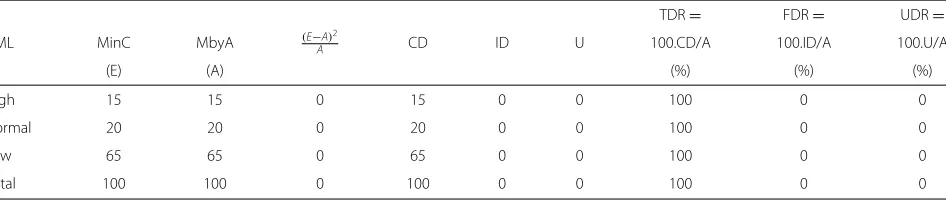
where SJ represents number of members successfully jammed by the jammer and FJ represents number of members falling within the coverage range of the jammer. The chi-square test is used to measure the performance difference between experimental values (from simulation results) and anticipated values. The chi-square test is applied after the simulations. A cluster of hundred mem-bers (CM1 to CM99 and CH21) is considered. The sim-ulation setup for this scenario is made in such a way that 15 members (CM1 to CM15) are affected by a jammer and the rest of the CMs are not affected by a jammer. The degree of freedom is calculated as 2 (as the number of groups are 3: normal, low, and high), and the level of sig-nificance is assumed to be 0.05 with the corresponding table value of 5.9915 for 95 % of confidence interval. The results are shown in Table 11 (result for one of the simula-tion is considered). In Table 11, CD denotes the members
correctly detected by JDF when the node is jammed, ID denotes the members who are incorrectly detected as abnormal by JDF when the node is in normal condition, and U denotes the members who are incorrectly detected as normal by JDF when the node is in abnormal condition. The result passes the chi-square test as the total under (E−A)2/Ais 0, which is lesser than the chi-square table value (5.991). Hence, there is no difference between the observed and anticipated values. The level of significance is 0.05. This states that the reliability of the result is 95 %, i.e., the obtained result is considered to be correct by 95 % and the chance of obtained result to be wrong by 5 %. Therefore, the result of the proposed system is significiantly encouraging.
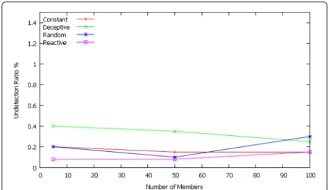
As discussed before, the PDR threshold value is fixed as 74.75 % (based on the result ofT test with the proba-bility of 99.9). Various types of jamming is launched. The TDR, FDR, and UDR are determined based on the PDR threshold (74.75 %). The mean TDR and FDR from these simulations are collected for different jammed members under various configurations for different types of jam-mers such as constant, deceptive, random, and reactive jammers. In the simulation, the configuration is changed by changing the total number of members in the cluster as 5, 50, and 100. Figs. 9, 10, and 11 show the values of TDR, FDR, and UDR for different types of jammers under various configurations with probability p = 0.001. This states that the reliability of the result is 99.9 %, that is, the obtained result is considered to be correct by 99.9 % and the chance of obtained result to be wrong by 0.1 %.
Similarly, theTtest is performed for other probabilities (p) such as 0.01, 0.05, and 0.1. The process of computing the t value for other probabilities is not included in the paper due to space constraint. However, the results are given as follows:
• T test is performed with four samples of PDR observed from members CM1, CM2, CM3, CM4, and CM5. The degree of freedom is computed as 3, and the level of significance is 0.01 with the correspondingt value being 5.9 for 99 % of
confidence interval. The result passes thet test. The t table value oft test is 5.84. From the observation, it is
Table 11Chi-square test result for one of the simulations
TDR= FDR= UDR=
GML MinC MbyA (E−AA)2 CD ID U 100.CD/A 100.ID/A 100.U/A
(E) (A) (%) (%) (%)
High 15 15 0 15 0 0 100 0 0
Normal 20 20 0 20 0 0 100 0 0
Low 65 65 0 65 0 0 100 0 0
Fig. 9TDR for different jamming of various configurations of p=0.001
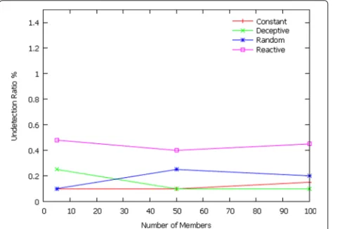
noted that thet value (5.9) exceeds the table value (5.84). This proves that there is significance and the PDR threshold is fixed as 77 %. Similar to the probability 0.001, the experiment is repeated for the probability 0.01. The mean TDR and FDR from these simulations are collected for different jammed members under various configurations for different types of jammers such as constant, deceptive, random, and reactive jammers. In the simulation, the configuration is changed by changing the total number of members in the cluster as 5, 50, and 100. Figs. 12, 13, and 14 show the values of TDR, FDR, and UDR for different types of jammers under various configurations with probabilityp=0.01. This states that the reliability of the result is 99 %, that is, the obtained result is considered to be correct by 99 % and the chance of obtained result to be wrong by 1 %. • T test is performed with four samples of PDR
observed from members CM1, CM2, CM3, CM4, and CM5. The degree of freedom is computed as 3, and the level of significance is 0.05 with the correspondingt value being 3.23 for 95 % of
confidence interval. The result passes thet test. The t
Fig. 10FDR for different jamming of various configurations of p=0.001
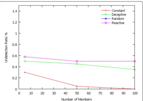
Fig. 11UDR for different jamming of various configurations of p=0.001
table value oft test is 3.18. From the observation, it is noted that thet value (3.23) exceeds the table value (3.18). This proves that there is significance and the PDR threshold is fixed as 73.75 %. Similar to the probability 0.01, the experiment is repeated for the probability 0.05. The mean TDR and FDR from these simulations are collected for different jammed members under various configurations for different types of jammers such as constant, deceptive, random, and reactive jammers. In the simulation, the configuration is changed by changing the total number of members in the cluster as 5, 50, and 100. Figs. 15, 16, and 17 show the values of TDR, FDR, and UDR for different types of jammers under various configuration with probabilityp=0.05. This states that the reliability of the result is 95 %, that is, the obtained result is considered to be correct by 95 % and the chance of obtained result to be wrong by 5 %. • T test is performed with four samples of PDR
observed from CMs CM1, CM2, CM3, CM4, and
Fig. 13FDR for different jamming of various configurations of p=0.01
CM5. The degree of freedom is computed as 3, and the level of significance is 0.1 with the corresponding t value being 2.39 for 90 % of confidence interval. The result passes thet test. The t table value of t test is 2.35. From the observation, it is noted that thet value (2.39) exceeds the table value (2.35). This proves that there is significance and the PDR threshold is fixed as 62.5 %. Similar to the probability 0.05, the experiment is repeated for the probability 0.1. The mean TDR and FDR from these simulations are collected for different jammed members under various configurations for different types of jammers such as constant, deceptive, random, and reactive jammers. In the simulation, the configuration is changed by changing the total number of members in the cluster as 5, 50, and 100. Figs. 18, 19, and 20 show the values of TDR, FDR, and UDR for different types of jammers under various configuration with probabilityp=0.1. This
Fig. 14UDR for different jamming of various configurations of p=0.01
Fig. 15TDR for different jamming of various configurations of p=0.05
states that the reliability of the result is 90 %, that is, the obtained result is considered to be correct by 90 % and the chance of obtained result to be wrong by 10 %.
Initially, the PDR threshold (PDR Threshold) is fixed based on the result of theTtest discussed in Section 2.5.2. The PDR Threshold is fixed as 74.75, 77, 73.75, and 62.5 % for the confidence levels at 99.9, 99, 95, and 90 %, respec-tively. The proposed JDF is simulated based on various PDR Thresholds and RSSI Threshold, for measuring the performance in terms of performance evaluation metrics (TDR, FDR, and UDR). From the results, it is observed that the proposed system with confidence levels at 99.9, 99, and 95 % detect all types of jamming and the proposed system with confidence level at 90 % detects constant, deceptive, and reactive jammings and does not detect random jamming. It is also noted that among chosen con-fidence level for simulation, the proposed system with
Fig. 17UDR for different jamming of various configurations of p=0.05
confidence level at 99 % works well (TDR = 99.8 % and FDR=UDR=0).
Now, the performance evaluation metrics of the proposed system is compared for confidence level at 99 % with the existing system [8]. From Table 12, it is noted that the proposed system for confidence level at 99 % works better than the existing system. The reliability of the proposed system result is 99 %. That is, the obtained result is considered to be cor-rect by 99 % and the chance of obtained result to be wrong by 1 %. The proposed system for confidence level at 99 %.
To the best of our knowledge, none has considered jammer intrusion detection and jamming detection in the cluster-based WSN. But research work on jammer and jamming detection are carried out in other kinds of net-work such as IEEE 802.11b wireless netnet-work [23], IEEE 802.11 network [24], and IEEE 802.11 wireless LAN [25]. This lies as the motivating factor behind the design and
Fig. 18TDR for different jamming of various configurations ofp=0.1
Fig. 19FDR for different jamming of various configurations ofp=0.1
implementation of proposed JDF. However, in order to provide a holistic research insight on jammer and jam-ming detection, the proposed JDF is compared with recent research works on jammer and jamming detection in other modern networks as given in Table 13.
4.4 Energy consumption
Theoretical- and simulation-based energy consumption analyses of JDF are performed, and these analyses are bases to evaluate the trade-off within a WSN. The the-oretical energy consumption analysis incudes (i) analysis on energy consumption in the normal scenario, (ii) analy-sis on energy consumption on jammer intrusion detection (JID), and (iii) analysis on energy consumption on jam-ming detection (JD).
Analysis on energy consumption based on theoretical model:
In sensor network, the node’s energy is consumed due to data packet transmission, data packet reception, and computations performed by nodes. Theoretical energy