2017 2nd International Conference on Artificial Intelligence: Techniques and Applications (AITA 2017) ISBN: 978-1-60595-491-2
Target Localization Based on Invariant Image Features
Bo LEI
Science and Technology on Electro-Optic Control Laboratory, Luoyang 471009, China
Keywords: Image matching, Invariant features, Target locating.
Abstract. Distinctive invariant features from images are perform reliable to image scale and rotation, also applicable to change in 3D viewpoint, so it is widely used in image matching and target locating. This paper analyses the extracting theory and process of invariant features from images in detail, and presents a method that can be used to calculate transforming modulus between two images are according to invariant features, finally accomplishing the target locating, which exist in two images together. Simulation results indicate that the paper method have excellent performance in target locating, it is precision for target locating between two images based on invariant features from images.
Introduction
Usually, we need locating coordinate of the target between two images which one is called based image, another is called real-time image with image matching in precision bombing in operation, which is a fundamental aspect of many problems in computer vision, including object or scene recognition, solving for 3D structure form multiple images, stereo correspondence, and motion tracking.
The task of finding correspondences between two images of the same scene or object is the most import part of image matching, we chose a high level set of natural visual features of the interest point in the image as discrete image correspondences, such as corners, blobs, and T-junctions.
There are many ways to detect interest point in the image. The most widely used detector probably is the Harris corner detector[2], proposed back in 1988, based on the eigenvalues of the second-moment matrix. However, Harris corners are not scale-invariant. Lindeberg introduced the concept of automatic scale selection. This allows to detect interest points in an image, each with their own characteristic scale. He experimented with both the determinant of the Hessian matrix as well as the Laplacian (which corresponds to the trace of the Hessian matrix) to detect blob like structures. Mikolajczyk and Schmid refined this method, creating robust and scale-invariant feature detectors with high repeatability, which they coined Harris-Laplace and Hessian-Laplace[3]. They used a (scale-adapted) Harris measure or the determinant of the Hessian matrix to select the location, and the Laplacian to select the scale.
SIFT was developed by Lowe[4] for image feature generation in object recognition applications. The features are invariant to image translation, scaling, rotation, and partially invariant to illumination changes and affine or 3D projection. These characteristics make them suitable landmarks for robust matching when the cameras are moving around in an environment, as the landmarks are observed from different angles, distances or under different illumination.
The SIFT features are determined by identifying repeatable points in a pyramid of scaled images. Feature locations are identified by detecting maxima and minima in the Difference-Of-Gaussian pyramid. A subpixel location, scale and orientation are associated with each SIFT feature.
In the next section, we introduce the SIFT algorithm in detail. In section IV, we give an approach of locating target coordinate by SIFT. In section V, we present simulation results of the proposed method.
Interest Point Detector
Scale-space Foundations
If we describe some phenomena in different resolution and research them in dynamic resolution, then some cell information will be discovered, which can not be knew in tradition ways. In the field of image processing this method is called Scale-space model.
It has been shown that under a variety of reasonable assumptions the only possible scale-space kernel is the Gaussian function. Therefore, the scale space of an image is defined as a function that is produced from the convolution of a variable-scale Gaussian, as
) , ( * ) , , ( ) , ,
(x y G x y I x y
L σ = σ (1)
2 2 2 2 2 2
1 ) , , (
G σ
πσ σ
y x e y
x
+
= (2) Where I( yx, ) is an input image, σ is the factor of scale. The discrete function is
)
,
(
)
,
,
(
)
,
,
(
1 2 1 21 2
k
j
k
i
I
k
k
G
j
i
L
m
m k
m
m k
−
−
=
∑ ∑
−
= =−
σ
σ
(3)Because of the Gaussian function can restrain affect all of image pixels between3σ, the paper use ]
4 [ σ =
m to simulate so that it can reduce the cost of computation.
To efficiently detect stable keypoint locations in scale space, we can use scale-space extrema in the difference-of-Gaussian function convolved with the image, D(x,y,σ), which can be computed from the difference of two nearby scales separated by a constant multiplicative factor k.
) , , ( ) , , ( ) , ( * )) , , ( ) , , ( ( ) , ,
(x y σ G x y kσ G x y σ I x y L x y kσ L x y σ
D = − = − (4)
Detection of Scale-space Exterma
Maxima and minima of the difference-of-Gaussian images are detected by comparing a pixel to its 26 neighbors in 3x3 regions at the current and adjacent scales. It is selected only if it is larger than all of these neighbors or smaller than all of them.
The Reject Unstable Keypoints
These exterma points are candidate keypoints, which need to be rejected that have low contrast( and are therefore sensitive to noise) or are poorly localized along an edge. we use the Taylor expansion (up to the quadratic terms) of the scale-space function to reject the unstable keypoints:
xxxx xxxx xxxx 2222 1111 xxxx xxxx
xxxx 2222
∂ ∂ +
∂ ∂ + =
= D x y D D D
D( ) ( , ,σ) T T 2 (5)
4 / )) , , 1 ( ) , , 1 ( ) , , 1 ( ) , , 1 ( ( ) , , ( 2 ) , , ( ) , , ( ) , , ( 2 ) , , 1 ( ) , , 1 ( 2 / )) , , ( ) , , ( ( 1 1 1 1 2 1 1 2 2 2 2 1 1 + − − + − + − + − − + − − + + = ∂ ∂ ∂ − + = ∂ ∂ − − + + = ∂ ∂ − = ∂ ∂ k k k k k k k k k y x D y x D y x D y x D x D y x D y x D y x D D y x D y x D y x D x D y x D y x D D σ σ σ σ σ σ σ σ σ σ σ σ σ σ σ (6)
Taking the derivative of (5) with respect to x and setting it to zero, giving:
xxxx xxxx xxxx ∂ ∂ ∂ ∂ − = − D D 2 1 2
ˆ (7) Then substituting (7) into (5), giving:
1 ˆ ( ) 2 T D D =D+ ∂
∂
x x
x (8) )
(xxxx
D can be used for rejecting unstable extrema with low contrast, which all extrema with a value of D(xxxx)less than 0.03 were discarded.
The difference-of-Gaussian function have a strong response along edges, therefore it is needed to reject unstable keypoints of strong response along edges. The eigenvalues of the 2×2Hessian matrix are proportional to the principal curvatures of D(xxxx). Let
α
be the eigenvalue with the largest magnitude and β be the smaller one. We can avoid explicitly computing the eigenvalues, as we are only concerned with their ratio. Let rbe the ratio, r αβ = then:
2 2 2 2
2
( ) ( ) ( ) ( 1)
det( )
tr H r r
H r r
α β β β
αβ β
+ + +
= = = (9) Therefore, to check that the ratio of principal curvatures is below some thresholdr, we only need to check:
2 2
( ) ( 1)
det( ) tr H r
H r
+
< (10) The experiments in the paper use a value of r=10, which eliminates keypoints that have a ratio between the principal curvatures greater than 10:
2 2 2
( ) ( 1) (10 1)
det( ) 10
tr H r
H r
+ +
≥ = (11) Up to now, the stable keypoints have been obtained.
Keypoints Matching
around the interest point and stores the bins in a 128-dimensional vector (8 orientation bins for each of the 4 × 4 location bins). So a keypoint descriptor is a 128-dimensional vector.
Then, the descriptor vectors are matched between different images. The matching is based on a Euclidean distance between the vectors:
∑
=
− =
128
1
2 ) (
i i i
d α β (12) where α,β is the keypoint descriptor vector of two images, d is the Euclidean distance.
Application
When we accomplish image matching between different images, we need locating the target coordinate so that we can implement automated target recognition and track. It can be achieved to compute the transform parameter between two images.
An amount of SIFT keypoints can be detected in the image and the features are invariant of scaling, rotation, translation, so we present a method for computing the transform parameter between two images with SIFT matching keypoints to accomplish locating the target.
It is defined that (x0,y0)is the based image coordinate and ( yx, ) is the real-time image coordinate, so
23 0 22 0 21
13 0 12 0 11
T y T x T y
T y T x T x
+ +
=
+ +
=
(13) We chose three pairs coordinate of the right match keypoints to computer transform parameter:
) , ( ) ,
(x01 y01 → x1 y1 ,(x02,y02)→(x2,y2),(x03,y03) →(x3,y3). The equation (14) shows
the method:
=
=
23 22 21
03 03
02 02
01 01
3 2 1
13 12 11
03 03
02 02
01 01
3 2 1
1 1 1
1 1 1
T T T
y x
y x
y x
y y y
T T T
y x
y x
y x
x x x
(14)
Simulation and Analysis
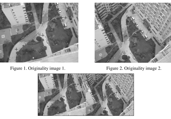
We can select two images of 314×235, as shown in figure 1 and figure 2. Obviously, they have translation, rotation, zoom relationship to a certain extent, and little perspective. We select 4 keypoints in figure 1, and we can get 4 targets in figure 2 by SIFT image matching to calculate the transpositional parameter. The simulation result is shown in figure 3.
There are four targets in figure 1, but we only get three in figure 2, because one of the targets in figure 1 does not exist in figure 2.
The simulation result shows that:
1) The target can be located precisely using transpositional parameters calculated by SIFT keypoints. However, the aberration between two images will cause locating error.
Figure 1. Originality image 1. Figure 2. Originality image 2.
Figure 3. Simulation result.
Conclusion
This paper presented a method for extracting distinctive features from images, and this can be used to match between images which have translation, rotation, zoom and little perspective relationship. This paper has also presented a method of target locating by invariant features which extracting from SIFT algorithm. The simulation result shows that SIFT keypoints have outstanding matching performance, and can be used for precisely target locating.
References
[1] Moravec H, “Rover Visual obstacle avoidance [C],” International Joint Conference on Artificial Intelligence, 1981, pp. 785-790.
[2] Harris C, Stephens M, “A combined corner and edge detector[C]”, Fourth Alvey Vision Conference, l988, pp. 147-151.
[3] H. Bay, T. Tuytelaars, L. Van Gool, “SURF: Speeded up robust features”, ECCV, 2006, Vol. 1, pp. 404-417.
[4] Lowe D G, “Distinctive image features from scale—invariant keypoints[J]”, International Journal of Computer Vision, 2004, 60(2), pp. 9l-ll0.
[5] Helmer S, LoweD G, “Object recognition with many local Features[C]”, Workshop on Generative Model Based Vison 2004(GMBV), 2004.
[6] Lowe D G, “Object recognition from local scale-invariant features[C]”, International Conference on Computer Vision, 1999. pp. 1150-1157.