Thesis by
Zhipu Jin
In Partial Fulfillment of the Requirements for the Degree of
Doctor of Philosophy
California Institute of Technology Pasadena, California
2007
c
2007
Acknowledgements
First of all, I would like to express my heartfelt gratitude to my advisor, Prof. Richard M. Murray, for his guidance that is so conducive to the work I have undertaken. His broad knowledge, deep insights, outstanding leadership, and great personality make him a mentor that every student dreams of having. I am grateful to my committee members: Prof. John C. Doyle, Prof. Joel W. Burdick, Prof. Babak Hassibi, and Prof. Tracey Ho, for inspiring discussions and detailed comments on my thesis. I also appreciate the help from Prof. Michelle Effros, Prof. Leonard Schulman and Prof. Steven Low.
There are many other people I would like to acknowledge with thankfulness for the help given to me in the last five years. Thanks to Dr. Alcherio Martinoli for the unforgettable support during my first year at Caltech. Thanks to Dr. Reza Olfati-Saber for showing me his wonderful work on coordinated control. Thanks to Dr. Eric Klavins, Dr. Lars Cremean, David van Gogh, and Steve Waydo for helping me conduct experiments on the testbed. Also, thanks to Vijay Gupta, Ling Shi, Abhishek Tiwari, and other group members for collaborations and brainstorming. Because of them, my research became much easier and more fruitful. Also thanks to staffmembers at Caltech for making my administrative life easy.
I would like to thank Lijun Chen, Xiaoli Feng, Hao Jiang, Lun Li, Yongqiang Liang, Xin Liu, Changlin Pang, Zhengrong Wang, Qiang Yang, Chengzhong Zhang, Kechun Zhang, Yizhen Zhang, and all other friends I made here. Thanks to them for bringing me so many enjoyable memories.
Abstract
Coordination in networked multi-agent systems attracts significant interest in the realm of engineering. Typical examples include formations of unmanned aerial vehicles, auto-mated highway systems, and sensor networks. One common feature for these systems is that coordinated behaviors are exhibited by interactions among agents where information exchange and manipulation are necessary. In this work, three relevant issues are investi-gated in detail: uniform strategy for multi-agent formation control, fast-converging con-sensus protocols, and packet-based state estimation over communication networks.
Formation control of multi-agent systems involves harmony among local controller de-sign, interaction topology analysis, and objective agreement among networked agents. We propose a novel control strategy so that each agent responds to neighbors’ behaviors as well as acts towards the global goal. Thus, information flows for local interactions and global objective synchronization are studied separately. Using the tools from signal flow graphs and algebraic graph theory, we show that this new strategy eases the design of local controllers by relaxing stabilizing conditions. Robustness against the link failure and scal-able disturbance resistance are also discussed based on small-gain theory. Experimental results on the Caltech multi-vehicle wireless testbed are provided to verify the feasibility and efficiency of this control strategy.
Contents
Acknowledgements iv
Abstract v
1 Introduction 1
1.1 Background and Motivation . . . 1
1.2 Previous Work . . . 4
1.2.1 Multi-Agent Formation Control . . . 4
1.2.2 Collective Behaviors and Consensus Seeking . . . 7
1.2.3 Control and Estimation over Networks . . . 8
1.3 Statement of Contributions . . . 11
2 Preliminaries 13 2.1 Algebraic Graph Theory . . . 14
2.1.1 Basic Concepts . . . 14
2.1.2 Matrices in Algebraic Graph Theory . . . 15
2.1.3 Infinity Norm of Normalized Adjacency Matrix . . . 21
2.2 Quantization and Distortion . . . 24
2.3 Modeling for Packet Drops . . . 26
3 Double-Graph Control Strategy for Formation Control 29 3.1 Formulation of Double-Graph Control Strategy . . . 29
3.1.1 Gain Matrix in Signal Flow Graphs . . . 29
3.1.3 Double-Graph Control Strategy . . . 35
3.2 Stability Analysis for Double-Graph Control Strategy . . . 38
3.3 Performance for Double-Graph Control Strategy . . . 43
3.3.1 Disturbance Resistance with Acyclic Interaction Topologies . . . . 44
3.3.2 Disturbance Resistance with Arbitrary Interaction Topologies . . . 45
3.3.3 Other Performance Issues . . . 47
3.4 Simulation and Experimental Results . . . 48
3.4.1 Multi-Vehicle Wireless Testbed . . . 48
3.4.2 Simulation Results . . . 50
3.4.3 Experimental Results . . . 52
4 Consensus Protocols in Networked Multi-Agent Systems 57 4.1 Consensus Seeking for Multi-Agent Systems . . . 57
4.2 Multi-Hop Replay Protocols for Consensus Seeking . . . 63
4.2.1 Two-Hop Relay Protocol . . . 64
4.2.2 Convergence Speed of Two-Hop Relay Protocol . . . 66
4.2.3 Multi-Hop Relay Protocol . . . 67
4.3 Two-Hop Relay Protocols with Time Delays . . . 67
4.4 Examples and Simulation Results . . . 73
5 Packet-Based State Estimation Using Multiple Description Codes 78 5.1 Formulation and Assumptions for Packet-Based State Estimation . . . 79
5.2 Multiple Description Source Codes . . . 81
5.2.1 Theoretical Limits of Multiple Description Codes . . . 83
5.2.2 Multiple Description Scalar Quantizer . . . 84
5.2.3 Quantization Noise of MD codes . . . 86
5.3 Kalman Filtering Utilizing MD Codes . . . 87
5.3.1 Kalman Filtering with i.i.d. Packet Drops . . . 87
5.3.2 Discussion for Generalized MARE . . . 98
5.3.3 Kalman Filtering with Bursty Packet Drops . . . 100
6 Conclusions and Future Work 110 6.1 Summary of Main Contributions . . . 110 6.2 Future Directions and Possible Extensions . . . 112
Bibliography 115
A Index Assignment Method for MDSQ 129
List of Figures
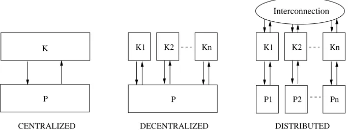
1.1 Architectures for centralized, decentralized, and distributed control
architec-tures . . . 1
1.2 Diagram of a typical networked control system . . . 9
2.1 Classification for directed graphs . . . 15
2.2 An example: directed graph with seven vertices . . . 17
2.3 Reduction of a directed graph . . . 20
2.4 Bounds of normalized adjacency matrix norm . . . 24
2.5 Models of packet drops: (a) i.i.d. Bernoulli model; (b) two-state Markov chain model . . . 27
3.1 A signal flow graph . . . 29
3.2 Interaction topology and the corresponding signal flow graph . . . 34
3.3 Double-graph control strategy for multi-agent systems . . . 37
3.4 Diagram of the local control strategy . . . 38
3.5 Interaction topology of a leader-follower system with twelve agents . . . 39
3.6 Nyquist plot and critical points . . . 40
3.7 Mapping for critical points . . . 41
3.8 Ellipses for critical points with differentα . . . 42
3.9 Nyquist plot and critical points for double-graph control strategy . . . 42
3.10 Disturbance for single agent . . . 44
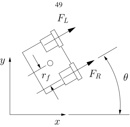
3.11 Schematic plot of MVWT vehicle. . . 49
3.12 Control diagram for lateral dynamics. . . 51
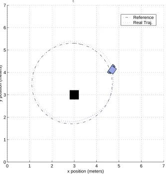
3.14 Top view of a single vehicle experiment . . . 53
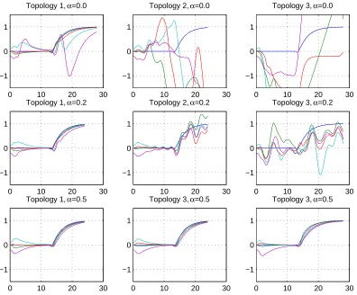
3.15 Lateral errors for vehicle formation with different parameters . . . 54
3.16 Topologies in double-graph control strategy of the MVWT experiment . . . . 54
3.17 Top view of vehicle formation experiment . . . 55
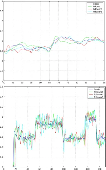
3.18 Vehicle formation experiment: radius and speed . . . 56
4.1 A directed graph and its two-hop directed graph . . . 64
4.2 An example of disconnected two-hop directed graph . . . 67
4.3 Locus of the zero of the quasipolynomial and the generalized eigenvalue . . . 71
4.4 Three different topologies: G1,G2, andG3 . . . 73
4.5 States of graphG2with no delay . . . 75
4.6 States of graphG2with delayτ= 0.038 . . . 75
4.7 States of graphG2with delayτ= 0.05 . . . 76
4.8 States of graphG2with delayτ= 0.25 . . . 76
4.9 Tradeoffbetweenλ2andτ∗ . . . 77
5.1 Diagram of packet-based state estimation . . . 80
5.2 Diagram of two-description MD source encoder . . . 85
5.3 Additive noise model of uniform scalar quantization . . . 86
5.4 Simulation results of expected error covariances with theoretical upper and lower bounds . . . 105
5.5 Mean values of error covariance with same central distortions . . . 106
5.6 Mean values of error covariance with same bpss . . . 107
5.7 Mean values of error covariance with low dropping rate . . . 107
5.8 Theoretical upper and lower bounds for burst packet-dropping case with q11 =95% . . . 108
5.9 Simulation results for burst packet-dropping case . . . 109
A.1 Two actions to fill the index mapping matrix . . . 130
List of Tables
Chapter 1
Introduction
1.1
Background and Motivation
As an engineering discipline, automatic control theory is always tied to practical prob-lems encountered in human history. Classical control theory relies on transform methods in the frequency domain to deal with single-input-single-output (SISO) systems. Starting in 1960’s, the state-space method has been used for multiple-input-multiple-output (MIMO) systems. Efficient algorithms for solving matrix equations and advanced microprocessors for data processing popularize this time-domain approach. However, for large scale con-trol objects, such as electric power grids or large oil refineries, thousands of signals and variables need to be sensed and calculated. The lack of full sensor information and limited computation capability make the conventional centralized methods fail.
K1 K2 Kn
P K
P
K1 K2 Kn
P1 P2 Pn DECENTRALIZED DISTRIBUTED CENTRALIZED
[image:13.595.154.496.514.645.2]Interconnection
Figure 1.1: Architectures for centralized, decentralized, and distributed control architec-tures
numer-ous efforts has been made [1]. Three different control architectures for large scale systems are shown in Figure 1.1. For the first architecture, a centralized controller K is used to con-trol a dynamic system P. One direct way to solve the complexity crisis is model reduction (or model simplification) [2, 3, 4]. This approach tries to reduce the order of state space by simplifying the system structure so that the complexity of the central controller can be moderated.
The second architecture in Figure 1.1 decentralizes the feedback controller. Instead of using one centralized controller, which requires full (or controllable) state feedback, spatially separated controllers{K1,K2,· · · ,Kn} are introduced. Generally, each controller
only accesses part of the system states and there are no information exchanges among the controllers. The most definitive results on decentralized stabilization can be found in [5, 6]. Note that the term “decentralization” refers to controller implementation and the control law is designed in a centralized mode.
The third architecture is a distributed control architecture where control object is com-posed of multiple decoupled subsystems{P1,P2, . . . ,Pn}. Each subsystem is equipped with
a local controller. Interconnection exists among these controllers so that information can be exchanged and subsystems can interact with each other. Thus, distributed control laws are generated according to not only the local feedback, but also the messages from other con-trollers. Cooperative and coordinated control for networked multi-agent systems belongs to this structure.
[10, 11, 12].
During the last few decades, cooperative and coordinated control for multi-agent sys-tems has received significant attention. Dramatic developments in communication and computation technology relax the restrictions on information exchanges between spatially distributed agents. The possibility has been identified that simple and inexpensive agents can carry out complicated tasks through collaboration that may be too difficult for single agent. Advantages include simple structure, low cost, enhanced functionality, and the flex-ibility in fault tolerance. Applications of cooperative and coordinated multi-agent systems can be found in space exploration [13, 14, 15, 16, 17, 18, 19], automated highway sys-tems [20, 21, 22, 23, 24, 25], autonomous combat syssys-tems [26, 27, 28], oceanographic sampling [29, 30, 31], air traffic control [32, 33], congestion control on the internet [34], and sensor networks [35, 36, 37]. An agent can represent a spaceship, an airplane, a ground/underwater vehicle, an internet router, a cellular phone, or even a smart sensor with microprocessors. Among these applications, a couple of issues have not yet been well answered:
• Interactions among agents make the dynamics of multi-agent systems more compli-cated than single agent. Practical design and implementation needs more constructive insights from qualitative analysis on stability and performance issues with respective to nontrivial agent dynamics and interaction topology.
• Agents are physically decoupled. But their behaviors are coupled though a certain task that they try to accomplish. Task decomposition and assignment are traditionally solved in a centralized manner. Their counterparts in distributed systems, which can avoid the complexity crisis, are still not fully addressed.
In order to conquer these challenges, developing new tools and techniques from the interdisciplinary territory of control, computation, and communications is necessary [38]. A short survey of recent related work is provided in the next section, which obviously is bounded by author’s ignorance and biases. But, it is clear that control theory can definitely benefit from other closely related disciplines, such as graph theory, distributed computa-tion, information theory, and networking analysis. This work is dedicated to presenting our recent work on coordinated control for networked multi-agent systems, which can be roughly divided into three topics: coordinated control strategy for networked multi-agent systems, multi-hop relay protocols that boost the process of consensus seeking, and packet-based state estimation over lossy communication networks.
1.2
Previous Work
1.2.1
Multi-Agent Formation Control
Formation control is a popular topic for multi-agent systems. The control objective is letting agents maintain certain geometric formation by autonomously responding to other agents and the environment. Formation control has been extensively investigated in nu-merous applications such as coordination of multiple robots [39, 40, 41, 42, 43], control of ground vehicle platoons [22, 23, 25], formation flight of unmanned aerial vehicles (UAVs) [26, 27, 28, 44], fleets of autonomous underwater vehicles (AUVs) [30, 31, 45], and satel-lite clusters [15, 16, 19]. Even though each application shows unique characteristics and challenges, there exist common features. In most of the applications, agents have identical dynamics and similar local controller structure. Also, communication and computation ca-pacity for each agent is limited. Last, formation configurations are consistent with the third architecture in Figure 1.1, and the interaction topology plays an important role.
Various approaches for formation control have been proposed and they can be roughly categorized as the leader-follower approach, the virtual structure approach, and the behavior-based approach.
followers who try to follow the leader’s behavior by reacting to their nearest neigh-bors. This approach is naturally implemented in a distributed pattern since each agent only needs to react to its local environment. However, there exist a couple of short-comings. For example, the approach heavily depends on the leader status and the whole formation will fail if the leader fails. Also, the stability of single agent does not necessarily indicate the stability of the formation [46]. Thus, more critical stable conditions have to be posed on the local controller. Moreover, nontrivial agent dy-namics results in disturbance accumulation, which is unscalable with respect to the number of agents [23].
• The virtual structure approach is commonly used in the robotics community [47, 39, 45, 48, 49]. The unique feather is that a “virtual” agent is synthesized based on all agents. The formation is treated as a rigid body and this fictitious agent acts as the reference. The position and trajectory of each other agent is calculated explicitly based on the reference and formation configuration. It is easy to describe the whole group and maintain accurate formation. However, this approach is only practical for small groups because centralized data collection and processing are needed. Recent attempts on distributed implementation are reported in [18, 50].
• In the behavior-based approach, the control law of each agent is defined by a combi-nation of pre-defined control actions corresponding to all possible agent status. Even through this approach is distributed, it is difficult to analyze quantitatively. Limited applications for this approach are reported in [40, 51].
Obviously, formation control belongs to the distributed architecture. For agent Pi, we
can present its dynamics as
˙xi = f
xi,ui(xi,xneighbor)
,
(1.1) where xneighbor is the information collected from the neighbors and determined by the in-teraction topology. The local controller Ki generates the control law ui(xi,xneighbor). When
a mathematic theory on the properties of graphs. The objects of graph theory are a set of vertices and the edges between them. The idea of using graphs to interpret the interaction topologies can be found as early as in [53], where the input-output stability is decomposed into the stability of a hierarchy of strongly connected subsystems. For formation control, each agent can be abstracted as a vertex, and edges are used to present the existence of interactions. In [39, 40], graphs are used for the virtual structure of mobile robots. In [41], a triplet of leader robot, formation shape variable, and control graph is introduced for path planning and formation control of nonholonomic robots. Specific graphs, such as strings, are used in coordinated control for vehicle platoons [22]. In these literatures, stability of the formation is straightforward either because of the trivial agent dynamics or the simplicity of the graph.
For interaction topologies with loops, formation stability becomes tricky. A branch of graph theory, algebraic graph theory, is especially beneficial because of its fruitful results on graphs in connection with linear algebra. In [54, 55], spectrum analysis of the Laplacian matrix, a subject in algebraic graph theory, is shown to be important for the synchroniza-tion of coupled oscillators. Lyapunov stability analysis in terms of the eigenvalues of the Laplacian matrix is reported in [56] for nonlinear systems. A more precise statement on formation stability with linear dynamics is presented in [46]. It has been shown that the formation stability is equivalent to the stability of a sequence of decoupled inhomogeneous subsystems.
Another issue for formation control is the disturbance accumulation phenomenon. A disturbance signal can be amplified when it propagates to other agents through interactions. This subject is identified as the “string stability” problem in [22, 23] where formation con-trol of vehicle platoons is discussed. In order to bound this amplification, numerous designs for interaction topology are proposed. The results are extended to vehicle formation with mesh topologies [25]. The point is to weaken the coupling among vehicles so that the gain of the disturbance is less than 1.
flow has been widely used and well understood. However, because of the ignorance of the global objective, coordination between agents is often naive and undirected. With popular-ization of affordable wireless communication networks, it is possible to process and spread the global information in a distributed fashion using collective protocols. Thus, a uniform framework is needed to fully understand the formation control of networked multi-agent systems under the influence of local and global information flow.
1.2.2
Collective Behaviors and Consensus Seeking
Self-organizing features in animal groups, such as flocking, swarming, and schooling [57, 58], provide important insights for coordinated control in multi-agent systems. Theo-retical discussions can be found in [59] for the self-driven particles alignment problem, in [60] where a continuum mechanics approach is used, and in [61] for rotating swarms with all-to-all interactions.
As we mentioned in the previous section, the traditional architecture for global infor-mation processing normally involves centralized inforinfor-mation collection and computation. Surprisingly, collective algorithms provide possible distributed solutions for the same prob-lem. A good example is average consensus seeking. Driving the states of all agents to a common value by distributed protocols based on a communication network is called the consensus problem. A popular discrete-time consensus protocol is proposed in [62] based on stochastic matrix theory [63]. Suppose xi is the state of agent i and the protocol can be
summarized as
xi(k+1)=
j∈N(i)∪{i}
αi j(k)xj(k) (1.2)
where N(i) represents the set of agents whose state is available to agent i at step k. We assumeαi j ≥ 0 and jαi j(k) = 1. In other words, agent state is updated as the weighted average of its current value and its neighbors’. Correspondingly, a continuous-time con-sensus protocol can be found in [64, 65] as
˙xi(t)= −
j∈N(i)
where βi j(t) denotes the positive weight. We say the system has achieved a consensus if xi −xjconverges to zero as t → ∞for any i j. More specifically, it is called average
consensus when xi →
xi(0)/n as t→ ∞for any i where n is the number of agents.
Suppose the topology of the communication network is time-invariant. The necessary and sufficient condition for consensus protocol (1.2) and (1.3) to reach a consensus is that there exists a spanning tree in the topology [66, 67]. For average consensus seeking, the topology must be at least strongly connected and balanced [64]. When the topology is time-variant, such as in an ad-hoc wireless network, it has been shown that consensus protocols are still valid under switching topologies given the condition that at least one topology is strongly connected [65] or there exists a spanning tree [67] in each uniformly bounded time interval. The impact of communication delays on consensus seeking are also studied in [64, 68] where upper bounds of the delay margin are given for a fixed communication topology with uniform delay.
Consensus protocols has been employed in many engineering problems. For coordi-nated control, consensus schemes have been applied to achieve vehicle formations [66]. In rendezvous problems, consensus seeking is applied to control agents arrive at a certain lo-cation simultaneously [69]. Other applilo-cations include spacecraft attitude alignment [51], distributed decision making [70], asynchronous peer-to-peer networks [71], and robot syn-chronization [72]. All of these applications rely on the assumption that the convergence speed of consensus seeking is fast enough. A couple of methods have been reported to improve the convergence speed, such as finding the optimal weights associated with every communication link [37] or using random rewiring to change the topology [73], but they all face difficulties in practical implementation.
1.2.3
Control and Estimation over Networks
Dynamic System
Network 1 Communication
State Estimator
Encoder
Decoder Controller
Communication Network 2
Encoder
Decoder Observer
Figure 1.2: Diagram of a typical networked control system
In the structure of the NCS, a couple of fundamental assumptions for conventional control theory are not valid anymore due to the “imperfect” data links. For example:
• Infinite bandwidth. The communication channel can only transmit the data with cer-tain precision under the constraint of limited bandwidth. Quantization and distortion must be considered for system design and analysis.
• Reliable connections. Sampled signals are transmitted in data packets that suffers from unreliability issues such as unpredictable transmission delays and random packet drops.
• Static structure. For networked multi-agent systems, dynamic routing and ad-hoc connectivity of modern communication networks makes the interaction topology time-variant and the coupling among agents may change as well.
Several of related research threads exist to accommodate these issues. One thread is designing communication protocols and algorithms that minimize the probability of net-work congestion and packet drops [74]. Another one is treating these issues as additional constraints. For example, the maximum allowable transfer interval is discussed in [75] for desired stability and performance. Methods to compensate for network-induced delays are presented in [76]. In [77], a “recursive state estimator” is used to generate minimum variance estimates in the presence of irregular communication delays.
con-straints.” Under the framework of NCS, many significant results are reported. The esti-mation and stabilization problem of a closed-loop dynamic system over a communication channel with finite bandwidth is first discussed in [78, 79]. The necessity of a unified ap-proach to control, communication, and computation is emphasized in [80]. Quantization issues are discussed in [81]. In [82], an optimal algorithm quantizer, the “logarithmic quan-tizer”, is introduced in order to minimize the transmission bits. After that, a lower bound of the channel capacity needed to stabilize a linear time-invariant (LTI) system is given in [83]. Also, simple time-variant coding schemes are proposed for noiseless and noisy channels in [83] and [84], respectively. In [85], a concept of anytime capacity is proposed to deal with the real-time issue in NCS. Moreover, the authors for [86] try to address the stability of NCS in a stochastic way by introducing the concept of “almost-sure stability.”
For the model-based estimation problem, a popular method for linear systems is Kalman filtering [87, 88]. For a nonlinear system, an extended Kalman filter is a natural choice. In recent years, the moving horizon estimation approach [89] has become another promising method by transferring the estimation problem to a nonlinear optimization problem within a finite horizon time interval and solving it on-line. In NCS, the input data of estimator is disordered or intermittent because of the transmission delays or packet drops. Studies on filtering with intermittent observations can be tracked back to [90] and [91]. Other researchers try to model the Kalman filter with missing observations as jump linear sys-tems (JLS), which are stochastic hybrid syssys-tems with linear dynamics and discrete Markov chains. Certain convergence criteria are given for expected estimation error covariance [92, 93].
1.3
Statement of Contributions
Contributions of this work are briefly stated in following paragraphs, which are sorted by chapter and provide an outline of the thesis.
Chapter 2 In this chapter, we review some basic concepts and ideas from algebraic graph theory. Preliminary results about the spectrum and infinity norm of the Laplacian matrix are also listed. Moreover, a brief description and common notations for quan-tization and distortion theory are given. Last, two stochastic models for random packet drops on packet-based communication networks are introduced in prepara-tion for our discussion in Chapter 5.
Chapter 3 In this chapter, we propose a novel control strategy for networked multi-agent formation control. In this scheme, every agent adjusts its behavior according to its neighbors as well as the global objective. Conditions on formation stability are dis-cussed based on the connectivity of the interaction topology. This strategy is robust against the data link failure and greatly eases the design of local controllers. More-over, the performance of disturbance resistance can be uniformly bounded indepen-dent of the size of the formation. Simulation and experimental results on the Caltech multi-vehicle wireless testbed are also given to verify the feasibility and advantages of this strategy.
measure and predict a dynamic process. Multiple description (MD) codes, a type of network source code, are used to compensate for packet drops. The benefits of MD codes include efficient bandwidth utilization and convergence of error covariance over a large set of dropping rates, which are explicitly shown for two packet-dropping models: the i.i.d. model and the Markov chain model. Moreover, solutions of the generalized modified algebraic Riccati equation (MARE) are discussed and simulation results are presented.
Chapter 2
Preliminaries
Basic concepts, notions, and mathematical tools that will be used through out this work are covered in this chapter. Several preliminary results are also listed. In order to be concise and consistent, we focus on those that are necessary for a clear understanding of following chapters. Readers who are familiar with graph theory and communication networks can skip this chapter safely.
Section 2.1 states basic ideas from algebraic graph theory that have been commonly used in computer science and communication networks, but may be unfamiliar to some potential readers. The spectrum of the Laplacian matrix and the infinity norm for the adja-cency matrix are discussed as well. Results and properties in this section contribute to the results in Chapter 3 and 4.
Section 2.2 introduces concepts from rate distortion theory. General performance mea-surements for quantizers are introduced. The section provides necessary knowledge for readers to follow Chapter 5.
2.1
Algebraic Graph Theory
2.1.1
Basic Concepts
A directed graphG= (V,E) is composed by a finite vertex set Vand an edge setE ⊆ V2. Suppose there are n vertices inV, each vertex is labelled by an integer i∈ {1,2,· · · ,n} and n is the order of the graph. Each edge can be denoted by a pair of distinct vertices (vi,vj) where vi is the head and vj is the tail. If (vi,vj) ∈ E ⇔ (vj,vi) ∈ E, the graph is
called symmetric or undirected. A graph G is said to be complete if every possible edge exists.
For directed graphG, the number of edges whose head is vi is called the out-degree of
node vi. The number of edges whose tail is vi is called the in-degree of node vi. If edge
(vi,vj) ∈ E, then vj is one of the neighbors of vi. The set of neighbors of vi is denoted by
N(i)= {vj ∈ V: (vi,vj)∈ E}.
A strong path in a directed graph is a sequence of distinct vertices [v0,· · · ,vr] where
(vi−1,vi) ∈ E for any i ∈ {1, . . . ,r −1} and r is called the length. A weak path is also a
sequence of distinct vertices [v0,· · · ,vr] as long as either (vi−1,vi) or (vi,vi−1) belongs toE. Directed graphs over a vertex set can be categorized according to their connectivity properties. A directed graph is weakly connected if any two ordered vertices in the graph can be joined by a weak path, and is strongly connected if any two ordered vertices can be joined by a strong path. If a strongly connected directed graph is symmetric, then it is called connected and symmetric. If a directed graph is not weakly connected, then it is
disconnected. Figure 2.1 reveals the relationship among these concepts.
A directed graphGis called acyclic if it does not contain any edge cycles. In a directed acyclic graph, there exists at least one vertex that has zero out-degree. A rooted directed
spanning tree for directed graphG is a subgraphGr = (V,Er) where Er is a subset of E
Strongly connected Weakly connected
Disconnected
Disconnected & symmetric Connected & symmetric
Figure 2.1: Classification for directed graphs
strongly connected, it follows that each vertex lies in a strong component. It can be shown that edges between any two strong components, if any, are uniformly directional, i.e., the heads of these edges belong to one component and tails belong to another. Otherwise, these two strong components compose a bigger strong component.
2.1.2
Matrices in Algebraic Graph Theory
Algebraic graph theory studies graphs in connection with linear algebra. Various ma-trices are naturally associated with the vertices and edges in a directed graph. Properties of graphs can be reflected in the algebraic analysis of these matrices. A couple of important matrices are introduced below.
An adjacency matrix A = {ai j}of a directed graph Gwith order n is an n×n matrix
that is defined as
ai j = ⎧⎪⎪ ⎪⎨
⎪⎪⎪⎩ 10,, (votherwise.i,vj)∈ E;
(2.1)
Thus,Ais symmetric whenGis symmetric.
An out-degree matrixD ={di j}of a directed graphGwith order n is an n×n diagonal
matrix as
dii =
ji
ai j. (2.2)
also called the degree matrix.
Generally, a weighted adjacency matrixA={ai j}is defined as
ai j = ⎧⎪⎪⎪ ⎨
⎪⎪⎪⎩ w0,i j, (votherwisei,vj)∈ E;
(2.3)
where wi j is the positive weight associated with edge (vi,vj). Then, the out-degree of node
vi is the sum of the weights of the edges whose head is vi. The in-degree of node vi is the
sum of the weights of the edges whose tail is vi. So the aforementioned adjacency matrix
can be treated as a specific case of weighted adjacency matrix where all weights equal to 1. A Laplacian matrix L of a directed graph G with order n is an n ×n matrix that is
defined as
L =D − A. (2.4)
If we normalize each row of adjacency matrix by corresponding out-degree, we get the
normalized adjacency matrix as
¯
A= D−1A. (2.5)
In order to complete the definition, we set d−1
ii = 0 if a vertex vi has zero out-degree.
Moreover, we define the normalized Laplacian matrix as
¯
L= D−1L. (2.6)
Other concepts include the nonnegative matrix if each element is nonnegative. Square matrix A is reducible if there exists a permutation matrix P such that PAPT is block upper
triangular as
PAPT =
⎡ ⎢⎢⎢⎢⎢
⎢⎢⎢⎣ A11 0
A21 A22
⎤ ⎥⎥⎥⎥⎥
⎥⎥⎥⎦ (2.7)
where A11and A22are square matrices.
(a) (b) 1 2 4 3 7 5 6 2 1 3 4 6 5 7
Figure 2.2: An example: directed graph with seven vertices
and Laplacian matrix are listed below:
A= ⎡ ⎢⎢⎢⎢⎢ ⎢⎢⎢⎢⎢ ⎢⎢⎢⎢⎢ ⎢⎢⎢⎢⎢ ⎢⎢⎢⎢⎢ ⎢⎢⎢⎢⎢ ⎢⎢⎢⎢⎢ ⎢⎢⎢⎢⎢ ⎢⎢⎢⎢⎢ ⎢⎢⎣
0 0 1 1 0 0 0 1 0 0 0 0 0 0 0 0 0 0 0 0 0 0 1 0 0 0 0 0 1 0 0 0 0 1 0 0 0 0 1 1 0 1 0 0 1 0 1 0 0
⎤ ⎥⎥⎥⎥⎥ ⎥⎥⎥⎥⎥ ⎥⎥⎥⎥⎥ ⎥⎥⎥⎥⎥ ⎥⎥⎥⎥⎥ ⎥⎥⎥⎥⎥ ⎥⎥⎥⎥⎥ ⎥⎥⎥⎥⎥ ⎥⎥⎥⎥⎥ ⎥⎥⎦ D= ⎡ ⎢⎢⎢⎢⎢ ⎢⎢⎢⎢⎢ ⎢⎢⎢⎢⎢ ⎢⎢⎢⎢⎢ ⎢⎢⎢⎢⎢ ⎢⎢⎢⎢⎢ ⎢⎢⎢⎢⎢ ⎢⎢⎢⎢⎢ ⎢⎢⎢⎢⎢ ⎢⎢⎣ 2 1 0 1 2 3 2 ⎤ ⎥⎥⎥⎥⎥ ⎥⎥⎥⎥⎥ ⎥⎥⎥⎥⎥ ⎥⎥⎥⎥⎥ ⎥⎥⎥⎥⎥ ⎥⎥⎥⎥⎥ ⎥⎥⎥⎥⎥ ⎥⎥⎥⎥⎥ ⎥⎥⎥⎥⎥ ⎥⎥⎦ L= ⎡ ⎢⎢⎢⎢⎢ ⎢⎢⎢⎢⎢ ⎢⎢⎢⎢⎢ ⎢⎢⎢⎢⎢ ⎢⎢⎢⎢⎢ ⎢⎢⎢⎢⎢ ⎢⎢⎢⎢⎢ ⎢⎢⎢⎢⎢ ⎢⎢⎢⎢⎢ ⎢⎢⎣
2 0 −1 −1 0 0 0
−1 1 0 0 0 0 0
0 0 0 0 0 0 0
0 −1 0 1 0 0 0
−1 0 0 0 2 −1 0
0 0 0 −1 −1 3 −1
0 0 −1 0 −1 0 2
The associated normalized adjacency matrix and normalized Laplacian matrix are ¯ A= ⎡ ⎢⎢⎢⎢⎢ ⎢⎢⎢⎢⎢ ⎢⎢⎢⎢⎢ ⎢⎢⎢⎢⎢ ⎢⎢⎢⎢⎢ ⎢⎢⎢⎢⎢ ⎢⎢⎢⎢⎢ ⎢⎢⎢⎢⎢ ⎢⎢⎢⎢⎢ ⎢⎢⎣
0 0 1/2 1/2 0 0 0
1 0 0 0 0 0 0
0 0 0 0 0 0 0
0 1 0 0 0 0 0
1/2 0 0 0 0 1/2 0 0 0 0 1/3 1/3 0 1/3 0 0 1/2 0 1/2 0 0
⎤ ⎥⎥⎥⎥⎥ ⎥⎥⎥⎥⎥ ⎥⎥⎥⎥⎥ ⎥⎥⎥⎥⎥ ⎥⎥⎥⎥⎥ ⎥⎥⎥⎥⎥ ⎥⎥⎥⎥⎥ ⎥⎥⎥⎥⎥ ⎥⎥⎥⎥⎥ ⎥⎥⎦ and ¯ L = ⎡ ⎢⎢⎢⎢⎢ ⎢⎢⎢⎢⎢ ⎢⎢⎢⎢⎢ ⎢⎢⎢⎢⎢ ⎢⎢⎢⎢⎢ ⎢⎢⎢⎢⎢ ⎢⎢⎢⎢⎢ ⎢⎢⎢⎢⎢ ⎢⎢⎢⎢⎢ ⎢⎢⎣
1 0 −1/2 −1/2 0 0 0
−1 1 0 0 0 0 0
0 0 0 0 0 0 0
0 −1 0 1 0 0 0
−1/2 0 0 0 1 −1/2 0
0 0 0 −1/3 −1/3 1 −1/3
0 0 −1/2 0 −1/2 0 1
⎤ ⎥⎥⎥⎥⎥ ⎥⎥⎥⎥⎥ ⎥⎥⎥⎥⎥ ⎥⎥⎥⎥⎥ ⎥⎥⎥⎥⎥ ⎥⎥⎥⎥⎥ ⎥⎥⎥⎥⎥ ⎥⎥⎥⎥⎥ ⎥⎥⎥⎥⎥ ⎥⎥⎦ .
We change the vertex indices, as in part (b), and it is clear that there are three strongly components, composed by vertices sets{1},{2,3,4}, and{5,6,7}. The reducible adjacency matrix can be presented as
A= ⎡ ⎢⎢⎢⎢⎢ ⎢⎢⎢⎢⎢ ⎢⎢⎢⎢⎢ ⎢⎢⎢⎢⎢ ⎢⎢⎢⎢⎢ ⎢⎢⎢⎢⎢ ⎢⎢⎢⎢⎢ ⎢⎢⎢⎢⎢ ⎢⎢⎢⎢⎢ ⎢⎢⎣
0 0 0 0 0 0 0 1 0 0 1 0 0 0 0 1 0 0 0 0 0 0 0 1 0 0 0 0 0 1 0 0 0 1 0 0 0 0 1 1 0 1 1 0 0 0 1 0 0
⎤ ⎥⎥⎥⎥⎥ ⎥⎥⎥⎥⎥ ⎥⎥⎥⎥⎥ ⎥⎥⎥⎥⎥ ⎥⎥⎥⎥⎥ ⎥⎥⎥⎥⎥ ⎥⎥⎥⎥⎥ ⎥⎥⎥⎥⎥ ⎥⎥⎥⎥⎥ ⎥⎥⎦ = ⎡ ⎢⎢⎢⎢⎢ ⎢⎢⎢⎢⎢ ⎢⎢⎢⎢⎢ ⎣ A11 A21 A22
A31 A32 A33
⎤ ⎥⎥⎥⎥⎥ ⎥⎥⎥⎥⎥ ⎥⎥⎥⎥⎥ ⎦
Next, we list some results about the rank and spectrum of the adjacency matrix and Laplacian matrix. Let 1n and 0n ∈ Rn denote the vectors with all ones and all zeros,
respectively. We start with strongly connected graphs.
Corollary 2.1.1. Given a directed graph G and its adjacency matrix A, G is strongly connected if and only ifAis irreducible.
This corollary is a direct result based on the properties of nonnegative matrices in [63]. Theorem 2.1.1. Suppose the order of directed graphGis n and the Laplacian matrix isL. IfGis strongly connected, then rank(L)= n−1.
The theorem states the connection between the connectivity of Gand the rank of L. The converse of this theorem is not true. However, when G is symmetric, the condition becomes necessary and sufficient. An extension is stated below:
Corollary 2.1.2. A symmetric graphGis connected if and only if rank(L)= N−1. Since the adjacency matrix is nonnegative, one fundamental theory for spectrum analy-sis is the Perron-Frobenius theorem [63]. It states that the spectral radius of a nonnegative and irreducible matrix is an algebraically simple eigenvalue, known as the Perron root. The eigenspace associated with the Perron root is one-dimensional. The unique positive eigen-vector associated with the Perron root is called the Perron eigen-vector. The following properties that are collected from [99, 64, 66, 67, 100, 101] state features of the spectrum of adjacency matrix and Laplacian matrix.
Property 2.1.2. Zero is an eigenvalue ofL, and 1nis the associated right eigenvector.
Property 2.1.3. Given a directed graphGand the associated Laplacian matrixL:
• IfGis strongly connected, the zero eigenvalue ofLis simple;
• If G is connected and symmetric, L is symmetric and positive semi-definite. All eigenvalues are real and nonnegative, which can be written as
Property 2.1.4. For a strongly connected graphG with normalized adjacency matrix ¯A and normalized Laplacian ¯L,
• λ( ¯L)=1−λ( ¯A).
• λ( ¯L) lies on a disk of radius 1 that is centered at the point 1+ 0 j in the complex
plane.
For weakly connected graphs, we can reduce them by replacing each strong component with a vertex. Edges inside each component are discarded and edges between any two components are replaced by one single edge. So if G is strongly connected, it can be reduced to a single vertex. IfGis weakly connected, it can be reduced to either a directed tree with a single root or a forest with multiple roots. If a strong component can be reduced to a root, then it is called a root strong component. For example, the directed graph in Figure 2.2 can be reduced to a directed tree, shown in Figure 2.3, and the root strong component has only one vertex.
2
1
3
4
6 5
7
[1] [2,3,4]
[5,6,7]
Figure 2.3: Reduction of a directed graph
According to the definition of ¯D−1, ¯L = I−A¯ if and only if every vertex has nonzero out-degree. However, there exists at least one vertex with zero out-degree whenGis weakly connected. So we have the following result as the counterpart of Property 2.1.4 for weakly connected graphs.
Lemma 2.1.1. SupposeGis weakly connected where vertices {v1,· · · ,vr} have zero
• λ( ¯A) still lies on the unit disk centered at the origin and λ( ¯L) is on a unit disk
centered at the point 1+0 j in the complex plane. • The first r eigenvalues of both of ¯Aand ¯Lare zeros.
• For other n−r eigenvalues,
λ( ¯L)=1−λ( ¯A).
Proof The first item is a directed extension based on the Gerˇsgorin disk theorem. For others, we can rewrite ¯Aand ¯L by separating these zero out-degree vertices from others. Suppose vertices{v1,· · · ,vr}have zero out-degree, then
¯
A=
⎡ ⎢⎢⎢⎢⎢
⎢⎢⎢⎣ A21¯0 A22¯0
⎤ ⎥⎥⎥⎥⎥ ⎥⎥⎥⎦
where ¯A22is (n−r)×(n−r), and
¯
L=
⎡ ⎢⎢⎢⎢⎢
⎢⎢⎢⎣ −A210¯ I−0A22¯
⎤ ⎥⎥⎥⎥⎥ ⎥⎥⎥⎦.
Thus, the eigenvalues of ¯L are divided into two parts: the first r zeros and the left n− r
from 1−λ( ¯A). Then, the result follows.
2.1.3
Infinity Norm of Normalized Adjacency Matrix
In this subsection, we discuss upper and lower bounds of the infinity norm of normal-ized adjacency matrix ¯A. The infinity norm is defined by
A¯ ∞ = max
x0
A¯x∞
x∞ =max1≤i≤n
n
j=1 |¯ai j|.
Lemma 2.1.2. If directed graphGis strongly connected, then
A¯m
for any positive integer m.
Proof Since G is strongly connected, for every row in ¯A = {¯ai j},
j ¯ai j = 1. When
m=2, the sum of the first row of ¯A2is
[¯a11,¯a12,· · · ,¯a1n]·
⎡ ⎢⎢⎢⎢⎢ ⎢⎢⎢⎢⎢ ⎢⎢⎢⎢⎢ ⎢⎢⎢⎢⎢ ⎢⎢⎢⎣ ¯a11 ¯a21 ... ¯an1 ⎤ ⎥⎥⎥⎥⎥ ⎥⎥⎥⎥⎥ ⎥⎥⎥⎥⎥ ⎥⎥⎥⎥⎥ ⎥⎥⎥⎦ + ⎡ ⎢⎢⎢⎢⎢ ⎢⎢⎢⎢⎢ ⎢⎢⎢⎢⎢ ⎢⎢⎢⎢⎢ ⎢⎢⎢⎣ ¯a12 ¯a22 ... ¯an2 ⎤ ⎥⎥⎥⎥⎥ ⎥⎥⎥⎥⎥ ⎥⎥⎥⎥⎥ ⎥⎥⎥⎥⎥ ⎥⎥⎥⎦ +· · ·+ ⎡ ⎢⎢⎢⎢⎢ ⎢⎢⎢⎢⎢ ⎢⎢⎢⎢⎢ ⎢⎢⎢⎢⎢ ⎢⎢⎢⎣ ¯a1n ¯a2n ... ¯ann ⎤ ⎥⎥⎥⎥⎥ ⎥⎥⎥⎥⎥ ⎥⎥⎥⎥⎥ ⎥⎥⎥⎥⎥ ⎥⎥⎥⎦
=[¯a11,¯a12,· · · ,¯a1n]·1n =1.
This is true for any other row as well. With the induction to other m, the result follows. In most leader-follower cases, the leader’s behavior normally is not affected by other followers, i.e., the out-degree of the leader is zero. Thus, the interaction topology is weakly connected and the “leader” is the unique root strong component of the graph. The following lemma gives out more precise bounds forA¯m
∞in that case:
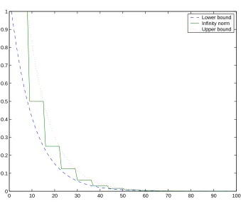
Lemma 2.1.3. SupposeGis weakly connected with a single vertex as the unique root strong component; for any given > 0, there exists a constant C such that
ρm( ¯A)≤ A¯m
∞ ≤
⎧⎪⎪ ⎪⎨
⎪⎪⎪⎩ 1C,·mρ<( ¯An)+m−n+1, m≥ n
(2.9)
for any positive integer m, where n is the order ofGandρ( ¯A) is the spectral radius of ¯A.
Proof According to Gerˇsgorin disk theorem [63], all eigenvalues of ¯Aare located in the unit disk, i.e.,
|λi| ≤1,∀i∈ {1,2,· · · ,n}.
Then,
ρ( ¯A)≤1=A¯ ∞.
Sinceρ( ¯Am)= ρm( ¯A), we have
ρm
Thus, the left half of inequality (2.9) is true. For the right half, we have
A¯m
∞ ≤ A¯ m∞ ≤1
according to the definition of the norm. So one is an upper bound. What we need to do next is look for a tighter upper bound.
If the graph is acyclic, there exists an indexing method so that ¯Ais a lower triangular matrix and all diagonal elements are zeros, i.e.,ρ( ¯A) = 0. Moreover, ¯An = 0 because the
length of the largest strong path is n−1. So we have
A¯m
∞ =0=ρm−n+1( ¯A)
if m≥ n. In other words, the infinity norm jumps from 1 to 0 when m increases from n−1 to n.
If the graph is not acyclic, any loop in the graph can generate path with infinite length. In any loop, there exists at least one vertex whose out-degree is bigger than 1 becauseG is weakly connected and the unique root strong component is a single vertex. Since every element in ¯Amis the gain of paths between certain pair of vertices with length m, all of the
gains converge to zero as m→ ∞, so
lim
m→∞
¯
Am =0. (2.10)
According to [101], it is true that equation (2.10) holds if and only if all eigenvalues of ¯A are inside the unit circle in the complex plane. Thus,ρ( ¯A)<1.
Since matrix ˆA = (ρ( ¯A)+ )−1A¯ has spectral radius strictly less than 1, ˆAm → 0 as
m → ∞ and the elements of sequence {Aˆm}should be bounded by a certain constant K. Then for m≥n, we get
A¯m
∞ = maxi
n
j=1|( ¯Am)i j|
≤ nKρ( ¯A)+m
≤ Cρ( ¯A)+m−n+1
0 10 20 30 40 50 60 70 80 90 100 0
0.1 0.2 0.3 0.4 0.5 0.6 0.7 0.8 0.9 1
[image:36.595.153.492.64.350.2]Lower bound Infinity norm Upper bound
Figure 2.4: Bounds of normalized adjacency matrix norm
Figure 2.4 shows an example of the bounds of ¯Aof a leader-follower formation with weakly connected topology. With properly chosen parameters, the upper bound given in Lemma 2.1.3 is much tighter than the upper bound 1.
2.2
Quantization and Distortion
A simple model of quantizer usually consists of two parts: encoder and decoder. The encoder has a set of partitions {V1,V2,· · · ,VM}, which are called quantization cells, over
the state space Rm. The number of cells M is countable. Also, V
i ∩Vj = ∅for any i, j ∈
{1,2,· · · ,M}with i j, and Ni=1Vi = Rm. For any x∈ Rmas the input, the output of the
encoder is an integer called the quantization index, which represents the quantization cell which x belongs to. So the encoder can be presented by a function as
The decoder has a codebook which defines a value ci ∈ Rm for every quantization index i,
i.e.,
r(i)= ci. (2.12)
The quantization rule of a quantizer is the composite function
r◦q(x)=ci = ˆx if x∈Vi (2.13)
where ˆx is the quantized representation of x.
Apparently, quantization is a lossy process since part of the data resolution will be lost. For example, for any x1, x2 ∈ Vi and x1 x2, we have r◦q(x1) = r◦q(x2) = ci.
Thus, a distortion function d(x, ˆx) : Rm× Rm → R+ is defined as a measure of the cost of
representing x by ˆx. One popular distortion function used for continuous state space is the
squared error distortion defined on a value-by-value basis as
d(x, ˆx)= (x− ˆx)2. (2.14)
If x is a random variable with the probability density function f (·) overRm, the average distortion is given by
E[d(x, ˆx)]=
Rm
d(x, ˆx) f (x)dx=
i
Vi
d(x, ˆx) f (x)dx. (2.15)
The bits per source sample (bpss) of a quantizer is the number of average binary bits used to transmit a quantization index from encoder to decoder. When a fixed-length coding scheme is used, the bpss equals to R=log2M. When a variable-length coding scheme is employed, the probability of each index i is pi =
Vi f (x)dx and the average bpss is given
by the entropy as
R=−
M
i=1
pilog2pi. (2.16)
A typical example of a variable-length code is the Huffman code [102].
Op-timizing a quantizer involves minimizing both of these. For a fixed-length coding scheme, optimizing performance reduces to minimizing quantizer distortion and two conditions must be satisfied [103]:
• The nearest neighbor condition. A source sample must be mapped to the closest ci;
• The centroid condition. The value of ci should be the centroid of cell Vi, i.e., the
expected value of the source sample given that it lies in the cell.
For a variable-rate coding scheme, the centroid condition is still necessary for the quantizer to be optimal.
Moreover, a quantizer is called a vector quantizer when m > 1 and is called a scalar quantizer when m = 1. The most popular quantizer is the uniform scalar quantizer where all cells are of equal size. The quantization rule of such a quantizer is characterized by three parameters: the size of its cells, which is often called the step size and denoted byΔ, the number of the cells, and an offset between zero andΔthat is used to locate partitions. The average distortion for uniform scalar quantizer with small step size is approximately Δ2/12.
2.3
Modeling for Packet Drops
For modern communication networks with high bit rates, packet drops can be caused by signal degradation over the medium (signal to noise ratio is too small), over-saturated network links (congestion in the network), faulty networking hardware, etc. A rich litera-ture about packet drops can be found and many mathematic models have been proposed. In this section, two popular models that are mathematically simple yet sophisticated enough to capture the characteristics of packet drops in large scale networks are presented.
are independent and identically distributed (i.i.d.). This model is characterized by a single parameterλthat has the probability ofγk being 1. So the model can be presented by
γk =⎧⎪⎪⎪⎨⎪⎪⎪⎩ 1 with probabilityλ 0 with probability 1−λ
(2.17)
Network
Good Bad
(b) (a)
Figure 2.5: Models of packet drops: (a) i.i.d. Bernoulli model; (b) two-state Markov chain model
Gilbert-Elliot Channel Model - Sometimes packet drops occur in bursts due to the memory effect of the network. This bursty error behavior can be represented by a discrete Markov chain. The simplest one is the Gilbert-Elliot channel model [96, 97], or the two-state Markov chain model, which is shown in Figure 2.5, part (b). In this model, the network jumps between two possible states: “good” and “bad.” In the good state, the packet is transferred successfully; while in the bad state, the packet is dropped. The current network state, Xk, depends only on the previous state Xk−1. Assuming that 1 means the good state and 0 means the bad state, the transition probabilities are
⎧⎪⎪⎪ ⎪⎪⎪⎪⎪ ⎪⎪⎪⎨ ⎪⎪⎪⎪⎪ ⎪⎪⎪⎪⎪ ⎪⎩
q01 = P[Xk = 0|Xk−1= 1]
q11 = 1−q01
q10 = P[Xk = 1|Xk−1= 0]
q00 = 1−q01
(2.18)
where qi jis the transition probability from the previous state j to the current state i. Thus,
the transition probability matrixQis given by
Q=
⎡ ⎢⎢⎢⎢⎢
⎢⎢⎢⎣ q00 q01
q10 q11
⎤ ⎥⎥⎥⎥⎥
Chapter 3
Double-Graph Control Strategy for
Formation Control
3.1
Formulation of Double-Graph Control Strategy
In this section, we formulate the problem of formation control for multi-agent systems and investigate the stability of the formation with respect to agent dynamics as well as the interaction topology.
3.1.1
Gain Matrix in Signal Flow Graphs
1
2
3
6
4
a
b
d
c
e
f
5
g
Figure 3.1: A signal flow graph
weight associated with each edge represents the gain by which the signal is multiplied when passing the edge. Using Mason’s gain formula, we can find out the actual gain from any input vertex to any output vertex. For multi-agent systems, we need to analyze all possible gains between any two vertices.
Let us start with a simple signal flow graph with six vertices as shown in Figure 3.1. Weights are listed along edges. By Mason’s gain formula, we get the gain from vertex 1 to vertex 6 as
g16=
abe+a f g
1−bcd .
The following lemma introduces a square gain matrix G = {gi j} where each element gi j
represents the gain from vertex vito vertex vj.
Lemma 3.1.1. For a signal flow graphG, the gain matrix is
G= (I− A)−1 (3.1)
whereAis the weighted adjacency matrix associated with the signal flow graph.
Proof With a little abuse of notation, we use Ai j to indicate the elements in A. It is
well known that elements in Am actually describe the sum of the gains of all paths with length m between any two vertices. For example,A23 = b indicates there is only one path
with length 1 between vertex 2 and 3 and the gain is b. A226 =be+ f g indicates there exist
two paths with length 2 between vertex 2 and 6 and the gains are be and f g.
If the signal flow graph doesn’t include any loops, thenAn = 0 since the longest pos-sible path has length n− 1. Otherwise, Ais not nilpotent. In Figure 3.1, the graph has a loop as 2 → 3 → 4 → 2. For the gain matrix G, it’s true that G6 0. For example, (1,2,3,4,2,3,4,2,3,6) is a path from vertex 1 to 6 with length 9 and path gain ab3c2d2e. Then, we write the gain matrix as
by listing the gains of all possible paths. Since
(I − A)·G = (I − A)·(I+A+A2+A3+· · ·)
= (I +A+A2+A3+· · ·)
−(A+A2+A3+· · ·)
= I,
we have
Q= (I− A)−1.
Thus, we easily get the weighted adjacency matrix of Figure 3.1 and the gain matrix as
A= ⎡ ⎢⎢⎢⎢⎢ ⎢⎢⎢⎢⎢ ⎢⎢⎢⎢⎢ ⎢⎢⎢⎢⎢ ⎢⎢⎢⎢⎢ ⎢⎢⎢⎢⎢ ⎢⎢⎢⎢⎢ ⎢⎢⎢⎢⎣
0 a 0 0 0 0
0 0 b 0 f 0
0 0 0 c 0 0 0 d 0 0 0 0 0 0 0 0 0 g 0 0 0 0 0 0
⎤ ⎥⎥⎥⎥⎥ ⎥⎥⎥⎥⎥ ⎥⎥⎥⎥⎥ ⎥⎥⎥⎥⎥ ⎥⎥⎥⎥⎥ ⎥⎥⎥⎥⎥ ⎥⎥⎥⎥⎥ ⎥⎥⎥⎥⎦ G = ⎡ ⎢⎢⎢⎢⎢ ⎢⎢⎢⎢⎢ ⎢⎢⎢⎢⎢ ⎢⎢⎢⎢⎢ ⎢⎢⎢⎢⎢ ⎢⎢⎢⎢⎢ ⎢⎢⎢⎢⎢ ⎢⎢⎢⎢⎣
1 1−abcd 1−abbcd 1−abcbcd 1−a fbcd abe1−+bcda f g 0 1−1bcd 1−bbcd 1−bcbcd 1−bcdf be1−+bcdf g 0 1−cdbcd 1−1bcd 1−cbcd 1cd f−bcd e1+−f gdcbcd 0 1−dbcd 1−bdbcd 1−1bcd 1−d fbcd bde1−+bcdf dg
0 0 0 0 1 g
0 0 0 0 0 1
⎤ ⎥⎥⎥⎥⎥ ⎥⎥⎥⎥⎥ ⎥⎥⎥⎥⎥ ⎥⎥⎥⎥⎥ ⎥⎥⎥⎥⎥ ⎥⎥⎥⎥⎥ ⎥⎥⎥⎥⎥ ⎥⎥⎥⎥⎦
by the lemma. When we consider a multi-agent system, we treat it as a MIMO system and it is natural to analyze the gain matrix, i.e., the transfer function matrix. Suppose the input signal at vertex vi is ui. The outputs for the graph can be represented by
⎡ ⎢⎢⎢⎢⎢ ⎢⎢⎢⎢⎢ ⎢⎢⎢⎢⎢ ⎢⎢⎢⎢⎢ ⎢⎢⎢⎣ y1 y2 ... yn ⎤ ⎥⎥⎥⎥⎥ ⎥⎥⎥⎥⎥ ⎥⎥⎥⎥⎥ ⎥⎥⎥⎥⎥ ⎥⎥⎥⎦
=GT ·
⎡ ⎢⎢⎢⎢⎢ ⎢⎢⎢⎢⎢ ⎢⎢⎢⎢⎢ ⎢⎢⎢⎢⎢ ⎢⎢⎢⎣ u1 u2 ... un ⎤ ⎥⎥⎥⎥⎥ ⎥⎥⎥⎥⎥ ⎥⎥⎥⎥⎥ ⎥⎥⎥⎥⎥ ⎥⎥⎥⎦ . (3.3)
This lemma requires that I − A is not singular. Otherwise, at least one element in G is unbounded and the signal gain from vi to vj is infinite. For a multi-agent system, that
3.1.2
Nyquist Criterion for Formation Stability
Suppose for a multi-agent system, there are n agents with identical linear dynamics denoted by
˙xi = Axi+Bui,
where i is the agent index. Each agent can get observations as
yi = C1xi
zi j = C2(xi−xj−Li j)
where j ∈ N(i) and Li j is the static offset based on the formation configuration. Based on
the signals yiand zi j, designing a local controller with identical structure for each agent is a
common distributed control strategy. A directed graphGis used to represent the interaction topology. Each vertex represents one agent. If agent i can get the state of agent j, then there exists an edge (vi,vj) inG. The directions of the edges are important. Usually, the errors
for relative state measurements are synthesized into a single signal ziwith equal weights as
zi =
1
dii
zi j, j∈ N(i)
where diiis the out-degree of vertex vi.
According to [99], a local controller stabilizes the whole formation if and only if it simultaneously stabilizes the following n subsystems:
˙x = Ax+Bu y = C1x
z = λi( ¯L)C2x
whereλi( ¯L) are the eigenvalues of the normalized Laplacian ¯L.
P(s). The transfer function for a single agent is
H(s)= P(s)C(s)
1+P(s)C(s). (3.4)
We can treat a multi-agent system as a signal flow graph with the inputs and outputs of each agent as signals. Figure 3.2 shows the interaction topology of a leader-follower multi-agent system where vertex 1 is the leader. The associated single flow graph is on the right side where yi is the output of agent i. In the signal flow graph, the weight associated
with edge (vi,vj) is H(s)/dj j. Please note that directions of edges are changed in order to
represent the directions of signals. It is easy to tell that the normalized adjacency matrices of these two graph are transposed, i.e., ¯Ainteraction =A¯ =A¯Tsignal.
Assuming that the input of agent 1 is signal u1(s). By Lemma 3.1.1, we get
⎡ ⎢⎢⎢⎢⎢ ⎢⎢⎢⎢⎢ ⎢⎢⎢⎢⎢ ⎢⎢⎢⎢⎢ ⎢⎢⎢⎣
y1(s)
y2(s)
...
yn(s) ⎤ ⎥⎥⎥⎥⎥ ⎥⎥⎥⎥⎥ ⎥⎥⎥⎥⎥ ⎥⎥⎥⎥⎥ ⎥⎥⎥⎦
= (I−H(s)·A¯Tsignal)−1·H(s)
⎡ ⎢⎢⎢⎢⎢ ⎢⎢⎢⎢⎢ ⎢⎢⎢⎢⎢ ⎢⎢⎢⎢⎢ ⎢⎢⎢⎣
u1(s) 0 ... 0 ⎤ ⎥⎥⎥⎥⎥ ⎥⎥⎥⎥⎥ ⎥⎥⎥⎥⎥ ⎥⎥⎥⎥⎥ ⎥⎥⎥⎦
= (I−H(s)·A¯)−1·H(s)
⎡ ⎢⎢⎢⎢⎢ ⎢⎢⎢⎢⎢ ⎢⎢⎢⎢⎢ ⎢⎢⎢⎢⎢ ⎢⎢⎢⎣
u1(s) 0 ... 0 ⎤ ⎥⎥⎥⎥⎥ ⎥⎥⎥⎥⎥ ⎥⎥⎥⎥⎥ ⎥⎥⎥⎥⎥ ⎥⎥⎥⎦ . (3.5)
In the general case, we have
⎡ ⎢⎢⎢⎢⎢ ⎢⎢⎢⎢⎢ ⎢⎢⎢⎢⎢ ⎢⎢⎢⎢⎢ ⎢⎢⎢⎣
y1(s)
y2(s)
...
yn(s) ⎤ ⎥⎥⎥⎥⎥ ⎥⎥⎥⎥⎥ ⎥⎥⎥⎥⎥ ⎥⎥⎥⎥⎥ ⎥⎥⎥⎦
=(I−H(s)·A¯)−1·H(s)
⎡ ⎢⎢⎢⎢⎢ ⎢⎢⎢⎢⎢ ⎢⎢⎢⎢⎢ ⎢⎢⎢⎢⎢ ⎢⎢⎢⎣
u1(s)
u2(s)
...
un(s) ⎤ ⎥⎥⎥⎥⎥ ⎥⎥⎥⎥⎥ ⎥⎥⎥⎥⎥ ⎥⎥⎥⎥⎥ ⎥⎥⎥⎦ . (3.6)
y2
y4
y5 y6
y7
y3 y1
Signal flow graph
H(s) H(s)
H(s)
H(s)
H(s)/2 H(s)/2
H(s)/2
H(s)/2 2
4
5 6
7
3 1
Interaction topology
Figure 3.2: Interaction topology and the corresponding signal flow graph
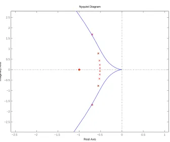
Lemma 3.1.2. The multi-agent system (3.6) is stable if and only if the net encirclement of
the critical points−(1−λi( ¯A))−1 by the Nyquist plot of P(s)C(s) is zero.
Proof We need the common denominator polynomial of the transfer function matrix to analyze the stability. According to the Schur decomposition theorem, there exists a unitary matrix T such that U = T−1A¯T is upper triangular with the eigenvalues of ¯Aalong the diagonal. The determinant of I−H(s)·A¯ is
det(I −H(s)·A¯) = detT ·(I−H(s)U)·T−1 = det(I−H(s)U)
= n
i=1(1−λi( ¯A)H(s)). Remember that the local closed-loop transfer function is
H(s)= P(s)C(s)
1+P(s)C(s),
then
det(I−H(s)·A¯) = ni=1 1+(1−λi( ¯A))P(s)C(s)
1+P(s)C(s) .
So the common denominator polynomial is
n
i=1
According to the Nyquist criterion, the critical point −1 is changed to n critical points
−(1−λi( ¯A))−1.
When G is strongly connected, 1 − λ( ¯A)i are the eigenvalues of ¯L and the lemma
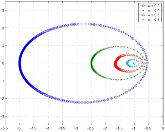
is consistent with the results in [99]. Distribution patterns of the critical points can be summarized as:
• Suppose z is a critical point, then Re(z)≤ −1/2. In other words, all the critical points are located on the left side of the axis of −1/2. This is a directed extension from Property 2.1.4.
• Since 1 is an eigenvalue of ¯A, then one of the critical points is at−∞. • IfGis symmetric, all critical points are real and no larger than−1/2.
• WhenGis complete, all critical points except−∞are located at−(n−1)/n
coinci-dentally.
Intuitively, loops inGintroduce periodic forces among agents and jeopardize the formation stability. The bigger these loops are, the more separated these critical points are, and the harder the design of the local controller is.
WhenGis weakly connected, the distribution patterns for the critical points are: • For any critical point z, it is still true that Re(z)≤ −1/2.
• According to Lemma 2.1.3, at least one eigenvalue of ¯Ais zero. So −1 is one of the critical points. Thus, stabilizing a single agent becomes a necessary condition for stabilizing the formation.
• IfGis acyclic, all critical points locate at−1 coincidentally since all eigenvalues of ¯A are 0. In that case, stabilizing a single agent is the necessary and sufficient condition for stabilizing the formation.
3.1.3
Double-Graph Control Strategy
is inspired by on-board sensing technology and eases the collision avoidance issue because, most likely, neighbors in interaction topology are consistent with those agents within short geometric distance.
One difficulty of this strategy is that the formation stability is sensitive to the interaction topology when agent dynamics is nontrivial. According to Lemma 3.1.2, when the interac-tion topology changes, local controllers may destabilize the formainterac-tion. A good example is given in [46] where an additional interaction link will destabilize the whole formation. In other words, we need to know the global knowledge of the interaction topology to design stabilizing local controllers. Another shortage is the poor disturbance resistance perfor-mance with respect to the size of the formation. Disturbance signals introduced at one agent can be magnified when they propagate to other coupled agents. That makes it im-practicable to maintain a larger size formation. This effect is noticed in acyclic topologies at first and numerous works have been written on how to bound this accumulation, such as the “string stability” problem in vehicle platoons [22, 23, 105] and the “mesh stability” for “look-ahead” systems in [25]. However, a uniform approach to obtain good disturbance resistance for arbitrary interaction topology and general agent dynamics is unclear.
Due to incredible developments in communication technology, the ratio of the cost to the communication bandwidth has dropped dramatically in the recent couple of decades. It is possible to equip each agent with communication devices at low cost. Then a com-munication network is formed and information can be passed around over it, which gives more flexibility and possibility to coordinated control for multi-agent systems. Based on this thought, we propose the double-graph control strategy as follows.
Suppose a coordinated multi-agent system has n identical agents. As shown in Figure 3.3, a directed graph G1 is employed to describe the global coordination topology that is used for global objective seeking and distribution. Suppose the global objective is Oglobal and the local copy of the global objective in agent i is Oi, then these local copies need to
be synchronized overG1, i.e., O1 = O2 = · · · = On = Oglobal. For formation control, static
The global coordination topology, G1, actually describes the topology of the commu-nication network over agents. Each agent can “talk” and “listen.” Every edge in G1 de-notes a communication link between two agents. When the global objective Oglobal is pre-established, the most direct way for synchronization is broadcasting Oglobal over G1. One typical situation is the leader-follower formation control where the reference of the leader is a good choice of Oglobal. On the other hand, if the global objective is not clear be-forehand, distributed collective protocols are used overG1 to achieve the synchronization without centralized data collection and processing. Consensus protocols in [59, 64, 66], for instance, can be used for seeking Oglobalas a “virtual” reference of the formation struc-ture. Currently, general approaches for collective protocol design and analysis attract many researchers.
2
4 3
5 6
7 1
2
4
5 6
3 2
4 3
5 6
7 7
1 1
G1 G2 Double−graph strategy
Figure 3.3: Double-graph control strategy for multi-agent systems
Based on the local interaction topology, G2, local controllers of the double-graph con-trol strategy have identical structure shown in Figure 3.4. The dynamics for each agent is
Yi(s) = H1(s)·Oi(s)+H2(s)·
j∈N(i)Yi j(s) (3.8)
where H1(s) and H2(s) are transfer functions, Oi(s) is the error signal based on the global
objective, and Yi j(s) is the outputs of agent i’s neighbors. In order to simplify the analysis,
we choose transfer functions as
⎧⎪⎪ ⎪⎨
⎪⎪⎪⎩ HH12(s)(s) == α(1·−H(s)α)/dii·H(s)
where diiis the out-degree of vertex i in graphG2and 0≤ α≤ 1. Thus,
Yi(s)= H(s) α
Oi(s)+
1−α
dii
j
Yi j(s) .
(3.10)
That me