A Hybrid Shortest Path Algorithm for IKEA Warehousing System

2017 2nd International Conference on Computational Modeling, Simulation and Applied Mathematics (CMSAM 2017) ISBN: 978-1-60595-499-8

A Hybrid Shortest Path Algorithm for IKEA Warehousing System

Si-yu TIAN and Yu XIA

Northeastern University, 360 Huntington Ave, Boston, MA, 02115, United States

Keywords: IKEA, Warehousing, Relational database, Graph theory, Shortest path algorithm, Greedy algorithm, Dijkstra algorithm.

Abstract. Shortest Path Algorithms can be utilized to find the shortest distance between one vertex to another in a graph for logistics applications. In IKEA warehouses, the efficiency is reduced when customers squander time repeating routes in picking up their desired furniture. The shortest path algorithm implemented in this paper is to be a proper means of demonstrating the most efficient route with restricted intermediate nodes for customers. Since the traditional shortest path algorithm presents random intermediate nodes along the shortest path from entrance to exit. We proposed a shortest path algorithm that is suited to this circumstance as we used Greedy Algorithm to divide the original problems into three, as well as Dijkstra algorithm for calculating the shortest distance between two nodes. The data required in the Dijkstra algorithm is stored in IKEA warehousing relational database which is designed in this paper for simulation.

Introduction

With the development of optimization in industrial engineering [1], shortest path algorithms are widely used in different areas [2]. In logistics industry, implementing shortest path method in operational research [3,4] is a common way to save energy and time in transporting goods between logistic parks. Since transportation is the most crucial part considered in logistics, applications developed by companies are more focused on optimizing long-distanced routes. However, there are two other parts of logistics other than transportation – processing and warehousing.

In present electronic information age, relational databases [5] are broadly applied to warehousing information storage for quicker, easier management. Warehousing information often involves with the information related to the warehouse management and inventory control [6]. This article combines the traditional shortest path method which concerns with the location of the product as well as the destination in warehousing facilities and the technology-based warehousing information to constitute a more efficiency and timesaving management system.

IKEA [7] is a perfect example. As people know, IKEA is a company that sells ready-to-assemble furniture, kitchen appliances and home accessories across nations [8]. The typical IKEA store has two levels, the upper level for demonstration, while the lower level for buying and pickup. The lower level is separated into two sections, a section for home accessories and kitchen appliances, and the other section for furniture pickup. Generally, customers need to visit the upper floor and take note of the product they would like to purchase, and then visit the lower floor picking up their desired furniture at the pickup section.

Disparate functionalities at different levels in IKEA store has distinguished IKEA from other traditional shopping centers. Though the furniture location is known to customers from in-store computers or IKEA app, the actual locations of products are not predictable, hence customers still need to plan routes for pickup. This could result in time wasted on finding and repeating routes, which, contradicts to what the contemporary society is pursing for – efficiency. Consequently, given all these peculiarities of IKEA stores, it is in necessity to save time for customers and focus on efficiency improvement [9].

To resolve above issues, establishing mimic IKEA warehousing databases as comprehensive as possible could provide the basis of adding shortest path algorithms to relational databases. Finding the best algorithm by testing out different algorithms and calculating each one’s time complexity could therefore enhance time and efficiency for customers.

The rest of the paper is organized as follows. In section 2 we design the IKEA warehousing database. Section 3 describes how to analyze finding the shortest path problem and how to implement the algorithm theoretically. In section 4 presents Implementation of shortest path algorithm while in section 5 the algorithm is tested on real cases. Section 6 analyzes the advantage and disadvantage of the algorithm. Section 7 discusses how to improve this algorithm in the future.

Database Design

In this Section, the mimic database of IKEA warehousing system is established due to the unavailability to the real database.

The Purpose of the Database

Since we have no access to the identical IKEA warehousing databases, a predictive yet succinct version of their warehousing relational databases [10] is utilized in this paper, in which it contains different categories of the warehousing information.

Establishing Database

The database constituted below is based on the MySQL workbench 6.3.

The Information Required. In the IKEA warehousing database system, eight different categories were taken into consideration – product, customer, wish list, transaction, employee, plan, alert and supplier information.

Firstly, customer information is considered. If customers possess IKEA family membership card, the databases should store customer information, such as names, account number, shipping and billing addresses. When customers are browsing IKEA websites or their official app, they would like to add their desired products into shopping carts. Hence “wish list” category is needed to store what the customers would love to purchase, and quantity of them. The next category is product information. This category contains the detail information of products, including price, dimension, location etc. Transaction information is also taken into consideration. The unique transaction number is created when customers pay successfully either online or in store, along with the information of what customers purchased and how many of them. The difference between transaction and wish list category is that the wish list category is what customers are willing to buy, which is variable, while the transaction is what happens when the payment is successful. The next is plan information. Plan information displays the shortest paths results for customers. There is also an area called alert information. The meaning of alert is when products or carts decrease to a certain amount, the system will automatically apprise people who take in charge of this issue and get replenishment and restock in a rapid way. Another category is called employee information, which stores personnel information related to the warehousing system, and may include both managers and staffs. The last piece of information remained is supplier information. This category stores what companies is supplying for IKEA products.

Setting up Tables and Relationships. This warehousing database contains 23 different tables. Each category mentioned in the last section has several tables. There is a new feature that manages cart. Sometimes customers could not find the cart or when the cart quantity is in short, a sensor would be necessary on a cart to control total number of the carts, and to make sure when customers need it, they could easily find it.

which results in the reduction of the product amount. If the product number or the cart number decrease to a certain amount, the cart organizer or the manager would be notified. The manager takes charge with different kinds of staffs, and contact with the supplier.

The relationship between different entities could be described as one – multiple, or one – one, zero – one.

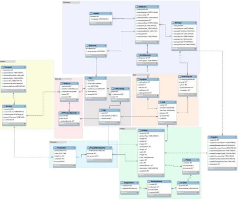
Product Category Details. In the product category, there are 4 tables created, which are called “Product”, “Pieces”, “Area”, “AreaStartEnd”, and “DistanceInfo” respectively. The detailed product like name, dimension, price information stored in the “Product” entity, in which the primary key is the unique product number. Due to the fact that one intact furniture may have one to multiple pieces for customers to pick up, “Pieces” entity stores the product ID with the corresponding components ID. The specific location information is stored in the “Location” entity. The primary key is the location number, which denotes the code number for a specific location of a product, and the specific location is called location Name. For example, area number 1 for a specific location Rack 24 Bin 23. The distance between each product and all the other products are stored in “DistanceInfo” entity. The distance from node 1 to node 2 is considered as same as that of 2 to 1. Distance Id is stored in distance info entity. This entity stores the distance between two nodes. “RouteStartEnd” entity stores the route information of the starting point and the end ending point. For instance, routeId 111 represents route starting from point 1 to ending point 2, while distance 112 represents route starting from point 2 to point 1, although they have same distanceId.

The comprehensive Entity Relationship Diagram(ERD) shows in Figure 1.

Shortest Path Algorithm Description

Terminology Definition

Dominator: Dominators are the nodes a customer must pass by, including the product they would like to pick up, and the starting node (entrance) as well as the ending node (exit). Free Node: Free nodes are nodes where customers may possibly pass by other than those dominators in order to get the shortest path results. Product List Dominator: These are dominators without the starting node or the ending node. Local optimum (aggregate): Divide the whole problem into small pieces, which are called subproblems. If the optimal solution is exited and could be computed in the subproblem, this solution is the local optimum solution. Local optimum aggregate is occurred when multiple local optimums in existence. Global optimum (aggregate): Every local optimum in each subproblem comprises the global optimum for the original problem. If there are multiple global optimums, these are called global optimum aggregate.

Problem Description

Each customer starts off from the starting node, ended in the ending node and they must go to at least one dominator to get their desired products. In order to pick up products, other than dominators, customers could possibly pass zero to multiple free nodes. Based on the above two facts, the problem of this paper is to calculate the shortest path, including dominators and free nodes in order to get the optimal result.

Algorithm Development Introduction

Greedy algorithm [11] is a solution of finding a global optimum by making local optimal choice at every stage.

Shortest Path Algorithm Implementation

The process of pre-processing the shortest path result and the distance result is in Section 4.1. Section 4.2 states how to get the shortest path result according to according to Section 4.1 based on the user input.

If a complicated problem could be solved by dividing the original problem into subproblems, moreover, if the global optimal solution could be found out using local optimal solutions by recursive method, which means global optimum could be deduced by local optimums, then greedy algorithm is an effective method to solve these problems.

According to the greedy algorithm, if every subproblem has an optimum, the final solution to the original problem could be viewed as optimal or nearly optimal.

In this specific question, the problem could be divided into 3 subproblems. Each subproblem has its own local optimum while the global optimum or the acceptable global optimum is summing up each local optimum.

Subproblem 1 is the distance between dominators. Subproblem 2 is the distance from starting node to the first dominator. Subproblem 3 is the distance from the last dominator to the ending node.

Let Ventrance denotes entrance while Vexit represents exit, and V1, V2, …, Vn represents each dominator. minDist() stands for the shortest distance composed of at least 2 nodes. Do permutations for the array of all dominators, and calculate the following 3 parts.

Part 1. Assume V1 is the first element of every permutation, and Vn denotes the last one. This set of permutation could be expressed as V1, V2, V3, …, Vn, and its shortest path is minDist(V1, V2, V3, …, Vn). The current shortest distance totalMinDistance = minDist(V1, V2, V3, …, Vn).

Part 3. Add the result of part 2 to the shortest distance from Vn to exit. The distance between Vn to exit is expressed as minDist(Vn, Vexit). The current shortest distance changes to totalMinDistance = minDist(V1, V2,…, Vn) + minDist(Ventrance, V1) + minDist(Vn, Vexit).

When the above three parts are completed, choose the array of dominators that has the minimum totalMinDistance.

Data Preliminary

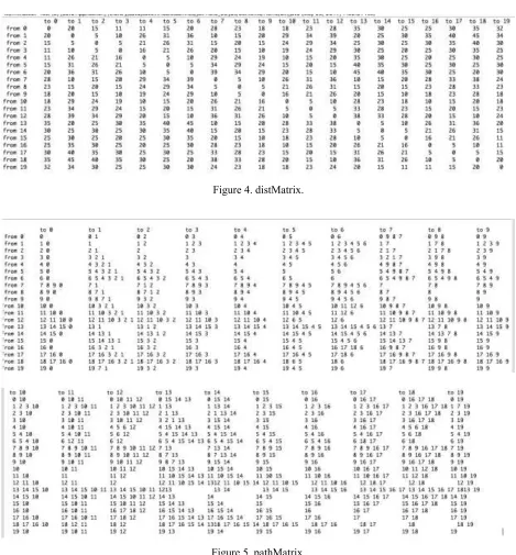
There are three steps happened in this section using Dijkstra Algorithm [12,13]. Step 1 is to store the node information extracted from warehousing database in an adjacency matrix called distMatrix. Step 2 is to use DFS (Depth First Research) [14] to iterate over all nodes from the starting node to see if there is any node that could not be reached. Step 3 is that if there is any node that could not be reached, delete the node, and then update the adjacency matrix. Step 4 it to calculate the distance between every two nodes with Dijkstra algorithm method [15], and renew the previous adjacency matrix with the newest shortest path length this algorithm displays. Save the path with shortest path into another matrix which is called pathMatrix.

function Dijkstra(Graph, source, destination): create vertex set Q

create array dist[] to store the min distance from source to each vertex create array prev[] to store the last vertex iterated

for each vertex v in Graph: //Initialization dist[v] ← +∞

prev[v] ← null add v to Q

dist[source] ← 0 //the distance from source to source is 0

while Q is not empty:

u ← vertex in Q which has the min dist[u] //Find the nearest vertex remove u from Q

for each neighbor v of u alt ← dist[u] + length(u, v)

if alt < dist[v] dist[v] ← alt prev[v] ← u

return dist[], prev[]

dist[destination] will be the shortest path length from source to destination. The shortest path can be got by prev[] in the nest step. Secondly, get the shortest path with Dijkstra Algorithm.

function getShortestPathByDijkstra(prev)

create new array shortestPath[]

foreach i from 0 to prev.length – 1

shortestPath[i] = prev[prev.length – 1 - i]

return shortestPath[]

Shortest Path Calculating Algorithm for IKEA Warehousing

The input of this algorithm is the array of all dominators, while the output is the sorted string consisting of all dominators with/without free nodes.

appeared dominator and exit. The resulting distance, which is called alternative distance, is the sum of the three distances mentioned above. If this alternative is shorter than the present global optimum, set this alternative as the new global optimum. Step 5 is based on the pathMatrix, to show free nodes, if there is. Step 6 is to output the sorted route result, which includes dominators and free nodes that a customer needs to pass by.

Function getShortestPath(distMatrix, pathMatrix, dominatorList)

n ← the amount of dominators

//get all permutation of dominators

List(V1, V2 … Vn) ← permutate(domonators) totalDistance ← 0

shortestPath ← null;

for each (V1, V2, … Vn) in List

currDistance ← 0;

for each i from 1 to n – 1

currDistance ← currDistance + distMatrix[Vi][Vi+1];

currDistance ← currDistance + distMatrix[0][V1];

currDistance ← currDistance + distMatrix[Vn][distMatrix.length - 1];

if currDistance < totalDistance totalDistance ← currDistance

shortestPath ← this(V1, V2… Vn)

find the shortestPath with free nodes by pathMatrix;

return shortestPath

Algorithm Analysis

Let n be the total number of all nodes. Let m be the total number of dominators.

Time Complexity Analysis on Pre-processing Step. In the pre-processing step, shortest path is calculated through Dijkstra Algorithm from each node to every other node. The time complexity of calculating the distance from n nodes to every other node is O(n * n2), given the known time complexity of Dijkstra is O(n2). The pre-processing step takes enormous time, for a relatively complex, large-scaled map. However, this algorithm is designed for IKEA warehousing system, whose map is not unpredictable or complicated, also, the shortest path and the distance could be stored in memory in Matrix format with time complexity of O(n2). Therefore, this algorithm can be implemented on IKEA warehousing system.

Complexity Analysis on Shortest Path Algorithm for IKEA. The time complexity is O(m2) when doing permutations for the array of nodes. After the permutation step, the time complexity would be at least O(m*m!) when operating the process of finding the shortest path. Therefore, this algorithm, is unable to bear too many dominators as the system cannot sustain the volume.

In conclusion, high time complexity is only occurred when the first time running the preprocessing process, while in the following operations, there is no need to calculate what the shortest path is and the shortest path distance will be because these pieces of information are already stored in memory. Therefore, this algorithm is appropriate for implementing on IKEA warehousing system. In addition, this method does not require double counting the shortest path. It only requires implementing pre-processing process once when products are ready on the shelf.

Experimental Simulation

Experimental Environment

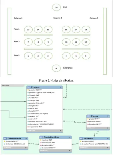
These 1-18 nodes locate on the aisle between two shelves. In other words, between two shelves which are represented in Figure 2 by rectangle shown below is a row of nodes.

18 nodes are divided into 2 sides which makes each side has 9 nodes. The reason that 9 nodes are chosen on each side is 3*3 nodes are the simplest case that could demonstrate the situation that contains row 1 and row 3, instead of the situation only contains two adjacent rows. Figure 2 shows the demonstration of how products displayed in IKEA warehouse.

Figure 2. Nodes distribution.

Figure 3. Routing information in database.

Data Extraction. Node data is extracted from IKEA warehousing database shown in Figure 3.

In order to simulate the purchase situation, first we start with product ID, then find the component location of a product and the distance between different components.

After pre-processing, there are two matrices than can be acquired. Figure 4 and Figure 5 shows the Matrices after pre-processing step.

Figure 4. distMatrix.

Figure 5. pathMatrix.

Testing Situations

The testing situation that may occur in reality describes below. The node data is from warehousing database.

Customer not Inputting Anything. This situation happens when customers don’t buy anything

as they go straight from entrance to exit. In this situation, this shortest path application can only be initiated if customers input product ID. If they do not do as required, the system will ask them to reenter product ID.

Customers Buying Product Extremely Far away from Each Other. For example, one customers would like to pick up from node 1,18,7,12,13,6. The Test set is {1,18,7,12,13,6}. Figure 6 shows the result.

Figure 6. Result of test in situation 5.2.3.

This algorithm runs perfectly smooth under this circumstance. Based on this result, it could be concluded that the time this algorithm consumed is merely concerned with product quantity as it does not relate to the node distribution. Therefore, this algorithm applies great to the building structure that has fixed number of shelves but with complex routes, like IKEA warehouse.

Customers Adding Repeated Products. Customers can only add the same product once. If they do not, the system will ask customers to reenter the data. Once the data is accepted, the system will begin to calculate the shortest path for customers.

Algorithm Analysis

It is proved that, according to the operation results, when node quantity is less than 10, this algorithm could completely satisfy customers’ needs. There is no obvious waiting time since limited quantity of nodes is tested. Further testing is required using graphs containing more nodes.

Results

From algorithm perspective, this algorithm meets the needs of finding the shortest path for customers. Yet further optimizations can be made to improve pre-processing steps, for example, implementing Dijkstra algorithm based on Fibonacci Heap method. After optimizing this, more complicated maps with a large number of nodes could be processed.

The algorithm of finding shortest path in this paper is suited to dense graph, which means high-density routes that consisted of various nodes. The reason for this is that time complexity of Dijkstra Algorithm in pre-processing step, as well as of permutation method for dominators, are concerned only with Vertices quantity, not edges quantity in graph.

This algorithm is also suitable for calculating shortest path multiple times for the same graph. This is because the pre-processing step only happens once after managers storing product location information into the system. Once this step is completed, calculating becomes easy because the system will search the required information in the system when customers input the product ID.

However, there are still some disadvantages of this algorithm. This algorithm cannot support too many nodes as it requires permutations for every dominator. For instance, if there are 11 nodes, the permutation would be 11! = 39916800, which means the final result is shown after 39916800 times of calculation. As a result, the algorithm runs slow and this would impact user experience.

Further optimization of this algorithm on pre-processing step, such as implementing Dijkstra Algorithm using Fibonacci Heap, could improve calculation efficiency for the graph that contains too many nodes.

Discussion

In practice, this algorithm is not limited to finding the shortest path for IKEA. It can also be applied to similar problems on path planning as long as they contain must-pass nodes, like delivery problems [17], and tour route planning problems.

The graph used in this paper is weighted undirected graph, however, this algorithm can also be applied to weighted directed graph which does not need to be modified. For unweighted undirected or directed graph, if two nodes are connected, it only requires to change weights to 1 in distMatrix() in pre-processing step, or if two nodes cannot be connected, change weights to +∞.

The biggest limitation of this algorithm is that it is not able to deal with large quantity of nodes. If there are too many nodes input in the system by customers, customers need to wait a long time for results to come out as the operation efficiency is dramatically decreased. Further optimization is needed to find other ways instead of permutation, for example, always finding the nearest dominator to the customer, to get the result, in order to satisfy the needs of inputting more nodes. But for IKEA warehousing area of no great size, there are not too many nodes a customer would like to choose. Hence it could be concluded that this algorithm meets requirements.

At this stage, this shortest path result, which is currently stored in memory, implemented by extracting data from databases and running the algorithm on JAVA platform, instead of storing the shortest path result back into the database. Additionally, further optimization on integration of the IKEA official App [18] and this shortest path algorithm could facilitate customers to save their time by visualizing shortest routes after customers adding products into shopping list.

Reference

[1] Godfrey C. Onwubolu, B. V. Babu, New Optimization Techniques in Engineering, 2004.

[2] Maurizio Bruglieri, Alberto Colorni, Federico Lia, Alessandro Luè, A multi-objective time-dependent route planner: a real world application to Milano city, 2014.

[3] Rommert Dekkera, Jacqueline Bloemhof, Ioannis Mallidisc, Operations Research for Green Logistics – An Overview of Aspects, Issues, Contributions and Challenges, 2011.

[4] D. Ghosh, Logistics Cost Minimization, An approach with Operations Research Models, 2015.

[5] E.F. Codd, The relational model for database management: version 2, Addison Wesley Publishing Company, Boston, 2000, Chapter 1 “Introduction to Version 2 of the Relational Model”.

[6] Alex Scotti, Mark Hannum, Michael Ponomarenko, Dorin Hogea, Akshat Sikarwar, Mohit Khullar, Adi Zaimi, James Leddy, Rivers Zhang, Fabio Angius, Lingzhi Deng, Comdb2 Bloomberg’s Highly Available Relational Database System, 2016.

[7] Ikea official website http://www.ikea.com/us/en/

[8] IKEAWorldMap - Inter IKEA Systems BV. http://franchisor.ikea.com/worldmap/interactive.html

[9] Willian Applebaum, Studying Customer Behavior in Retail Store Journal of Marketing, Vol. 16, No. 2 pp. 172-178, 1951.

[10] Best Practices Maksym Petrenko, Amyris Rada, Garrett Fitzsimons, Enda McCallig, Calisto Zuzarte, Physical database design for data warehouse environments, 2012.

[11] Cormen, Leiserson, Rivest, Stein, Introduction to Algorithms, 2001, Chapter 16 "Greedy Algorithms".

[13] Cormen, Leiserson, Rivest, Stein, Introduction to Algorithms, 2001, "Chapter 24 Single-Source Shortest Paths 24.3 Dijkstra’s algorithm".

[14] Wikipedia: Depth-first search(DFS) algorithm.

[15] Wikipedia: Dijkstra algorithm.

[16] Youssef Bassil, A Comparative Study on the Performance of Permutation Algorithms, Journal of Computer Science & Research (JCSCR) - ISSN 2227-328X. http://www.jcscr.com Vol. 1, No. 1, Pages. 7-19, February 2012.

[17] Krusralji, J. B, On the Shortest Spanning Subtree of a Graph and the Travelling Salesman Problem. proc. Lmer. Math. Soc. j, 48_S; (956).