MODELING LINK FOR OCEAN WAVE ENERGY OF POINT ABSORBERS: A MATHEMATICAL FRAMEWORK

MODELING LINK FOR OCEAN WAVE ENERGY OF

POINT ABSORBERS: A MATHEMATICAL

FRAMEWORK

Lorenzo Baños Hernandez1,†,‡

1 _{SIANI, Edificio Central del Parque Cientifico y Tecnologico, Campus Universitario de Tafira, 35017 Las}

Palmas de Gran Canaria (Spain)

* Correspondence: [email protected]; Tel.: +34-661-341-683 † The author declares full ownership of the presented divulgation.

Abstract:This compendium presents new mathematical techniques for modeling Point Absorbers. A combined frequency-time domain framework is developed. It is used to simulate the energy generated by the wave farms. With Matlab and Fortran as a base, this leads to obtain physical variables of primary importance, namely position, velocity and power to energy net balance relationships of absorption. Integration of different degrees of freedom with heave as main executable leads in turn to a single buoy motion focus. Acquisition of the needed hydrodynamic coefficients is provided through application of potential field solvers with Boundary Element Methodology background. Initially, this Wave-to-motion model is validated by comparison with previous experimental results for a floating cone cylinder shape (Buldra-FO3). A single, generic, vertical floating cylinder is contemplated then, that responds to the action of the passing regular waves excitation. Later, two equally sized vertical floating cylinders aligned with the incident wave direction are modeled for a variable distance between the bodies. For both unidirectional regular and irregular waves as an input in deep water, we approximate the convolutive radiation force function term through the Prony method. By changing the spatial disposition of the axisymmetric buoys, using for instance triangular or rectangular shaped arrays of three and four bodies respectively, the study delves into motion characteristics for regular waves. The results highlight efficient layouts for maximizing the energy production whilst providing important insights into their performance, revealing displacement amplification- and capture width-ratios, while deriving in possible interpretations of scenarios related to the known park effect. These terms are encompassed by the novelty of a new conceptual Post-Processing methodology in the field, which leads to obtain an optimal distance for the separated bodies with effective energy absorption in a regular wave regime. The main objective is to generate a tendency within the hydrodynamic field of study, which is the Wave to motion perspective. More generally, this computational excursion envisions and depicts potential fields of study, which will surely enhance new connections and link this renewable energy form. Therefore, this research delves first into the historical and technical background on Ocean Wave Energy. Next, it is in the section regarding Materials and Methods, where boundaries and related equations are introduced step by step, together with latter mentioned case scenarios, and their corresponding configuration parameters. A separate section frames then the scope of results, while finally, there is an ensuing discussion and conclusions for evaluation assessment.

Keywords: Ocean Wave Energy; Fluid-Structure Interaction; BEM; Diffraction/ Radiation; Floating Cylinder; Heave; Array

1. Introduction

Among the large list of patented Ocean Wave Energy Converter (WEC) types, the Point Absorber (PA) technology has become predominant in the field according to [1]. Studied intensively since the

Table 1.Research roadmap for the numerical approach Regular waves regime

Procedural Steps Focus Objective Case scenario

A Data handling Numerical (BEM) and Testing results acquisition 1 buoy

B Time-frequency Domain model Hydrodynamics 1... ->... 2 buoys

C Post-Processing Visualization and Experimental comparative 1... ->... 3 buoys

D Assessment Evaluation 1... ->... 4 buoys

E Optimization fronts on a B-D base 1... ->... 4 buoys

oil crisis during the late 1970’s by Budal and Falnes [2] in Scandinavia and by Evans [3] in parallel in the United Kingdom, focus was set upon the Mathematical & Physical Modeling of such devices among others. They are best described by the fact that their characteristic length is much smaller than the surrounding wavelength from the passing waves. Nowadays, several countries all over the world are investigating the performance of this technology [4]. PA’s can be floating or bottom-mounted structures, with a Power-Take-Off (PTO) mechanism. They vary depending on the oscillation mode of the geometry. Most of the devices use mainly the vertical displacement (heave) of the structure induced by the incident waves to activate the electricity generation either through hydraulics or directly using magneto-inductive components. By positioning and connecting several units close to each other, the system is addressed as a multipoint absorber [5]. Another possibility is to deploy lines or "matrices" of single PA’s in order to cover a larger area, while absorbing more energy. These so-called Arrays might become the future of Ocean Wave Energy, since they not only produce more energy in theory, but they can also be adapted to existing floating structures, such as Floating Production Storage and Offloading vessels [7] or offshore wind energy foundations. Similarly to the way pump storage plants alternate energy production between turbomachinery and wind turbines [8], WEC’s might supply Wind Energy during its production flaws, since it is a much more constant resource [9]. The State of the Art of the modeling procedure for this work is schematized next:

In Table1it is noted, that the step-by-step table has been determined with specific focus on previous project experience in the field [10]. Procedure steps A-E involve a pre- / solver / post-processing structure, that ranges from 1−4 point absorbers. It also includes certain optimization perspectives at the end stage E as a feedback loop, which might in turn lead to restart at A again.

A deeper look in Europe at some implemented projects (incl. real sea testing) reflects the following list

Wedge Global buoy (Gran Canaria-Spain)

Pipo Systems buoy (Gran Canaria-Spain)

OPT buoy array (Spain)

Searev (France)

Tecnalia-BIMEP point absorber (Basque country-Spain)

Corpower buoy (Sweden)

Seabased buoy (Sweden)

ISWEC (Italy) AWEC (USA)

At multipoint absorber level, two main projects are highlighted, namely:

Wave Star Energy (Denmark-Europe)

Albatern WaveNET (Scotland-Europe)

Emphasis is set upon the insular base, which surrounds the Canary Islands, due to

• location-based proximity: either european or outer borders

• proven concept: based on prototype technical reports

The first seven projects correspond to single Point Absorbers, while the two remaining products represent Multipoint Absorbers. From the total number of introduced projects, only two are being tested right now, namely the Wave Star and WaveNET. For a broader perspective on latter mechanisms, further global documentation can be found in [1].

However, certain drawbacks have to be considered before deploying such converters in the sea. The first issue corresponds to the high corrosive, harsh environment, which is the ocean. Then, there is the need for large infrastructures, such as mooring lines, both to anchor the floater to the bottom and to transmit the electricity to shore if the PTO is in the PA itself. Also, there is always a risk of encountering extreme wave conditions, which may affect the device during operation. All of these arguments determine the importance of minimizing costs during design and test phases, while considering possible worst case scenarios. Computational methods employed during the course of this research are a consistent approach to achieve the mentioned purposes, specially with respect to hydrodynamics.

The number of different applied numerical methods in Ocean Wave Energy is increasing steadily [11]. Since it is also noted, that computational capacities are growing exponentially [12], it is a matter of time before the scientists will be able to describe real fluid phenomena with certain accuracy. For the given cases, a combined BEM-frequency-time domain analysis will take place. For a so called wave to wire (W2W) model [13], this means, that first, hydrodynamics coefficients are determined for the wetted geometry. Next, these parameters are attached to the equations of motion in the model solver, which in turn generates amplitudes of oscillation, velocities and power (energy) absorbed by the PA’s in either frequency domain or time domain. In short, given an input wave incidence, the codes compute pressure and velocities on the panels (FEM), and determine characteristic hydrodynamic parameters. Latter ones can be employed to solve the governing equations of motion, which in turn, depending on the chosen domain (either time or frequency), will provide insights on the motion displacement patterns.

As in any other related field, optimization is the keyword to refine the overall performance of the technology. From the hydrodynamic point of view, there are mainly three arguments that have to be taken into account in order to obtain maximum energy. The first one refers to the oscillation mode of the device. [14] determined that combining heave and surge, the device will absorb more than 80% of the available Wave Energy. Hence, one has to find suitable geometries and PTO systems that can superpose the different degrees of freedom. The geometry itself turns out to be determinant, and thus becomes the second argument. The Salter’s duck is the only patented device mechanism, that is theoretically nearly capable of absorbing all the incident wave potential [15,16]. Last but not least, near-resonance conditions have to be determined for achieving a narrow operational bandwidth of the PA [17], from which to obtain its maximum amplitude motion.

2. Materials and Methods

Throughout the course of this research, certain conditions have been met for the incoming waves and more specifically for the floating systems. This involves choosing the correct physical and mathematical background for the underlying theory behind. Both subjects are treated in the following section.

2.1. Assumptions

According to the wave mechanics theory, following characteristics are being considered:

• Linear Potential Airy theory

• Various Depths (ranges from shallow water to deep water)

• Unidirectional regular and/or irregular waves (specified on own Phd thesis)

Regarding the floating system, further limitations are introduced next:

• Mooring, viscous and damping forces have been determined empirically, using previous thesis results from Bosma [20].

• The PTO force is estimated randomly for the generic heaving cylinder, since no such an existing physical device has been found with published damping characteristics.

It is noted, that basically, unidirectional regular waves are used as an input to the model, as stated in1. Irregular superpositions are only mentioned due to the own PhD thesis carried out by the author. Linear potential or so called Airy theory applies to the previous mentioned sea states, mainly based on small amplitude wave heightsHwith ratios such that _DH

h << 1 corresponding to shallow water and H

L << 1 referring to deep water. Here,Dh represents the water depth, andLis the wave length. For the boundaries, classical periodicity and Sommerfeld radiation appear at inlet and outlet respectively. Thereby, the open-source Diffraction-Radiation solver NEMOH (BEM) is used for the acquisition of the hydrodynamic coefficients in the frequency domain. These are added mass (Ar), radiation damping (Ch) and excitation force (Fe) as sum of diffraction (Fd) and Froude-Krylov forces (Ff k). Additionally, one obtains in the time domain the values for Ar at ω → ∞ and Impulse Response Functions for

the radiation force functionkr(t)(retardation kernel). All these terms become part in the solution of Newton’s equations of motion, whereas specific terms have to be first integrated in convolutive form, for instance the radiation forceFr.

2.2. Hydrodynamic Equations of Motion

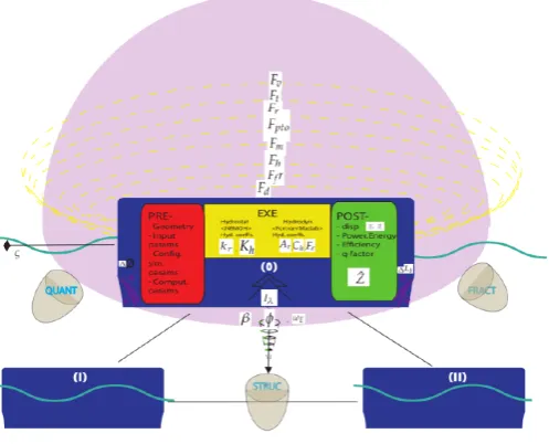
Figure 1.Fluid-Structure Interaction: Current modeling scheme and future envisioning strategy

Taken the PA system as a whole software application itself, one does not only provide fundamental simulation theory and the main focus of this work (navy blue rounded shape (0)) related to the present investigation, but it also envisions future perspectives (yellow dashed ellipsoids), while foreseeing new research fields (grey nodal shapes). It is merely an abstraction of a black-box system, which includes systematically further optimization strategies (confer to violet variable NACA profiles on the bottom corners of (0) in Figure 1. Assuming (0) as the starting unit confronting the waves, the scheme is extended hereby into a small triangular array (objects I and II), which is expected to perform efficiently. Moreover, from the base to the top of the sketch,1reflects the hydrodynamic entry with wave amplitude

ζ(in turquoise), including the most relevant parametric units. In the middle part, the structure presents

the classical vibration and computational approach. Reaching the top, the spreading ellipsoidal dashed curves represent characteristic force vectors, which might be tuned in advance for whatever focus research tendencies might converge into.

From the main "EXE" workflow, one can first deduce, how the hydrostatic and hydrodynamic parts are introduced by the BEM calculation. In the middle part, a modified Mass-Spring-Damper (MSD) equation is solved, which is a second order ordinary differential equation in the form Mtz¨ = ∑F , whereasMtinvolves the total mass of the floating body. Additionally, simple (double) dotted variables denote first (second) order time derivatives of position, velocity and position respectively. In this case, the z formulation refers to the heave component in vertical cartesian coordinates. Moreover, this procedure assumes that the surrounding water medium can be replaced by multiple spring and stiffness coefficients, which are then inserted into the discretized equation. Furthermore, the sum of forces becomes∑F = Fe+Fr+Fh+Fm+Fpto, from which one can assume the single components information. First item on the RHS is the excitation force, which can be formulated through the following convolution integral

Fe=

Z ∞

−∞fe(t−τ)η(τ)dτ, (1)

whereτrepresents the causality time span, such that some previous stage is taken out of memory

in advance. Second term is the radiative term, which is described generally by the equation

Fr =−Ar,∞−

Z t

with ˙zas the vertically displacing velocity component of the radiating body in motion. The third term inserts the hydrostatic restoring vector into the sum of forces, yielding

Fh=−Khz, (3)

with Khas the hydrodynamic stiffness. Fourth term considers the application of a mooring force on the floating system, such that

Fm=−Kmz, (4)

where Km stands for the mooring coefficient. Last term includes the PTO-force, which is simply reflected as a damping mechanism in the form

Fpto =−CPTOz,˙ (5)

whereas CPTO represents the PTO damping coefficient. There is the spectral distribution S(ω),

which serves as the last input to the model. One can calculate out the free surface elevationη, which

is then convoluted with the diffraction forceFd to determine the heave excitation force. It is noted at this stage, that a simple equation form for the excitation force in regular waves has been considered for this research according to [24–26], namelyFe(t) =Aw|Fe(ωE)|cos(ωEt+φ+∠Fe). Here,Awrepresents the wave amplitude, while|Fe(ωE)| is the computed magnitude of the diffractive force term for the excitation frequency ωE and both φ and ∠Fe correspond to wave phase shift of initial free surface elevation state and exciting angle respectively.

For multiple bodies, the equations of motion are introduced explicitly for the sake of clarity with respect to the two-body system as follows

Z1=

Fe1ηˆ+ω2₋ A12Fe2ηˆ

ω2(M2+A22)+iω(C2+C22)+Kh2

−

iω₋ C12Fe2ηˆ

ω2(M2+A22)+iω(C2+C22)+Kh2

(6)

Z2= Fe2ηˆ+Z1(ω 2_A

21−iωC21) −ω2(M2+A22) +iω(C2+C22) +Kh2

, (7)

Hereby, each variable is divided by ς = ηˆ, whereas the denominator term

corresponds to −ω2

n

(M1+M11) + A12

−ω2(M2+A22)+iω(C2+C22)+Kh2(ω

2_{A21−iωC21)}o ₊ iω

n

(C1+C11) +_−ω2_(M2+A22)+C12_{iω(C2+C22)+K} h2(ω

2_A

21−iωC21)

o

+Kh1.

With regard to the radiation force determination, different alternatives have been used up to date in order to approximate the integral. The common approach is to use a rational function fit, such as done by [27–29]. Another very efficient procedure turns out to be a digital filtering technique named the Prony’s method [30,31], which is implemented in this case for an exponential function approximation of the convolution integrals of radiation.

Once the different coefficients have been determined and loaded into the program, the program finds solutions for displacement, velocities and accelerations both in time domain and frequency domain for a given initial value problem of position and velocity. For the 2nd order partial differential equation in the adapted MSD form, one calculates iteratively the integrals of acceleration and velocity through an order reduction in the time domain. Integration methods need to be applied in order to be able to solve the derivatives. Following the state-of-the-art in numerical modeling of WEC’s [11], both a classical explicit Runge-Kutta method of 4th order (RK4) and an implicit Newmark Generalized-α

method (Nm-gen-α) have been implemented during the conducted research. First one presents an

βG and γG are numerical parameters that control both the stability of the method and the amount of numerical damping introduced into the system by the method [52]. ForγG = 1₂ there is no numerical damping; forγG >= 1₂ numerical damping is introduced. For this study in particular, when solving the equations of motion for more than one floating body, two additional matrix inversion methods have been used in Matlab. They are needed when solving the acceleration terms for accessing the Equation of Motion (2.2). Method 1 inverts the total massMt= M+Ar,∞term and leads to ¨z= M−t1(∑F). Then, one only needs to integrate the acceleration twice to get the remaining variables. In the second method, the mathematically considered coefficient matrix Abecomes much more dense, since it does not only include the total mass, but it also incorporates PTO damping and hydrodynamic stiffness. This way, the equation leads to the generalized formX= A−1b, whereas e.g. the state vector becomes in a single degree of freedom the formX= [z¨1, ˙z1,z1, ..., ¨zi, ˙zi,zi]Tandb= [Fe,1−Fr,1, ˙z1,z1, ...,Fe,i−Fr,i, ˙zi,zi]T. On the RHS, initial values are being inserted forz1, ˙z1, ...,zi, ˙zi. Then the model calculates the force absorbed and so determines the b vector. Now, it is straightforward to make the inversion of theAmatrix [k x k] on the left hand side for obtainingz, ˙zand ¨zthe same way it worked for the previous Mass-Matrix Inversion method. It leads to exactly the same analytic result as method 1, but its matrix formulation can become rather cumbersome depending on the i,j combination.

For the frequency domain, the Response Amplitude Operator (RAO) represents the magnitude of the displacement ˆZdivided by the incoming wave amplitudeςas a function of frequency. For one body

with a linear PTO damper as an example, the equation yields

ˆ Z

ς =

Fˆe(ω)

−ω2(M+Ar∞) +iω(CPTO+C_h(ω)) +K_h (8)

Remark is set upon the fact, that analytically, the research has made it possible to determine as well the RAO for two interacting bodies. For this reason, the approach is addressed as an alternating frequency-time domain model, where

Having introduced the main hydrodynamic variables and numerical schemes, it is worth to present then the most relevant Ocean Wave Energy equations. They form part of the Post-Processing of results, which follows consequently from the previous steps of the program workflow.

For the Wave Energy absorption of floating bodies, one has to rely on the behavior of the power absorbedPaby the PTO mechanism, and the energy related to it through the integralE= 1_tR₀tPadt. The power absorbed follows directly from the relationship

Pa=CPTOz˙·z˙=Pe−Pr, (9)

wherePeis the exciting power andPrthe radiated power after [14]. More generally, the average of the power absorbed yields

Pa,avg= 1 t

Z t

0 CPTOz˙ 2_dt=P

e,avg−Pr,avg, (10)

In terms of available Ocean Wave Energy it is more appropriate to calculate the Wave Energy flux Ef per meter crest length, otherwise called Wave power level [14], which is an approximation for real sea waves [6], such that

Ef =ρg

Z ∞

0 cg

(ω)S(ω)dω= ρg

2

64πHsTe (11)

wave height of the highest third of the waves andSrepresents the generalized spectral distribution of the present sea-state.

Another relevant characteristic of a WEC measures the power absorption capability of a Wave Energy device through the ratio of time averaged absorbed power to Energy flux Pa

Ef. It is quoted as capture widthcwand for an axisymmmetric WEC oscillating merely in heave one can determine it from the maximum absorbed powerPa,max =

EfL

2π, such thatcw = L

2π [32]. Specifically, latter author reveals

the so-called capture-width ratio (CWR), stated through the following relationship

CWR= cw

Dc, (12)

where Dcrepresents the characteristic dimension in the device, the diameter in the present case. While regarding the given sea-state spectrum, one notices that the peak frequencyωp corresponds to the most energetic sea-state. Ideally, it is possible to set the natural frequencyωnof the PA-system equal toωp. In other words, shift the motion RAO to the incident sea-state, so that maximum energy can be obtained, while the system is tuned to the wave. In theory, [33] determines the following two resonant conditions for the j-body:

ωopt,j = s

Kh,j Mj+Arj,∞

(13)

CPTO=Ch(ωOpt) (14)

The first condition is determined from the undamped free motion of the device by setting Fe = 0 and only regarding the real quantities from the frequency domain formulation of the equations of motion. Replacing in latter equation both the complex velocity termU = (iω)Zˆ and the relationship

U=Fe / 2Chleads to the second condition in Eq.(14) through reformulation of the RAO motion. Arrays of WEC’s represent the perspective of Ocean Wave Energy, since they enable the scaling of a single floating unit into larger power levels. A number of new effects and variables appear in this field, since little is known practically on the interaction of this kind of layout, where several bodies are positioned close to each other in diverse configurations [34]. Its main characteristic is presented by the following expression for the park effect [35,36]

q(ω) = Parr(ω)

NbPiso(ω). (15)

Based on the frequency domain, the q-factor presents the ratio of the total power in the array Parr to the single power generated by one devicePiso multiplied by the number of bodies Nb. If q < 1 it results in destructive interference, while a ratio>1 corresponds to a constructive, positive effect on the array. It is noted, that others prefer to call this effect interaction factor, such as [37]. They conclude for axisymmetric devices, that there is a another direct approach, such thatq=Parr,max(ω)/NbPiso,max(ω),

which is applied as well during this study.

Whenever one wants to find the power absorption for an array, the following equation based on linear wave theory is required:

Parr(ω) = 1

8F ∗

eB−1Fe−1 2(U−

1 2B

−1_F

e)∗B(U−1 2B

−1_F

where∗defines the conjugate transpose,B(ω)is the full radiation matrix,Fe(ω)the excitation force

component in the frequency domain andU(ω)the complex velocity vector according to [38]. Neglecting

the second subtracted term in Eq. (16) for the case where the velocity is in phase with the excitation force (optimum condition)ParrbecomesParr,maxand latter relationships may be applied.

2.3. Case Studies

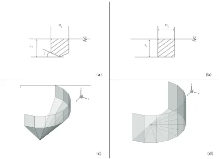
Following the past introduced theory, the next section will introduce different case scenarios (Figure

2):

a

L L

D D

a

c

c

ζ

(a) (b)

(c) (d)

Figure 2.Section Views (a),(b) and Isometric Views (c),(d) on the two Point Absorber types

Last figure depicts on its upper part (Subfigures a-b) the sectional sketches of the given cases. One can notice that only the wet part of the bodies is shown, for the reason that it is the only relevant part in the BEM calculation. On the lower part (Subfigures c-d) merely one half of the given bodies is exposed. This is due to the fact, that all bodies are axisymmetric, and for the initial configuration only one half around the xz - symmetry plane needs to be modeled in order to obtain the hydrodynamic coefficients. It is noted that in all three cases, the incoming wave direction is the positive x-axis. For a single body, the cone cylinder case in (a) and (c) initially serves to validate the chosen model approaches of radiation and excitation in heave. Finally, the generic vertical floating cylinder case study in (b) and (d) will lead to conclusions on the interaction of several units with variable distancelλ between them in different

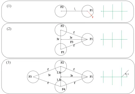
array layout configurations [32], such as the ones depicted in the following Figure3:

(1)

(2)

(3)

F1 F1

F1 F2

F2

F2 F3

F3

l_λ

3r 3r

1.5r

3r 3r

r

f

f

f

f f

f 1.5r

F3

F4

ß

Figure 3.Top View sketch for the three investigated PA array layouts

keeping the bodies more stretched in the x-direction than in the y one. The reason for choosing latter cases relies on the results determined by [39,40], which refer to that triangular and squared/diamond array layouts as fairly suited for Ocean Wave Energy extraction [41].

2.4. Simulation parameters

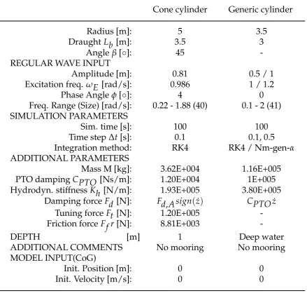
The next endorsed Table2summarizes effectively the parameter configuration for the simulation runs.

According to the table both cases are calculated in Scale 1:1. Only the first one is then sized down for Post-Processing through Froude scaling laws to 1:15.9, which is the scale of the experimental setup in de Backer’s (GdBck) thesis [18]. This becomes part of the first analyzed task as described in the next section. From this step on, the researcher will use the results delivered by the BEM code NEMOH according to the geometries chosen next. It is noted though, that for multiple bodies, a sensitivity analysis of the time step takes place, and values are placed linearly in between 0.1sand 0.5son a 0.05sstep base, resulting in 0.5sas best case scenario. Reference here for has been previous work done in thesis delivered by [18,29].

3. Results

Table 2.Simulation parameters

Cone cylinder

Generic cylinder

Radius [m]:

5

3.5

Draught

_Lb

[m]:

3.5

3

Angle

β

[

◦

]:

45

-REGULAR WAVE INPUT

Amplitude [m]:

0.81

0.5 / 1

Excitation freq.

ω

_E

[rad/s]:

0.986

1 / 1.2

Phase Angle

φ

[

◦

]:

4

0

Freq. Range (Size) [rad/s]:

0.22 - 1.88 (40)

0.1 - 2 (41)

SIMULATION PARAMETERS

Sim. time [s]:

100

100

Time step

∆

t

[s]:

0.1

0.1, 0.5

Integration method:

RK4

RK4 / Nm-gen-

α

ADDITIONAL PARAMETERS

Mass M [kg]:

3.62E+004

1.16E+005

PTO damping

_CPTO

[Ns/m]:

1.20E+004

1E+005

Hydrodyn. stiffness

_Kh

[N/m]:

1.93E+005

3.80E+005

Damping force

_Fd

[N]:

_Fd

_,

_{A sign}

(

z

˙

)

_CPTO

z

˙

Tuning force

_Ft

[N]:

1.20E+005

-Friction force

_{Ff r}

[N]:

8.81E+003

-DEPTH

[m]

1

Deep water

ADDITIONAL COMMENTS

No mooring

No mooring

MODEL INPUT(CoG)

Init. Position [m]:

0

0

Init. Velocity [m/s]:

0

0

The following analysis is being subdivided into a function of the number of bodies under study. First, the single cases of the cone cylinder and the generic floating cylinder are discussed. Then, the behavior of arrays of up to four generic PA(s) are documented.

3.1. One floating body

3.1.1. Cone cylinder in heave

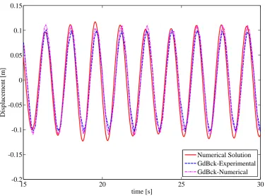
The cone cylinder study is related to latter introduced FO3-Buldra project. Its calculation leads to the following Figure4.

15 20 25 30 -0.2

-0.15 -0.1 -0.05 0 0.05 0.1 0.15

time [s]

Displacement [m]

Numerical Solution GdBck-Experimental GdBck-Numerical

Figure 4.Cone cylinder case - Results Validation

certain amplitude modulation over the interval. All over the peaks and troughs, the numerical results deliver higher amplitudes than the experimental results. In general, there is≈ 16.67% max. deviation from the experiments displacement. However, the phase is nearly matched by the numerical results, which in the original thesis delivered as well higher amplitudes than the test setup. Hence, one can compare the numerical solution with the one obtained by de Backer (cf. dashed magenta curve) [18]. It can be noticed, that its numerical solution also peaks over the experimental results, exhibiting a sort of amplitude modulation, which behaves in a very similar fashion to the presently obtained solution.

3.1.2. Generic cylinder in heave

In addition to the previous, the following generic cylinder case serves as a base for an immersion into the parametric of geometrical and hydrodynamic variables, as it will be seen next.

3.1.3. Capture width in heave mode

10 10.5 11 11.5 12 12.5 13 101

Wave Period [s]

CW [m]

CW Babarit [m] CW Price [m]

10 10.5 11 11.5 12 12.5 13 100

Wave Period [s]

CWR [-]

CWR Babarit [-] CWR Price [-]

Figure 5. Comparative of applied methods on capture width determination for the default generic floating vertical cylinder

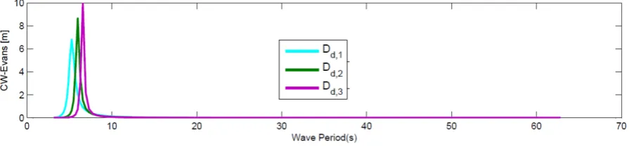
In Figure 5 one can distinguish either capture width values denoted with Cw [in m] or capture width ratiosCWR[dimensionless] for the default draught ofDd,1=3m. With relationship to the wave frequency, theCw never exceeds a ratio greater than 0.5, while there is a significant agreement in the methods presented by Babarit and Price, specially for the highlighted wave period range of 11-13 s.

Figure 6.Capture width as a function of variable draught

3.1.4. Multiple degrees of freedom

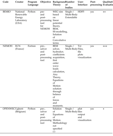
The incorporation of the BEMIO package for a single floating body case leads to a full calculation of its hydrodynamic coefficients, together with some transformations in the state-space modeling part through the use of the NEMOH tool. While the first package is a Python oriented program for the array calculation in multiple degrees of freedom, the second application contains a FORtran based code for the hydrodynamic parameter acquisition, among other capabilities. Further details are outlined in the following table3:

Table3reflects a qualitative assessment ranging from one plus to three plus units depending on its performance capabilities. The criteria behind is simply the flexibility in order to be able to adapt the code to specific problems, as well as its performance in terms of quality and time consumption. OpenWEC, e.g. is the newest code, and reveals itself pretty handy in terms of user interface parametrization, but presents lacks of adaptability to modify the available package. On the opposite, NEMOH has proven to be able to cope with WAMIT performance [54], while providing multiple ways to redefine procedures and therefore obtains the highest evaluation mark.

Table 3.Hydrodynamic packages assessment

Code Creator Program Language Objective Background Theory Number of bodies User-Interface Post-processing Qualitative Evaluation BEMIO National Renewable Energy Laboratory (USA) Python pre-and post-processing tool for NEMOH WEC-sim based on linear potential theory, BEM, SS-modelling, Solution of Convolutive terms Single-/ Multi-Body Extendable

HDF5 yes ++

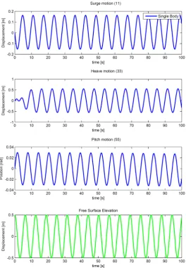
Figure 7.Resulting PA motion for the regular waves case

As it can be seen on Figure7, the results remain consistent for the heave mode, since nothing with regard to the integration method (time step or sim. time) has been modified. Additionally, one obtains a surge component of max. 0.17m, min.−0.17m, which explains why the buoy shifts horizontally during excitation and resulting oscillation. Also, there follows a consequent pitching moment along the rotation axis of the buoy, revealing values up to max. 0.03 rad and down to min. -0.03 rad.

3.2. Multiple floating bodies in heave

For this part of the paper, the generic floating cylinder remains under consideration. Used for instance in CFD simulations [45–47], this type of geometry has become as well predominant in the published literature on BEM calculations [48,49]. From this stage on, the study presents only the results related to interacting cylinders in the configurations highlighted in Figure3.

3.2.1. Two generic cylinders (aligned)

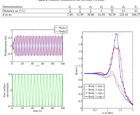
At this stage, two separated, aligned bodies with the wave direction are exposed initially to regular waves of 0.5 m amplitude. The distancedis varied according to the wavelengthλ, which is calculated

for deep water waves through the relationshipωE =1 Hz⇒T=6.28 s, henceλ ∼=1.56T2=61.59 m.

Table 4.Distance variations in the two body PA study

Denomination d1 d2 d3 d4 d5 d6 d7

Distance asf(λ) λ₈ λ₄ λ₂ λ 3₂λ 2λ 3λ

d in m 7.69 11.59 30.80 61.59 92.39 123.18 184.77

0 20 40 60 80 100

-1 -0.5 0 0.5 1

time [s]

Displacement [m]

Body1 Body2

0 20 40 60 80 100

-0.5 0 0.5

time [s]

Free surface _elevation[m]

(a)(Top) Displacement reaction of bodies 1-2, (Bottom) Surface Elevation [ωe,1,C1]

0 0.5 1 1.5 2

0 0.2 0.4 0.6 0.8 1 1.2 1.4 1.6 1.8 2

 in [Hz]

RAO [-]

Body 1 (init.) Body 2 (init.) Body 1 (opt.) Body 2 (opt.)

(b)RAO’s forC1andCOptfor a variable frequency range

For d1-d7one obtains from Eq. (14) the same eigenfrequency ofω0 = 1.2Hzfor each one of the bodies in every distance case. Again,z, ˙z, ¨z, RAO’s andPaare computed for both bodies. For sake of conciseness, merely one distance calculation is outlined. It refers to distanced3, which is half the wave length between the two cylinders. The results are observed in the following set of Figures8aand8b:

conditions on the other hand, it is body 2 which shadows body 1 predominantly over the frequency range of 1.25−1.5Hz.

Another way of interpreting the oscillation amplitude ˆz can be extracted from the following diagrams (Figs.8,10).

Figure 9.Amplitude ratio zˆj ˆ

z0for each j-body in relation to single body forωe,1,Aw,1andC1

Finding reference in Earthquake Engineering [50], a method has been determined for variable distances, which delivers amplitude amplification ratios for each body with respect to the isolated body case. These ratios are not be confused with RAO’s though their curve shapes are particularly similar. Limitation to these novel ratios are given generally for irregular waves, since the amplitude in the displacement varies continuously due to the superposition of waves. The graphs reflect for a fixed frequency and variable distances on the horizontal axis the ratio of the maximum amplitude for each body ˆzj to the amplitude of the isolated body case ˆz0 on the vertical axis. For Figure8a this means, that having ˆz0=0.64m, the amplitude amplification ratio becomes zˆ1

ˆ

z0 =0.938 (body 1) and ˆ z2 ˆ

z0 =0.984 (body 2), which are the points on the vertical dashed line for_λd =0.5. On Figure8one can also observe, that there is amplification in the movement of the devices, if both bodies oscillate above the horizontal dashed limit of _zz_ˆˆj

0 = 1. For instance, the distancesd2andd4show amplification ratios above one for both bodies. For the first mentioned distance value of_λd =0.25, zˆ1

ˆ

z0 =2.35 and ˆ z2 ˆ

z0 =1.05, meaning that although the first body receives clearly more energy, the second still gets some motion amplification. This also happens to be the case for _λd = 1, where zˆ1

ˆ z0 =

ˆ z2 ˆ

Figure 10.Amplitude ratio zj

z0for each j-body in relation to single body forωe,1,Aw,1andCOpt

Latter graph reflects only ten operative points from the twelve studied distance cases. This is due to diverging simulations for the initial time step of 0.1 s. However, one can deduce a similar behavior to latter curves, having amplified displacements close to d_λ = 0.15, (with zˆ1

ˆ

z0 =1.4 and ˆ z2 ˆ

z0 =1.1) and close tod_λ =0.2, (withzˆ1

ˆ

z0 =1.35 and ˆ z2 ˆ

z0 =1). Again, the curve tends to decay for increasing distances. Further studies need to be done for an optimum excitation frequency in near resonance conditions with the same optimum damping in order to validate this part of the study. Its result is shown in Figure10, with ten operative working points, where a significant amplification ratio at d_λ =0.75 can be appreciated. Here,

ˆ z₁

ˆ z0 ≈

ˆ z2

ˆ

z0 ≈2.5, achieving maximum amplification of nearly five times the incident wave amplitudeAw,1.

Figure 11.Amplitude ratio zˆj ˆ

z0for each j-body in relation to single body forωe,2,Aw,1andCOpt

For the interaction of cases 2 and 3 in Figure3, the two integration methods of RK4 and Nm− gen−αare compared against each other for the displacement in 1 m high waves.

3.2.2.Three generic cylinders (triangular disposition)

0 10 20 30 40 50 60 70 80 90 100 -2

0 2

time [s]

Displacement [m]

Body1-RK Body1-Newmark

0 10 20 30 40 50 60 70 80 90 100

-0.5 0 0.5

time [s]

Displacement [m]

Body2-RK Body2-Newmark

0 10 20 30 40 50 60 70 80 90 100

-0.5 0 0.5

time [s]

Displacement [m]

Body3-RK Body3-Newmark

Figure 12. Displacement for the triangle configuration of bodies 1-3 over two different integration methods

It can retraced from11, there is a matching of results for the two integration methods applied with regard to body 1. Bodies 2 and 3 experience a minimum delay of second decimals in the Newmark approach, which can be related to the difference in time step employed, or simply due to the matrix inversion calculation. However, amplitudes seem to be approximated properly, so that the methods are also being applied on four separated bodies next.

3.2.3.Four generic cylinders

Two main separate subcases are analyzed in the following subsections, namely the squared and diamond disposition according to the layout from case3. For each subcase, the heave displacement (acc. to previous applied integrational methods), is presented selectively [case 3].

Squared disposition

Being characterized by the fact, that the perpendicular distance between each body is equal to f (acc. to the rombus diagonal), the layout is taken from the Case studies, such that Floaters 1-4 appear counter-clockwise, starting from the east-left position. This way, 9 different incident angles are tested (β = 0, 25,45, 60,90, 120, 135, 155,180), and the bold highlighted cases are detailed in the following.

Reason therefore is, that there is some expectation in advance, of at least what should be the amplitude tendency within the bodies response [B,1] to [B,4]

Subcase 1: beta=0 [Figures12and13]

Motion amplitude assessment:(zˆB,2∼=zˆB,4)<<(zˆB,3>zˆB,1) Subcase 2: beta=45 [Figures14and15]

0 10 20 30 40 50 60 70 80 90 100 -2

-1.5 -1 -0.5 0 0.5 1 1.5 2

time [s]

Displacement [m]

Body 1 Body 2 Body 3 Body 4

0 10 20 30 40 50 60 70 80 90 100

-0.5 0 0.5

time [s]

Free surface elevation[m]

Figure 13.(Left) displacement for all floaters 1-4 in square[beta=0]

0 10 20 30 40 50 60 70 80 90 100

-2 -1 0 1 2

time [s]

Displacement [m]

Body1-RK Body1-Newmark

0 10 20 30 40 50 60 70 80 90 100

-1 -0.5 0 0.5 1

time [s]

Displacement [m]

Body2-RK Body2-Newmark

0 10 20 30 40 50 60 70 80 90 100

-2 -1 0 1 2

time [s]

Displacement [m]

Body3-RK Body3-Newmark

0 10 20 30 40 50 60 70 80 90 100

-2 -1 0 1 2

time [s]

Displacement [m]

Body4-RK Body4-Newmark

Figure 14.Separate displacements for the integrational variation methods[beta=0]

Subcase 3: beta=90 [Figures16and17]

Motion amplitude assessment:(zˆB,1∼=zˆB,3)>(zˆB,2>zˆB,4) Subcase 4: beta=180 [Figures18and19]

0 10 20 30 40 50 60 70 80 90 100 -0.8

-0.6 -0.4 -0.2 0 0.2 0.4 0.6 0.8

time [s]

Displacement [m]

Body 1 Body 2 Body 3 Body 4

0 10 20 30 40 50 60 70 80 90 100

-0.5 0 0.5

time [s]

Free surface elevation[m]

Figure 15.(Left) displacement for all floaters 1-4 in square[beta=45]

0 10 20 30 40 50 60 70 80 90 100

-1 -0.5 0 0.5 1

time [s]

Displacement [m]

Body1-RK Body1-Newmark

0 10 20 30 40 50 60 70 80 90 100

-1 -0.5 0 0.5 1

time [s]

Displacement [m]

Body2-RK Body2-Newmark

0 10 20 30 40 50 60 70 80 90 100

-1 -0.5 0 0.5 1

time [s]

Displacement [m]

Body3-RK Body3-Newmark

0 10 20 30 40 50 60 70 80 90 100

-1 -0.5 0 0.5 1

time [s]

Displacement [m]

Body4-RK Body4-Newmark

Figure 16.Separate displacements for the integrational variation methods[beta=45]

0 10 20 30 40 50 60 70 80 90 100 -1

-0.5 0 0.5 1

time [s]

Displacement [m]

Body 1 Body 2 Body 3 Body 4

0 10 20 30 40 50 60 70 80 90 100

-0.5 0 0.5

time [s]

Free surface elevation[m]

Figure 17.(Left) displacement for all floaters 1-4 in square[beta=90]

0 10 20 30 40 50 60 70 80 90 100

-2 -1 0 1 2

time [s]

Displacement [m]

Body1-RK Body1-Newmark

0 10 20 30 40 50 60 70 80 90 100

-1 -0.5 0 0.5 1

time [s]

Displacement [m]

Body2-RK Body2-Newmark

0 10 20 30 40 50 60 70 80 90 100

-2 -1 0 1 2

time [s]

Displacement [m]

Body3-RK Body3-Newmark

0 10 20 30 40 50 60 70 80 90 100

-1 -0.5 0 0.5 1

time [s]

Displacement [m]

Body4-RK Body4-Newmark

Figure 18.Separate displacements for the integrational variation methods[beta=90]

Diamond disposition

0 10 20 30 40 50 60 70 80 90 100 -2

-1.5 -1 -0.5 0 0.5 1 1.5 2

time [s]

Displacement [m]

Body 1 Body 2 Body 3 Body 4

0 10 20 30 40 50 60 70 80 90 100

-0.5 0 0.5

time [s]

Free surface elevation[m]

Figure 19.(Left) displacement for all floaters 1-4 in square[beta=180]

0 10 20 30 40 50 60 70 80 90 100

-1 -0.5 0 0.5 1

time [s]

Displacement [m]

Body1-RK Body1-Newmark

0 10 20 30 40 50 60 70 80 90 100

-2 -1 0 1 2

time [s]

Displacement [m]

Body2-RK Body2-Newmark

0 10 20 30 40 50 60 70 80 90 100

-2 -1 0 1 2

time [s]

Displacement [m]

Body3-RK Body3-Newmark

0 10 20 30 40 50 60 70 80 90 100

-2 -1 0 1 2

time [s]

Displacement [m]

Body4-RK Body4-Newmark

Figure 20.Separate displacements for the integrational variation methods[beta=180]

4. Discussion

Next, it is the capture width for the generic vertical cylinder PA, which ensures, that the case is analog to what can be found in the literature. The research concludes, this study can be easily parametrized into configurations of two, three or four interacting floaters with various frequencies and/or distances. It is being noted again, that the Post-Processing of results has been reduced to specific distance and frequency cases, in order not to exceed the scope of this publication. Despite of this, several aspects can be highlighted from the commented simulation runs. For the three introduced problems of varying frequency and PTO damping (ωe,1,ω0andCOpt), the computation diverges at specific distances for the chosen initial time step of 0.1 s. However, a variation of the time step, choosing for instance 0.5 s achieves convergence. This generates a conflict in the sense, that the explicit scheme used initially, presents only preliminary accuracy for 1-2 buoys. However, for three or more floating bodies, the implicit scheme shows at least more suitable results for 0.5 s time step, while the explicit scheme with any time step < 0.5 s does not converge at all. The before mentioned conflict relies on the experience, that generally speaking, explicit integration methods require smaller time steps than implicit ones, leading to less stability. In the distance range d_λ = 0−0.5 interactions seem to be more intense for all three cases. These might be due to near-trapping effects. Afterward, the curves tend to decay with distance. This behavior has been documented in the literature [34]. There is an existing proportionality between the increase of wave amplitude and the displacement of the bodies, which is explained through linear potential theory. With optimum damping, the amplitude in the displacement for a single body increases significantly. This increase is maximal, whenωe =ω0. For this case, the displacement nearly quadruplicates the wave amplitude, as the RAO shows. As expected for intermediate distances, the bodies move in counter-phase (0.5λ, 1.5λ... (n-0.5)λ), while they are in phase for odd values ofλ(λ, 3λ

... (2n-1)λ)

Summing up, the perspective for future research is enlightening. For a single cylinder, optimum fitting should be regarded primarily with respect to draft adjustment and PTO damping. Not only could there be application of CFD studies, but also experimental testing to any of the given cases. Moreover, capture width ratios should be determined, in order to be able to calculate the system(s) efficiency. For the problems of 3-4 cylinders, one can foresee how greater array configurations may be designed according to the presented principle. Finally, it is the q-factor study which could be optimized for Arrays, by carrying out simulations for various distances and a fixed optimum frequency. Main issue during this study remains the subject of presenting specific results for irregular waves due to the lack of field data for this PA types, where it becomes really difficult to understand phenomena such as shadowing effects, etc. Besides, the displacement discrepancy of floaters 2-4 in Figures 13 - 17 requests deeper knowledge on the applied numerical packages, and are therefore out of this research scope.

5. Conclusions

During the course of this research, a number of milestones have been achieved. First of all, for both unidirectional regular or irregular waves, a solid, flexible, transparent and computationally efficient W2M model has been provided.

With respect to the Single Cylinder analysis it can be said that both time and frequency domain solutions have been verified and correlate for different wave amplitudes, excitation frequencies and PTO Damping values. Although the case has been elucidated for both regular and irregular waves as an input, for the multiple bodies scenario the restriction to simple regular waves as an input has been kept in order to better understand how interactions work. Additionally, it is the use of packages such as BEMIO or OPENWEC, which open new perspectives for the investigation of multiple degrees of freedom.

1. Correlation between the increase of wave amplitude and the displacement of the bodies, which is explained through linear potential theory

2. Optimum PTO Damping nearly doubles the displacement of the two bodies, increasing interaction. This is verified in the literature [23,35,51].

3. As it is expected, for intermediate wave lengths the bodies move in counter-phase (0.5λ, 1.5λ..

(n-0.5)λ), while they are in phase for odd values ofλ(λ, 3λ.. nλ)

The triangle configuration itself turns out to be the a suitable choice in terms of Wave Energy extraction for small arrays according to literature [41,51]. Out of this recent references it is also worth to investigate results for greater arrays. In the present research, it can be appreciated, that F1 facing the incoming wave receives an amplitude amplification in displacement which nearly doubles the wave amplitude. Besides, the two remaining cylinders in the background keep moving synchronously, with a displacement minimally lower than the incident wave. The only possible reason points towards floaters 2-3 feeding back at F1 through radiation processes, which need to be studied more carefully. Albeit, the two applied integration methods (RK4 andNm−gen−α) are relatively in concordance, validating

this way the research study. Despite this fact, it is recommendable to rather take advantage of implicit schemes only while modeling multiple bodies for the reasons exposed during the discussion section. Elsewhere, the application of explicit schemes might reveal itself more appropriate in terms of accuracy. Last but not least, it is the park effect which is pointed out for showing the interactions in the 4-cylinders

• Square

There is, despite some discrepancy in the amplitude results, quite an agreement within the symmetrical boundaries for this configuration. For beta 0 and 180, there is an opposed behavior within the floater numbers, which is expected though. Also for beta=45, the side floaters to the wave front get more input than the ones fronting the wave. The 90 degrees incidence case merely validates the previous cases, since it is again floaters 1 and 3 located laterally to the wave train, the ones that are significantly amplified.

• Diamond

Although the results present a different shape to what has been done up to now in the field, there appears to be constructive interference for a wide range of combined frequencies and incident angles. Moreover, symmetry around the perpendicular from the top coming incident angle of 90◦ confirms the expected behavior of the four floaters. It presents nearly the same interaction for the cases, where the wave train originates either from the right (0 degrees) or the left (180 degrees) of the diamond configuration. Furthermore, there is a decaying tendency for an increasing frequency, both facts that have been dealt with before in the given references.

The complexity of the studied case leaves a broad margin for future investigation and optimization strategies. Hydrodynamic aspects, which are worth to set focus on in the near future, are e.g. geometry modification strategies, application of mooring configurations, behavioral study of shadowing / near-trapping effects, consequences of extreme waves events and last but not least, the improvement of capture width ratios by means of the first three preceding characteristics. With regard to this, it is noted, that recent research reveals and confirms the right choice of the generic PA geometry during the present investigation [53]. Hence, it is consistent to assert, that it is the combination of the cylindrical shape with a functional bottom shape, which will surely provide future insights about the performance optimization within the point absorber technology field.

1involving e.g. Fractal and quantum theory [55] . They are of primary importance, since studying fluids up to date has revealed itself a task of looking deep into the details, as CFD or Smooth Particle Hydordynamic simulations show. Besides, the application of existing formulations, such as the Helmholtz’s wave equation, combined with the existing boundary conditions and Airy theory might enhance new paths for investigation. Focusing furthermore on the energy perspective, it may be even partially possible to bypass or compensate the balance of forces. While neglecting the related sort of uncertainties given in its relationships and assuming the whole as a computational approach, neural networks might set up an innovation breakline both for the estimation of statistics and probability of the PA’s overall performance. In other words, it might be determining to consider the system wave to motion in computer science terms aBig Dataunit [56] with regard to real sea conditions. Latter one might enable to draw knowledge from a waves database history, resulting in being able to link different affected mathematical and physical scenarios, such as irregular waves handling, wave state prediction or extreme events execution.

Acknowledgments: The author would hereby like to thank the economical support granted since January 2016 through the company CIB labs. Also, fundamental contributions to the theoretical and practical implementations within this study by Aurelien Babarit, Griet de Backer, Bret Bosma, Peter Frigaard and Luis A. Padron are truly appreciated. More generally, all help provided through the NEMOH user forum is respected as well. Finally, the aid for addons and corrections provided through Emperador Alzola’s supervision is truly estimated.

Conflicts of Interest:The author declares no conflict of interest. Abbreviations

The following abbreviations are used in this manuscript:

BEM Boundary Element Method

CFD Computational Fluid Dynamics FRACT Fractal Theory

LHS, RHS Left, right hand side

MSD Mass-Spring-Damper

PA Point Absorber

PTO Power Take-Off

QUANT Quantum Mechanics

RAO Response Amplitude Operator

STRUC Structural Vibrations

WEC Wave Energy Converter

W2M Wave-to-motion

W2W Wave-to-wire

Symbol Description Dimension

A Added mass [kg]

Ai,j Added mass matrix [kg]

Ar Added mass for

Radiation

[kg]

Ar,∞ Added mass at infinite frequency

[kg]

Aw Wave amplitude [m]

β Incident Wave

direction

[degrees]

βG,γG Numerical stabilizing parameters for Newmark generalized alpha integration method

Ch Radiation Damping [kgs ]

cw Capture width [m]

cpto PTO-damping [kg_s ]

d Draft [m]

db Diameter of the buoy [m]

Dh Water depth (h) [m]

η Free surface elevation [m]

Ed Spectral energy

density

[_mW₂]

Ef Energy flux [kWm]

Fh Hydrostatic restoring

force

[N]

Fpto PTO-force [N]

Fe Excitation force [N]

Fd Diffraction force [N]

Ff k Froude-Krylov force [N]

Fw Wave force [N]

Fm Mooring force [N]

Fr Radiation force [N]

g Gravitation constant [m_s2]

H Wave height [m]

Hs Significant wave

height

[m]

i,j Matrix indexes for the six degrees of freedom

λ wave length

l Point absorber length [m]

k Wave number []

kr Retardation kernel [N]

Kh Hydrostatic stiffness [kg_s2]

L Wave length [m]

Mf Floater mass [m]

Mt Total mass [m]

~n Normal vector [−]

nk cosine direction of

surface elevation

[degrees]

ω Circular wave

frequency

[Hz]

ωp peak frequency [Hz]

Pa Absorbed power [W]

Pe Exciting power [W]

Pr Radiation power [W]

Parr Array power [W]

Piso Isolated single body power

[W]

q Interaction factor [−]

ρ Water density [_mkg3]

σ angular frequency [Hz]

τ Time span [s]

ν radiation potential [−]

uxi potential flow velocity [ m

s]

U complex velocity

magnitude

[−]

v flow velocity [m_s]

ξ cone slope [degrees]

z, ˙z, ¨z Displacement,

velocity and acceleration in heave

[m,m_s,m_s2]

Z Displacement

magnitude

[−]

References

1. Magagna, D.; Uihlein, A. Ocean Energy Status Report: Technology, market and economic aspects of ocean energy in Europe. 2014 JRC, 2015. Report EUR 26983 EN.

2. Budal, K.; Falnes, J. A resonant point absorber of ocean-wave power. Nature 256: pp. 478-479, 1975. doi:10.1038/256478a0.

3. Evans, D.V. A theory for wave-power absorption by oscillating bodies. Journal of Fluid Mechanics 77 (1): 1–25, 1976. doi:10.1017/S0022112076001109.

4. Villate, J.L.; Brito e Melo, A. Annual Report Ocean Energy Systems 2016. The Executive Committee of Ocean Energy Systems, 2016. https://report2016.ocean-energy-systems.org

5. Marquis, L.; Kramer, M.; Frigaard, P. First Power Production figures from the Wave Star Roshage Wave Energy Converter. 3rd International Conference on Ocean Energy ICOE, 2010.

6. Iuppa C., Cavallaro L., Vicinanza D., and Foti E. Investigation of suitable sites for Wave Energy Converters around Sicily (Italy) Ocean Sci., 11, 543-557, 2015, doi: 10.5194/os-11-543-2015.

7. De Rouck, J. SEEWEC, A promising WEC : multiple point absorbers in a floating platform. EC contractors meeting, Bremerhaven, 2006.

8. Merino, J.; Veganzones, C. Power system stability of a small sized isolated network supplied by a combined wind-pumped storage generation system: A case study in the canary islands. Energies Volume 5, Issue 7, Pages 2351-2369, 2012.

9. Stoutenburg, E.; Jenkins, N.; Jacobson, M. Power Output Variations of Offshore Wind Turbines and Wave Energy Converters in California. Renewable Energy, 2010.

10. Banos Hernandez, L.; Emperador Alzola, L. Hydrodynamic Assessment on Motion Performance characteristics of generic wave energy point absorbers. IJETMR: International Journal of Engineering Technology and Management Research, 2017. Volume 4, Issue 23.

11. Li, Y.; Yu, Y.H. A synthesis of numerical methods for modeling wave energy converter-point absorbers. Renewable and Sustainable Energy Reviews 16, pages 4352– 4364, 2012.

12. Koomey, J.; Berard, S.; Sanchez, M.; Wong, H. IEEE Annals of the History of Computing, 33, 3, 46–54., 2011. Article number 5440129.

13. Garcia-Rosa, P.; Cunha, J.; Lizarralde, F.; Estefen, S.; Machado, I.R.; Watanabe, H. Wave-to-wire model and energy storage analysis of an ocean wave energy hyperbaric converter. IEEE Journal of Oceanic Engineering, 2014.

14. Falnes, J. Ocean Waves and Oscillating Systems: Linear Interactions Including Wave - Energy Extraction. Cambridge University press, 2002. ISBN 982-207-002-0.

17. Banos Hernandez, L.; Frigaard, P.; Kirkegaaard, P. Numerical modeling of a wave energy point absorber. Proceedings of the Twenty Second Nordic Seminar on Computational Mechanics, 2009. Aalborg University | ISSN 1901-7278 DCE Technical Memorandum No. 11.

18. de Backer, G. Hydrodynamic Design Optimization of Wave Energy Converters Consisting of Heaving Point Absorbers. Ghent University, 2012. PhD thesis, pp. 103-104.

19. Eriksson, M.; Waters, R.; Svensson, O.; Isberg, J.; Leijon, M. Wave power absorption: Experiments in open sea and simulation. Journal of Applied Physics 102, 084910, 2007.

20. Bosma, B. On the Design, Modeling, and Testing of Ocean Wave Energy Converters. Oregon State University, 2013. PhD thesis, pp. 40-41.

21. Evans, D.; Porter, R. Near-trapping of waves by circular arrays of vertical cylinders. Applied Ocean Research 19, pp. 83-99, 1997.

22. McIver, P. Wave interaction with arrays of structures. Applied Ocean Research 24 121–126, 2002.

23. Garnaud, X.; Mei, C. Comparison of Wave Power Extraction by a Compact Array of Small Buoys and by a Large Buoy. IET Renewable Power Generation, Volume 4, Issue 6, pages 519-530, 2010.

24. Perez, T.; Fossen, T. Seakeeping Models in the Frequency Domain. One-day Tutorial, CAMS 07, Bol, Croatia, 2007.

25. Fossen, T. Guidance and control of ocean vehicles. John Wiley and Sons Ltd, 1994. ISBN 0-471-94113-1. 26. Faltinsen, O.M. Sea Loads on Ships and Offshore Structures. Cambridge University Press, 1990. ISBN 0 521

45870.

27. Taghipour, R.; Perez, T.; T., M. Hybrid frequency–time domain models for dynamic response analysis of marine structures. Ocean Engineering 35, pages 685–705, 2008.

28. Yu, Z.; Falnes, J. State-Space modelling of a vertical cylinder in heave. Applied Ocean Research 17, pages 265-215, 1995.

29. Alves, M. Numerical Simulation of the dynamics of Point Absorber Wave Energy Converters using frequency and time domain approaches. Universidade Tecnica de Lisboa, 2012. PhD thesis.

30. Clement, A.; Babarit, A. Discrete control of resonant wave energy devices. Philosophical Transactions of the Royal Society A: Mathematical, Physical and Engineering Sciences Vol. 370, Issue 1959, pages 288-314, 2012. 31. R., R.; J., S.; T., P. Time-domain models and wave energy converters performance assessment. 27th

International Conference on Offshore Mechanics and Arctic Engineering, pp. 1-10, 2008.

32. Babarit, A. A database of capture width ratio of wave energy converters. Renewable Energy 80, pp. 610-628, 2015.

33. Falcao, A. Wave energy utilization: A review of the technologies. Renewable and Sustainable Energy Reviews 14, 2010.

34. Child, B. On the configuration of arrays of floating wave energy converters. The University of Edinburgh, 2011. PhD thesis.

35. Babarit, A. On the park effect in arrays of oscillating wave energy converters. Renewable Energy 58, 2013. 36. Cruz, J. Ocean Wave Energy - Current Status and Future Perspectives. Springer Verlag, 2008.

978-3-540-74894-6.

37. Wolgamot, H.; Eatock Taylor, R.; Taylor, P.H. The interaction factor and directionality in wave energy arrays. Ocean Engineering Volume 47, 2012.

38. Bellew, S.; Stallard, T.; Stansby, P. Optimisation of a Heterogeneous Array of Heaving Bodies. University of Manchester, UK, 2013.

39. Borgarino, B.; Babarit, A.; Ferrant, P. Impact of wave interactions effects on energy absorption in large arrays of wave energy converters. Ocean Engineering 41, pp. 79–88, 2012.

40. De Andres, A.; Guanche, R.; Meneses, L.; Vidal, C.; Losada, I. Factors that influence array layout on wave energy farms. Ocean Engineering Volume 82, Pages 32-41, 2014.

41. Moarefdoost, M.M.e.a. Layouts for ocean wave energy farms: Models, properties and optimization. Omega 66, pp.185–194, 2016.

43. Price, A.; Dent, C.; Wallace, A. On the capture width of wave energy converters. Applied Ocean Research, 2009. Vol. 31, pp. 251-259.

44. Lewis, A.; Alcorn, R.; Sheng, W. On improving wave energy conversion, part I: Optimal and control technologies. Renewable Energy, 2015. Vol. 75, pp. 922-934.

45. Agamloh, E.; Wallace, A.; von Jouanne, A. Application of fluid–structure interaction simulation of an ocean wave energy extraction device. Renewable Energy 33, pp. 748–757, 2008.

46. Yi-Hsiang Yu, Y.L. Reynolds-Averaged Navier–Stokes simulation of the heave performance of a two-body floating-point absorber wave energy system. Computers and Fluids 73, pp. 104–114, 2013.

47. Paredes, G.; Eskilsson, C.; Palm, J.; Bergdahl, L.; Leite, L.; Taveira-Pinto, F. Experimental and Numerical Modelling of a Moored, Generic Floating Wave Energy Converter. 10th European Wave and Tidal Energy Conference, 2013.

48. Eriksson, M.; Isberg, J.; Leijon, M. Hydrodynamic modelling of a direct drive wave energy converter. International Journal of Engineering Science 43, pp. 1377–1387, 2005.

49. Falnes, J.; Hals, J. Heaving buoys, point absorbers and arrays. Phil. Trans. R. Soc. A, Vol. 370, 246–277, 2012. 50. Hong-Wen Maa, H.W.; Shao-Ming, Y.; Li-Quan, W.; Zhong, Z. Analysis of the displacement amplification ratio

of bridge-type flexure hinge. Elsevier Sensors and Actuators A: Physical, 2006. Volume 132, Issue 2, Pages 730–736.

51. Liu, H.e.a. Wave Energy conversion by cylinder array with a floating platform considering linear/nonlinear PTO damping. J Mar Sci Technol, 2017.

52. Newmark,N.M. A Method of Computation for Structural Dynamics ASCE Journal of Engineering Mechanics Division, Vol 85. No EM3, 1959. http://opensees.berkeley.edu/wiki

53. et al., Z.W.C. Hydrodynamic Analysis and Shape Optimization for Vertical Axisymmetrix Wave Energy Converters. China Ocean Eng., Vol. 30, No. 6, pp. 954 – 966, 2016.

54. Penalba, M. et al. Using NEMOH for Modelling Wave Energy Converters: A Comparative Study with WAMIT. Centre for Ocean Energy Research (COER), Maynooth University, Co.Kildare, Ireland, 2017.

55. Cabrera, L. Analisis fractal de procesos dinamicos en el oceano Phd Thesis, ULPGC, 2003