Article
1
Coatings Thickness Determination Using X-ray
2
Fluorescence Spectroscopy: Monte Carlo Simulations
3
as an Alternative to the Use of Standards
4
Walter Giurlani 1,*, E. Berretti 2, Massimo Innocenti 1.2 and Alessandro Lavacchi 2,*
5
1 Dipartimento di Chimica, Università degli Studi di Firenze, via della Lastruccia 3, 50019 Sesto Fiorentino
6
(FI), Italy; [email protected]
7
2 Consiglio Nazionale delle Ricerche—Istituto di Chimica dei Composti OrganoMetallici (CNR-ICCOM),
8
via Madonna del Piano 10, 50019 Sesto Fiorentino (FI), Italy
9
* Correspondence: [email protected] (W.G.); [email protected] (A.L.);
10
Tel.: +39-055-457-3102 (W.G.); +39-055-522-5250 (A.L.)
11
12
Abstract: X-ray fluorescence is largely employed in the measurement of the thickness of coatings.
13
Despite of its diffusion, the task is not straightforward because of the complex physics involved that
14
results in high dependence on matrix effects. Thickness quantification is in practice accomplished
15
using the Fundamental Parameters approach, adjusted with empirical measurements of standards
16
with known composition and thickness. This approach has two major drawbacks: i) there are no
17
standards for any possible coating and coating architecture and ii) even relying on standards, the
18
quantification of unknown samples requires the precise knowledge of the matrix nature (e.g. in case
19
of multilayer coatings the thickness and the composition of each underlayer). In this work, we
20
describe a semiquantitative approach to coatings thickness measurement based on the construction
21
of calibration curves through simulated XRF spectra built with Monte Carlo simulations.
22
Simulations have been performed with the freeware software XMI-MSIM. We have assessed the
23
accuracy of the methods by comparing the results with those obtained by i) XRF thickness
24
determination with standards and ii) FIB-SEM cross-sectioning. Then we evaluated which
25
parameters are critical in this kind of indirect thickness measurements.
26
Keywords: XRF; X-ray fluorescence; thickness determination; thin film; simulation; XMI-MSIM;
27
electrodeposition; Monte Carlo; galvanic industry; electroplating
28
29
1. Introduction
30
Thickness is a crucial parameter in coatings technology and affects much materials functionality.
31
Thickness determination of metallic and ceramic coatings is often performed by X-ray Fluorescence
32
(XRF), a widespread non-destructive technique largely applied in industry as a tool for Quality
33
Assurance (QA) and Materials Science R&D [1–5]. Deriving coatings thickness from the X-ray
34
spectrum requires an experimental calibration curve that employs standards; however, due to the
35
large dependence of the X-ray spectrum on the nature of the coating and the substrate, standards are
36
not always available. The variability of thickness, layer composition, multilayer architectures, and
37
substrate chemical nature creates difficulties in producing certified standards. This issue is critical in
38
industrial applications; among them, determination of precious metal coatings in the fashion industry
39
is certainly a major one, as production employs a large number of coatings and substrates, with
40
extreme variability in the system to investigate.
41
Nowadays the most common approach is the use of the fundamental parameter (FP) method [6–
42
9]. FP relies on a theoretical equation that considers the composition and thicknesses of the sample to
43
evaluate the XRF intensity. Practically, the FP method is combined with few empirical standards to
44
correct unpredicted deviations eventually due to matrix effects[10,11]. With the FP method, it is
45
possible to determine the film thickness of single and even multilayer samples if the structure and
46
the composition are exactly known; nevertheless, the error correlated to the measurement is
47
significant. Typical accuracy for single layer samples is ±5 %, while for multiple layer samples this
48
value grows up to ±10 % for the upper layer and up to ±37 % for the first underlayer [2,12,13] due
49
inaccuracy in the method for complex samples. Additionally, very often the thickness and
50
composition of the underlying layers in multilayer architectures are not exactly known and
51
introduced in the measurement software using and initial estimate [14].
52
The challenge of this work is to reduce this source of error in the results and their dependence
53
on standards introducing a new semi-quantitative method (only the pure element spectra will need
54
to be measured) based on Monte Carlo (MC) simulations. MC simulate X-ray spectra using a
55
statistical approach that counts the photons interactions in the sample. With this approach,
56
inhomogeneities of the sample, spectral and spatial distribution of the beam, polarisation effects,
57
photo-absorption, multiple fluorescence, and scattering effects can be considered. Thickness gauging
58
using the MC method is already reported in the literature; most of the reported works are in the field
59
of cultural heritage applications [15–19]. In these cases, simulations are compared with the
60
experimental measurement to confirm hypothesis based on bulk chemical composition, structural
61
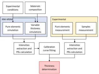
observations and historical information.
62
The approach described in this article differs from state of the art in the sense that we use
63
simulations to build calibration curves to determine the thickness of the coating. The same calibration
64
curve could be used for many samples instead of performing many simulations based on hypothesis.
65
This concept will be particularly interesting for industrial applications in metal deposition factories.
66
The simulations require a fast MC code, that is presently part of two software programs for such
67
application: XRMC [20] and XMI-MSIM [21,22]. Both codes use the Xraylib database [23]. XRMC is
68
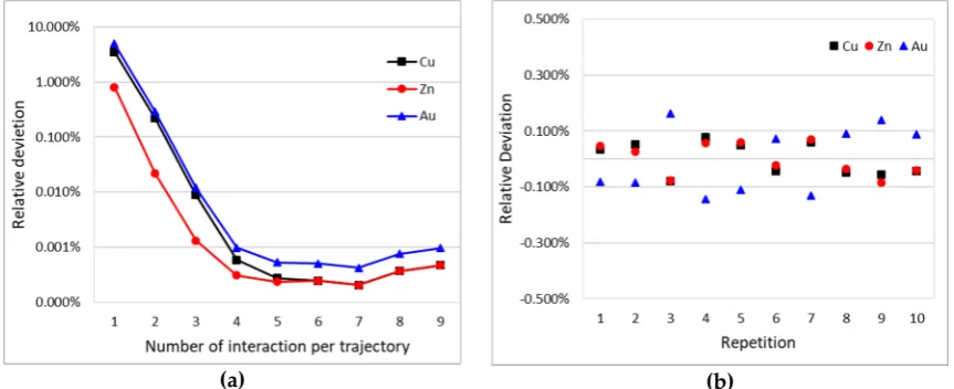
generally used for complex 3D geometries since XMI-MSIM can only simulate samples composed of
69
parallel layers. However, we decided to use XMI-MSIM because in our case the geometry is simple,
70
and this program is currently superior to XRMC in simulating XRF experiments [20]. XMI-MSIM is
71
the successor of MSIM, with a history of improvements of over 25 years [24–27].
72
In this work we examined a single layer sample of Au, Pd, Sn and white bronze on brass, using
73
both certified single element coatings and electroplated alloys. The results were compared with other
74
techniques for data validation: FP, FP + single empirical point and scanning electron microscopy
75
equipped with a focused ion beam (FIB-SEM). This is expected to provide an analytical method to
76
determine the thickness of coatings that does not make use of standards and whose performance is
77
comparable or even better to those of XRF analysis with energy dispersive (ED-XRF) systems on
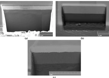
78
metallic coatings. Finally, we varied some parameters in the simulation to find out the ones that are
79
critical for the measurement and those that can be neglected to obtain reliable results.
80
2. Materials and Methods
81
The metal substrate consists of 3.75 x 5 mm brass (copper-zinc alloy) plates, 0.25 mm thick. The
82
substrate was electroplated with palladium and gold using a commercial galvanic bath “720 PDFE
83
MPM” and “8693 MUP” from Bluclad srl (Prato, Italy) and with white brass bath “SCUDO BIANCO
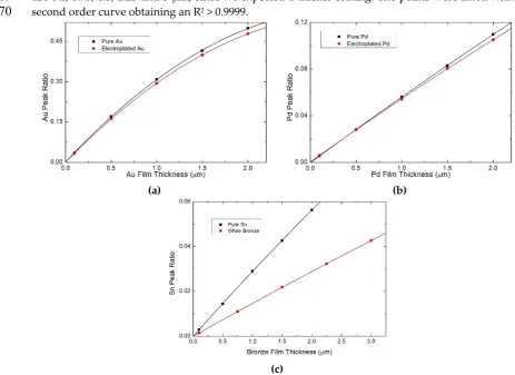
84
PLUS RACK” from MacDermid (Waterbury, CT, USA). The alloy composition and layer thickness of
85
the coatings are the subject of this study, and thus they will be discussed later. Certified samples with
86
known thickness are also used and were provided by Bowman (Schaumburg, IL, USA).
87
XRF measurements were performed with the Bowman B Series XRF spectrometer using an
88
acquisition time of 60 s, 50 kV tube voltage, 0.8 mA tube current and a collimator of 0.305 mm in
89
diameter. The same spectra were used to obtain the thickness information with various methods: FP,
90
FP with one empirical point correction (both available with the commercial software of the
91
instrument) and the MC method proposed in this study.
92
The composition of the substrate and the coatings were measured with energy dispersive X-ray
93
spectroscopy (EDS) microanalysis applying an accelerating voltage of 20 kV and scanning an area of
94
approximately 0.1 mm2 for a live time of 120 s. In order to consider the matrix effect, the ZAF
correction algorithm (atomic number, absorption and fluorescence) was used for quantification. For
96
this purpose, a gold-plated, a palladium plated, and a white bronze plated sample were prepared,
97
whose thicknesses were high enough to be considered infinite for the EDS analysis. The EDS analysis
98
was performed with a Hitachi (Tokyo, Japan) S-2300 equipped with a Thermo Scientific (Waltham,
99
MA, USA) Noran System 7 detector and analysed with Pathfinder software [28].
100
The SEM images and the FIB ablation were performed with a Tescan (Brno, Czech Republic)
101
GAIA 3 equipped with the Triglav electron column and the Gallium FIB Cobra Gallium column
102
XRF spectra simulations were performed with the open source software XMI-MSIM v7.0 64-bit
103
by Tom Schoonjans [21,22] which predicts the spectral response of ED-XRF using MC simulations.
104
The software allows setting many variables of the system under investigation as well as the hardware
105
geometry: this information was used as input to simulate the spectra.
106
The quantification method consisted of using the simulated spectra of 5 different layer
107
thicknesses to build a calibration curve, which was used to extrapolate the unknown thicknesses of
108
the measured samples. Simulations were performed using the exact composition of the coatings and
109
the substrates that were measured with EDS. The spectrum of each pure element of interest (Cu, Zn,
110
Pd, Sn and Au) was also both measured and simulated to obtain the relative intensity of the peak of
111
interest, called Peak Ratio (PR) henceforth. The PR concept is similar to the K-ratio used in the EDS
112
[29,30] and consists in the ratio between the peak intensity (X-ray counts) for the element of interest
113
in the sample and the peak intensity at the same energy for the pure element (equation 1).
114
𝑃𝑅
𝐼
𝐼
(1)XRF spectra were interpolated through multiple Gaussian [31–34] functions in the proximity of
115
the energy lines of the expected elements to obtain the peak area. The considered peaks were Cu Kα,
116
Zn Kα, Au Lα, Pd Kα and Sn Kα; in addition Cu Kβ and Zn Kβ were also fitted to avoid errors due
117
to peak overlaps. The PR were calculated, and the resulting data were fitted with a second order
118
curve. This kind of function is commonly implemented in XRF systems for industrial applications
119
since it is in good agreement with experimental data for a limited range of thicknesses and it is
120
moreover easy to manage. The complete quantification procedure is summarized in Figure 1.
121
122
3. Results
124
3.1. Software Validation
125
The applicability of the proposed method is strongly connected to the ability of the simulation
126
software to provide good results; for this reason, we evaluated the accuracy and the reproducibility
127
of XMI-MSIM.
128
A parameter that affects the accuracy of the simulations is the number of interactions per
129
trajectory: this number determines the maximum number of interactions that a photon can experience
130
during its trajectory. Low values bring to truncation errors, but too high values could result in a
131
computationally expensive simulation without any significant benefits in the results. Simulation of 1
132
μm of gold coating on brass was performed using values from 1 to 10 as the number of interactions;
133
the PR of each element for all the spectra was compared to the simulation with the highest number
134
of interactions permitted, and the relative deviation was calculated (Figure 2a). The results show an
135
exponential improvement for the first 4 interactions then, by increasing the number of interactions,
136
the deviation remains stable around 0.001 %: for this reason, all the following simulations were
137
performed using 4 interactions per trajectory.
138
The precision of the simulated spectra was evaluated repeating the same simulation on samples
139
consisting of 1 μm of gold on brass substrates 10 times. Then the deviation of the PR of each element
140
from the mean value was calculated (Figure 2b) as well as the relative standard deviation, that results
141
to be around 0.1 %.
142
After these tests, it can be concluded that the software results are good enough to allow its use
143
in the study and to proceed with the following experiments.
144
(a) (b)
Figure 2. PRs of Cu, Zn and Au of a simulated 1 μm of gold coating on brass substrates. (a) Relative
145
deviation of the PRs increasing the number of interactions respect to the simulation with 10
146
interactions; (b) relative deviation from the mean value repeating 10 times the same simulation.
147
3.2. Thickness Determination
148
After the preparation of the samples, they were measured with the XRF, then the spectra of
149
certified samples and the pure elements Au and Pd were collected. The FP method considers the
150
precious coating as pure for the thickness quantification. It was used both alone and combined with
151
a single empirical point. For the empirical point, the certified calibration standards were used. Then,
152
the thickness of the electroplated sample was measured with FIB-SEM performing a semi-destructive
153
(a) (b)
(c)
Figure 3. FIB-SEM images of the electroplated samples: (a) gold, (b) palladium and (c) white bronze.
155
A thick deposit of Au and Pd was electroplated separately (approximately 1.1 μm and 1.9 μm,
156
measured with XRF) and measured with EDS to find the actual composition (Table 1). The
157
composition of the certified thicknesses standards is known and is reported in Table 1 as well. The
158
results agree with the technical sheets of the baths; except the bronze that show a level of Sn higher
159
(47.2 %) than expected (28 – 35 %), this information will be useful in the determination of the
160
thickness.
161
Table 1. The composition of the substrate and the film investigated using EDS analysis.
162
Samples Electroplated Certified Brass
(substrate)
Cu: 63.0 wt% Zn: 37.0 wt%
Cu: 63.0 wt% Zn: 37.0 wt%
Au
Au: 97.9 wt% Fe: 1.6 wt% Ni: 0.5 wt%
Au: 100 wt%
Pd Pd: 95.2 wt%
Fe: 4.8 wt% Pd: 100 wt%
Bronze / Sn
Cu: 39.9 wt% Zn: 12.9 wt% Sn: 47.2 wt%
Sn: 100 wt%
Besides that, we performed the simulations with XMI-MSIM using the exact concentrations;
163
moreover, the intensities of the peaks were integrated using a multiple Gaussian peak fit. The spectra
164
of the pure elements Au and Pd were also simulated to obtain the PRs. Finally, we obtained six
165
calibration curves (Figure 4), each one containing 5 points corresponding to different thickness values
166
of the metal: for electroplated gold, certified gold, electroplated palladium, certified palladium and
167
use 0.1, 0.75, 1.5, 2.25 and 3 μm, since we expected a thicker coating. The points were fitted with a
169
second order curve obtaining an R2 > 0.9999.
170
(a) (b)
(c)
Figure 4. Calibration curves built from the simulations using the pure metals (black) and the
171
composition of the electroplated films (red) of (a) Au, (b) Pd and (c) Sn.
172
The peak intensities in the measured spectra were fitted with the same multiple Gaussian curves
173
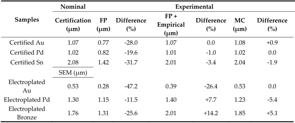
to calculate PRs values and finding the thickness of the samples. The results (Table 2) show a big
174
discrepancy in all the samples between the nominal value and the FP method; this deviation is highly
175
improved with the empirical correction. Keeping in mind that the certified samples were also used
176
as standards for the empirical correction, the good results obtained for the certified samples are not
177
very surprising; besides that, the result in the case of the electroplated samples are improved but still
178
with high accuracy error. On the other hand, the results obtained with the MC method are very
179
promising: the estimated difference is below 2 % in four out of six cases, and for two samples the
180
difference (0.0 %) is under the precision of the measurements. The case of electroplated palladium
181
and bronze the deviation is higher, around 5 %, but they are still better than the FP result. The causes
182
that produce these outliers will be studied in deep in the future, but we can advance hypotheses
183
based on what we observed during the quantification process. The Sn and Pd peaks are not very
184
intense, due to the characteristics of the samples and the detector, in these cases the signal to noise
185
ratio not very high, for the same reason also the matrix effect and the background subtraction are
186
important factors that must be taken in great consideration for accurate quantification.
187
The fitting of the calibration curve is good enough that if it is repeated by considering only 3
188
among the 5 simulated spectra, the variation will be only of approximately only ±0.3 %, meaning that,
189
in the case, this variation could be acceptable, the computational cost could be decreased
190
substantially. On the other hand, we found that the film composition influences the results strongly:
191
in Figure 4 there is an appreciable divergence, increasing the thickness, using pure metal coating
192
standards or the electrodeposited alloy, even if the composition varies only of few percental points.
193
If the pure standards were used for the quantification of the galvanic sample, the results would have
194
with the expected Sn concentration in the alloy was 35 %, it would have been 2.71 μm (54 % deviation
196
from the real value), for this reason, we performed the EDS analysis to obtain the exact composition.
197
Unfortunately, often it is assumed that the composition of the deposit does not change much over
198
time, leading to gross errors.
199
Table 2. Nominal (Certified and FIB-SEM) and measured (XRF) thickness calculated with FP and MC
200
methods for the samples.
201
Samples
Nominal Experimental
Certification (µm)
FP (µm)
Difference (%)
FP + Empirical
(µm)
Difference (%)
MC (µm)
Difference (%)
Certified Au 1.07 0.77 -28.0 1.07 0.0 1.08 +0.9
Certified Pd 1.02 0.82 -19.6 1.01 -1.0 1.02 0.0
Certified Sn 2.08 1.42 -31.7 2.01 -3.4 2.04 -1.9
SEM (μm) Electroplated
Au 0.53 0.28 -47.2 0.39 -26.4 0.53 0.0
Electroplated Pd 1.30 1.15 -11.5 1.40 +7.7 1.23 -5.4
Electroplated
Bronze 1.76 1.31 -25.6 2.01 +14.2 1.85 +5.1
3.3. Critical parameters of measurement
202
In the previous section, we proved the power of the MC method for thickness determination.
203
Then, more simulations were performed to predict the critical parameter that we need to take into
204
account when we measure a sample, regardless of the measurement method used.
205
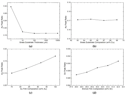
The first variable we considered was the thickness of the substrate: on too thin samples, the
X-206
rays could pass through giving a PR different from those expected. To investigate this phenomenon,
207
we simulated sandwich-like samples with 0.5 μm pure gold coating on both sides (to mimic a real
208
galvanic sample) and a brass layer in between, whose thickness ranged from only 1 μm up to 1 cm,
209
and we performed one simulation per order of magnitude. The influence of the thickness of brass
210
substrates is evident only for very thin dimensions (Figure 5a): over 0.1 mm, the difference to an
211
infinite bulk substrate is negligible, and the same calibration curve can be used for different samples.
212
Later, we investigated the influence of the alloy composition of both the coating and the
213
substrate on the PR. We examined typical deposits of common thickness used in galvanic industry:
214
0.5 μm gold coating alloy, 3 μm white bronze alloy and brass alloys. The expected variation in the PR
215
varying the composition of the alloys depends on secondary fluorescence and self-absorption of the
216
sample, which depends on the composition, meaning that for different elements the trend could be
217
different.
218
We investigated the influence of the brass composition on the Au PR. We simulated a 0.5 μm
219
pure gold coating on 1 cm brass substrate. Typical brasses are alloys of Cu and Zn in ratios ranging
220
from 62:38 (UNS alloy number C27200) to 70:30 (C26130) [35]. We simulated the following
221
concentration of Cu: 63 %, 65 %, 67 % and 69 %. In this range of concentration, the Au PRs does not
222
change significantly remaining in the error of the simulation (Figure 5b); the influence of the substrate
223
could be more remarkable for higher differences in the composition [36].
224
Then, the effect of the alloy composition of the coating was studied. First, we investigated the
225
Au-Cu alloy from pure gold to 18 kt (75 wt% Au) every 2 kt. As expected, the PR varies with the
226
concentration but, as also found for the electroplated gold with pure gold calibration curve, the
227
variation is bigger than the variation of gold concentration (Figure 5c); 22 kt gold (8.28 wt% Cu) gives
228
a value of -16.1 % with respect to the 24 kt while 18 kt gold (25 wt% Cu) gives -41.0 %. These findings
229
simply using a multiplicative factor even if the composition is known. For example, if an 18 kt gold
231
sample is measured and the thickness is estimated with a 24 kt curve to be 0.5 μm, we cannot affirm
232
that the actual thickness is 0.5 μm*24 kt/18 kt = 0.67 μm since this would underestimate much the
233
value.
234
The same study was carried out with a white bronze alloy on brass. The typical galvanic white
235
bronze composition is 50 – 55 wt% Cu, 28 – 32 wt% Sn, 14 – 20 wt% Sn. The calibration curve is
236
typically built using a standard of pure Sn, and the results are multiplied by 3.33 (assuming a 30 wt%
237
of Sn in the alloy). We simulated an alloy keeping fixed the amount of Zn at 17 % and varying the
238
concentration of Cu and Sn, using Sn concentrations from 28 wt% to 32 wt% every 1%. The simulated
239
sample consists of a 3 μm bronze layer, a 5 μm Cu layer and 1 cm of brass substrate: these thicknesses
240
and layer combinations are typical of nickel-free electrodeposition for wearable accessories. Also in
241
this case, similar to what we found for different alloys of gold, the composition plays a crucial role in
242
the thickness determination (Figure 5d) and the approximation, in this case, results in even worse
243
agreement: a variation of just 4 percentage points leads to an error of 12.2 %.
244
We also simulated a sample with 32 wt% Sn but with 10 μm of the underlying Cu layer, to see if
245
there would be any variation, but the thickness of the layer below didn’t seem to have any significant
246
influence.
247
(a) (b)
(c) (d)
Figure 5. Dependence of Au PR, of 0.5 μm gold film on brass simulation, (a) on the thickness of the
248
substrate, (b) on the composition of the substrate (expressed in percentage of Cu) and (c) on the
249
composition of the film, increasing the amount of Cu. (d) Dependence of Sn PR, of 3 μm bronze film
250
on brass, on the composition of the film, increasing the amount of Cu.
251
4. Conclusions
252
In the present work, we demonstrated the power of standardless MC calibration for measuring
253
the thickness of metallic coatings. We benchmarked the proposed method with the use of certified
254
standards and SEM imaging of FIB cross-sections. Our results indicate that the MC approach
255
metallic coatings in industry. Remarkably, this result was achieved without the use of a standard of
257
known thickness and composition.
258
The MC method has two major advantages: i) without the need of using standards allow an easy
259
switch between materials and coating architectures and ii) it can easily adapt to existing XRF
260
commercial systems as it requires only changes in the software.
261
After having validated the method and proved that the simulations give reliable results, we have
262
explored a few critical situations that may lead to major errors in the measurement both with the FP
263
and MC methods. We found that in the cases investigated, small variations in the composition and
264
the thickness of the substrate, or other eventual layers in multilayer architectures, don’t play a
265
substantial role on the PR of the element on the top. Conversely, the composition of the substrate
266
alloy must be exactly known; even a little deviation from the known composition can indeed bring
267
to large errors in thickness quantification.
268
In this work we have used the MC method to investigate the thickness limited to a single layer
269
on a substrate. In future, we will extend the technique to multilayer structures introducing a
270
multivariable approach. Such investigation is currently in progress.
271
Funding: This research was funded by Regione Toscana POR CreO FESR 2014-2020 – azione 1.1.5 sub-azione a1
272
Bando 2 “Progetti di ricerca e sviluppo delle MPMI” which made possible the project “Gioielli in Argento Da
273
Galvanica Ecologica e Tecnologica” (GADGET) and “Tecnologia al plasma per l’industria del lusso: una
274
manifattura innovativa nel comparto accessori in ottica 4.0” (THIN FASHION).
275
Acknowledgments: In this section you can acknowledge any support given which is not covered by the author
276
contribution or funding sections. This may include administrative and technical support, or donations in kind
277
(e.g., materials used for experiments). Bowman Coating Measurements Systems is gratefully acknowledged for
278
having provided technical information about the hardware and the internal geometry of the instrument. Authors
279
acknowledge Mr. Carlo Bartoli for the support given in keeping the FIB-SEM up and running.
280
Authors contribution: W.G. performed XRF measurements, MC simulations, data analysis and interpretation
281
and wrote the paper; E.B. performed part of the FIB SEM measurements; M.I. gave advice on the systems to be
282
investigated, on the electrodeposition of the materials and on paper revising; A.L. conceived the work,
283
supervised research, data analysis and paper writing.
284
Conflicts of Interest: The authors declare no conflict of interest.
285
References
286
1. Giurlani, W.; Zangari, G.; Gambinossi, F.; Passaponti, M.; Salvietti, E.; Di Benedetto, F.; Caporali, S.;
287
Innocenti, M. Electroplating for Decorative Applications: Recent Trends in Research and Development.
288
Coatings2018, 8, 260, doi:10.3390/coatings8080260.
289
2. Nygård, K.; Hämäläinen, K.; Manninen, S.; Jalas, P.; Ruottinen, J. P. Quantitative thickness determination
290
using x-ray fluorescence: Application to multiple layers. X-Ray Spectrom. 2004, 33, 354–359,
291
doi:10.1002/xrs.729.
292
3. Fiorini, C.; Gianoncelli, A.; Longoni, A.; Zaraga, F. Determination of the thickness of coatings by means of
293
a new XRF spectrometer. Arch. Intern. Med.1992, 152, 1969–1971, doi:10.1002/xrs.550.
294
4. Jalas, P.; Ruottinen, J.; Hemminki, S. XRF Analysis of jewelry using fully standardless fundamental
295
parameter approach. Gold Technol.2002, 35, 28–34.
296
5. Sitko, R. Quantitative X-ray fluorescence analysis of samples of less than “infinite thickness”: Difficulties
297
and possibilities. Spectrochim. Acta - Part B At. Spectrosc.2009, 64, 1161–1172, doi:10.1016/j.sab.2009.09.005.
298
6. Criss, J. W.; Birks, L. S. Calculation Methods for Fluorescent X-Ray Spectrometry: Empirical Coefficients
299
vs. Fundamental Parameters. Anal. Chem.1968, 40, 1080–1086, doi:10.1021/ac60263a023.
300
7. Kataoka, Y. Standardless x-ray fluorescence spectrometry (Fundamental Parameter Method using
301
Sensitivity Library). Rigaku J.1989, 6, 33–40.
302
8. Thomsen, V. Basic Fundamental Parameters in X-Ray Fluorescence. Spectroscopy2007, 22, 46–50.
303
9. Takahara, H. Thickness and composition analysis of thin film samples using FP method by XRF analysis.
304
Rigaku J.2017, 33, 17–21.
305
10. Han, X. Y.; Zhuo, S. J.; Shen, R. X.; Wang, P. L.; Ji, A. Comparison of the quantitative results corrected by
306
fundamental parameter method and difference calibration specimens in X-ray fluorescence spectrometry.
307
11. Pessanha, S.; Fonseca, C.; Santos, J. P.; Carvalho, M. L.; Dias, A. A. Comparison of standard-based and
309
standardless methods of quantification used in X-ray fluorescence analysis: Application to the exoskeleton
310
of clams. X-Ray Spectrom.2018, 47, 108–115, doi:10.1002/xrs.2819.
311
12. Vrielink, J. A. M.; Tiggelaar, R. M.; Gardeniers, J. G. E.; Lefferts, L. Applicability of X-ray fluorescence
312
spectroscopy as method to determine thickness and composition of stacks of metal thin films: A
313
comparison with imaging and profilometry. Thin Solid Films 2012, 520, 1740–1744,
314
doi:10.1016/j.tsf.2011.08.049.
315
13. Elam, W. T. T.; Shen, R. B.; Scruggs, B.; Nicolosi, J. Accuracy of Standardless FP Analysis of Bulk and Thin
316
Film Samples Using a New Atomic Database. Adv. X-ray Anal.2004, 47, 104–109.
317
14. Ager, F. J.; Ferretti, M.; Grilli, M. L.; Juanes, D.; Ortega-Feliu, I.; Respaldiza, M. A.; Roldán, C.; Scrivano, S.
318
Reconsidering the accuracy of X-ray fluorescence and ion beam based methods when used to measure the
319
thickness of ancient gildings. Spectrochim. Acta - Part B At. Spectrosc. 2017, 135, 42–47,
320
doi:10.1016/j.sab.2017.06.017.
321
15. Schiavon, N.; de Palmas, A.; Bulla, C.; Piga, G.; Brunetti, A. An Energy-Dispersive X-Ray Fluorescence
322
Spectrometry and Monte Carlo simulation study of Iron-Age Nuragic small bronzes (“Navicelle”) from
323
Sardinia, Italy. Spectrochim. Acta - Part B At. Spectrosc.2016, 123, 42–46, doi:10.1016/j.sab.2016.07.011.
324
16. Bottaini, C. E.; Brunetti, A.; Montero-Ruiz, I.; Valera, A.; Candeias, A.; Mirão, J. Use of Monte Carlo
325
Simulation as a Tool for the Nondestructive Energy Dispersive X-ray Fluorescence (ED-XRF) Spectroscopy
326
Analysis of Archaeological Copper-Based Artifacts from the Chalcolithic Site of Perdigões, Southern
327
Portugal. Appl. Spectrosc.2018, 72, 17–27, doi:10.1177/0003702817721934.
328
17. West, M.; Ellis, A. T.; Streli, C.; Vanhoof, C.; Wobrauschek, P. 2017 atomic spectrometry update-a review of
329
advances in X-ray fluorescence spectrometry and its special applications. J. Anal. At. Spectrom.2017, 32,
330
1629–1649, doi:10.1039/c7ja90035j.
331
18. Brunetti, A.; Fabian, J.; La Torre, C. W.; Schiavon, N. A combined XRF/Monte Carlo simulation study of
332
multilayered Peruvian metal artifacts from the tomb of the Priestess of Chornancap. Appl. Phys. A Mater.
333
Sci. Process.2016, 122, doi:10.1007/s00339-016-0096-6.
334
19. Barrea, R. A.; Bengió, S.; Derosa, P. A.; Mainardi, R. T. Absolute mass thickness determination of thin
335
samples by X-ray fluorescence analysis. Nucl. Instruments Methods Phys. Res. Sect. B Beam Interact. with
336
Mater. Atoms1998, 143, 561–568, doi:10.1016/S0168-583X(98)00412-1.
337
20. Golosio, B.; Schoonjans, T.; Brunetti, A.; Oliva, P.; Masala, G. L. Monte Carlo simulation of X-ray imaging
338
and spectroscopy experiments using quadric geometry and variance reduction techniques. Comput. Phys.
339
Commun.2014, 185, 1044–1052, doi:10.1016/j.cpc.2013.10.034.
340
21. Schoonjans, T.; Vincze, L.; Solé, V. A.; Sanchez Del Rio, M.; Brondeel, P.; Silversmit, G.; Appel, K.; Ferrero,
341
C. A general Monte Carlo simulation of energy dispersive X-ray fluorescence spectrometers - Part 5:
342
Polarized radiation, stratified samples, cascade effects, M-lines. Spectrochim. Acta - Part B At. Spectrosc.2012,
343
70, 10–23, doi:10.1016/j.sab.2012.03.011.
344
22. Schoonjans, T.; Solé, V. A.; Vincze, L.; Sanchez Del Rio, M.; Appel, K.; Ferrero, C. A general Monte Carlo
345
simulation of energy-dispersive X-ray fluorescence spectrometers - Part 6. Quantification through iterative
346
simulations. Spectrochim. Acta - Part B At. Spectrosc.2013, 82, 36–41, doi:10.1016/j.sab.2012.12.011.
347
23. Schoonjans, T.; Brunetti, A.; Golosio, B.; Sanchez Del Rio, M.; Solé, V. A.; Ferrero, C.; Vincze, L. The xraylib
348
library for X-ray-matter interactions. Recent developments. Spectrochim. Acta - Part B At. Spectrosc.2011, 66,
349
776–784, doi:10.1016/j.sab.2011.09.011.
350
24. Vincze, L.; Janssens, K.; Adams, F.; Jones, K. W. A general Monte Carlo simulation of energy-dispersive
X-351
ray fluorescence spectrometers-I. Unpolarized radiation, homogeneous samples. Spectrochim. Acta Part B
352
At. Spectrosc.1993, 48, 553–573, doi:10.1016/0584-8547(93)80060-8.
353
25. Vincze, L.; Janssens, K.; Adams, F.; Rivers, M. L.; Jones, K. W. A general Monte Carlo simulation of
ED-354
XRF spectrometers. II: Polarized monochromatic radiation, homogeneous samples. Spectrochim. Acta Part
355
B At. Spectrosc.1995, 50, 127–147, doi:10.1016/0584-8547(94)00124-E.
356
26. Vincze, L.; Janssens, K.; Adams, F.; Jones, K. W. A general Monte Carlo simulation of energy-dispersive
X-357
ray fluorescence spectrometers. Part 3. Polarized polychromatic radiation, homogeneous samples.
358
Spectrochim. Acta Part B At. Spectrosc.1995, 50, 1481–1500, doi:10.1016/0584-8547(95)01361-X.
359
27. Vincze, L.; Janssens, K.; Vekemans, B.; Adams, F. Monte Carlo simulation of X-ray fluorescence spectra:
360
Part 4. Photon scattering at high X-ray energies. Spectrochim. Acta Part B At. Spectrosc.1999, 54, 1711–1722,
361
28. Pathfinder Available online: https://www.thermofisher.com/order/catalog/product/
363
IQLAADGABKFAQOMBJE (accessed on Dec 20, 2018).
364
29. Raymond Casting Application of Electron Probes to Local Chemical and Crystallographic Analysis, 1951.
365
30. Giurlani, W.; Innocenti, M.; Lavacchi, A. X-ray Microanalysis of Precious Metal Thin Films: Thickness and
366
Composition Determination. Coatings2018, 8, 84, doi:10.3390/coatings8020084.
367
31. Watanabe, Y.; Kubozoe, T.; Mukoyama, T. Analytical functions for fitting K X-ray doublet peaks from Si(Li)
368
detectors. Nucl. Inst. Methods Phys. Res. B1986, 17, 81–85, doi:10.1016/0168-583X(86)90456-8.
369
32. McNelles, L. A.; Campbell, J. L. Analytic approximations to peak shapes produced by Ge(Li) and Si(Li)
370
spectrometers. Nucl. Instruments Methods1975, 127, 73–81, doi:10.1016/0029-554X(75)90304-3.
371
33. Van Espen, P.; Lemberge, P. Ed-Xrf Spectrum Evaluation and Quantitative Analysis Using Multivariate
372
and Nonlinear Techniques. Adv. X-ray Anal.2000, 43, 560–569.
373
34. Kikongi, P.; Salvas, J.; Gosselin, R. Curve-fitting regression: improving light element quantification with
374
XRF. X-Ray Spectrom.2017, 46, 347–355, doi:10.1002/xrs.2760.
375
35. Oberg, E.; Jones, F.; Horton, H.; Ryffel, H.; McCauley, C. Machinery’s Handbook; 30th ed.; 2016; ISBN
376
9780831130923.
377
36. Fan, Q. Simulation of relationships between substrate XRF intensities and film thicknesses. X-Ray Spectrom.