A serial optimization model for ranch management.

(1)

Literature Cited co. 1147 p.

Cook, C. Wayne, and Lorin E. Harris. 1968. Nutritive value of seasonal National Academy of Science. 1963. Nutrient requirements of beef cat- ranges. Agr. Exp. Sta. BuIl. 472. Utah State Univ., Logan. 55 p. tle. National Research Council. Pub. No. 1137. 32 p.

D’Aquino, Sandy A. 1972. Programming for optimum allocation of Sims, P. L., and A. H. Denham. 1969. Eastern Colorado Range Station resources: Eastern Colorado Range Station. PhD. Diss., Colo. State

Univ., Fort Collins. 244 p.

climatic data, 1956-1968. Prog. Rep. 6945, Agr. Exp. Sta., Colo- rado State Univ., Fort CoIlins. 3 p.

Farm Credit Bank of Wichita. 1969. Kansas City livestock prices Sims, P. L., G. R. Novell, and D. F. Hervey. 1971. Seasonal trends in 1959-69. Research Division, Wichita, Kansas.

Morrison, H. B. 1959. Feeds and feeding. Clinton, Iowa: Morrison Publ.

herbage and nutrient production of important sandhill grasses. J. Range Manage. 24:55-59.

A Serial

Optimization

Model

for Ranch

Management

E. T. BARTLETT, GARY R. EVANS, AND R. E. BEMENT

Highlight: A linear program resource management model is

described. This model is used to aid in the decision-making process of developing basic ranch management plans. A simple

one-year-at-a-time ranch management plan for the Central

Plains Experimental Range was developed. The model uses

discrete continuity equations to facilitate the flow of resources and products through seasons of the year. Management strate- gies based on the amount of initial operating capital ($20,000

to unlimited) are discussed.

Managers in business and industry are continually charged with making decisions concerning the efficient allocation of scarce resources. The economic existence of ranchers is based on efficiency. They must allocate their resources among alternative range products, such as cows and calves or yearlings, and must determine when and how best to use the resources. All these decisions affect economic resource allocation and are confounded by a myriad of alternative practices available to ranchers. It would be desirable to have a management technique that would compare alternatives and provide a quantitative guide for the rancher. Linear programming appears to be such a tool.

Linear programming is a mathematical optimization technique for allocating scarce or fixed resources to management alternatives. It consists of a set of linear equations which explicitly express, in mathematical terms, the limited resources, the management alternatives, and the decision-maker’s objective. Simply stated, “the objective in linear programming is to maximize or minimize a linear function subject to a number of linear constraints (Clough, 1963)“. The resulting optimum solution yields a set of computer decision guides for the resource manager to consider in relation to other nonquan-

The authors are assistant professor, Department of Range Science, Colorado State University, Fort Collins; range conservationist, U.S. Department of Agriculture, Soil Conservation Service and senior agency cooperator, Regional Systems Program, Colorado State University, Fort Collins; and range scientist, Agricultural Research Service, U.S. Dep. Agr., Fort Collins, Colorado.

This research is supported by NSF Grant No. G11333370 through the Regional Analysis of Grassland Environmental Systems Program at Colorado State University. RANGES Report No. 4 and Colorado State University Experiment Station (Scientific Series Number 18 34).

Manuscript received April 11, 197 3.

JOURNAL OF RANGE MANAGEMENT 27(3), May 1974 233

tified variables before selecting his final decision. Static linear programming models can only consider alternatives in a single time period. Serial linear programming models, as used in this paper, can consider an alternative in one time period in relation to an alternative in a previous time period. This relationship between static and serial models will be discussed in later sections of the paper.

This paper presents an example of how linear programming can be applied to ranching decisions and provides a guide to application in other resource management fields. In addition to static decisions in which all components are considered fixed, a serial linear model is presented which allows for seasonal growth of vegetation, the buying and selling of livestock, and cash flow of income and costs.

Dantzig (195 1) developed the linear programming technique shortly after World War II, and it was rapidly applied to problems in business. This method was successfully applied to agricultural problems before 1960 (Heady and Candler, 1958; Candler, 1956). Only during the past decade has linear programming been applied to natural resources. Nielsen and others (1966) used this technique in their study of federal range use and improvement for livestock production. Other workers developed models for multiple use of federal lands (Bell, 1970; Navon, 1967). D’Aquino (1972, 1974) developed a general resource allocation model using linear programming and applied this to a hypothetical ranching operation. D’Aquino’s model, however, was static with respect to the range resources. Consequently, if an acre of resource was used at one time, it could not be used again. The results of D’Aquino’s model and a serial model will be compared.

Study Area

Central Plains Experimental Range (CPER), totaling 15,700 acres, was used as an operating ranch. It is about 25 miles south of Cheyenne, Wyoming, and 12 miles northeast of Nunn, Colorado, in the central part of the Northern Great Plains shortgrass area. Annual precipitation ranges from 10 to 15 inches, with a summer (April-Sept.) mean of 10.17 inches and a winter mean (October-March) of 2.18 inches (Bertolin,

(2)

I

Subvector of Management Submatrix of Product Activitier I

I Activities

1

Submatrix Relating

I

Manegement Activities to Nul I

Fixed Resourcea

Submatrix I

I

Factors Required for _I Product Activitier Production aa Produced by :

Management Activities

Requirements for Factor8 of Production

Nul I Submatrix

I

I Identity Submetrlx

I Relating Productr to I Requirements

r

Subvector of 5

I

Fixed

I

Resovcer

Subvector of

> Minimum Leva Requl red ---- 1 Subvector of ->

_I

Pro&ct

L

Requirements

C

Subvector of Cortr I

I Subvector of Returns

1

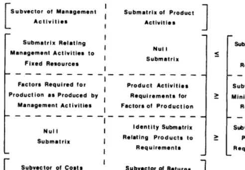
Fig. 1. Generalized structure of linear programming model of

D ‘Aquino (I 9 74).

level. Topography varies from nearly level to gently rolling hills with a fairly well-defined pattern. The soil series on the CPER have been mapped and described by the Soil Conserva- tion Service. These soil series were combined into groups based on common characteristics.

This grouping of soil series can be correlated with four distinct plant communities or range sites: Sandy Plains site, which includes 2,060 acres; Loamy Plains site with 11,099 acres; Overflow site with 2,020 acres; and Salt Meadow sites, which include 552 acres. Abandoned cropland, commonly called “go-back” land, takes 837 acres from the Loamy Plains site. Some of this will be considered for more intensive cropping.

Methodology

The resource allocation model developed by D’Aquino (1974) is shown in generalized form in Fig. 1. The model allocates the fixed resources among management alternatives. Factors of production or flow resources are generated from these fixed resources. These factors of production are used (consumed) by the product(s). In a ranch example, the fixed resources would be acres of rangeland, and the factors of production could include such items as pounds of forage dry matter and total plant protein. The salable product would be pounds of meat. This product, however, can be differentiated as to the animal that produces it: calf, lamb, or steer. The linear program maximizes the net revenue from the use of the resources. The results of the completely static model, as well as the results when the product prices are allowed to vary, are presented by D’Aquino (1974).

One weakness of the above model is that when an acre of a fixed resource is allocated in one management activity, it cannot be used in another. If, for example, the activities are forage use during different seasons, a particular acre of rangeland cannot be used during more than one season. This, at first glance, may not appear to be a major weakness; but if one season is a short use period during the spring the model cannot specify any use of regrowth in the fall if that area has already been allocated for spring use. A major objective of this study was to eliminate this weakness from the model. The magnitude of the problem can be demonstrated by examining one possible solution.

New management activities can be specified that represent all combinations of use, that is, spring use, spring-summer use, spring-fall use, spring-winter use, spring-summer-fall use, etc. The possible combinations are so numerous that the linear program rapidly becomes unwieldy. If, for example, all possible combinations for four seasons are considered, there will be fifteen management alternatives of use on each kind of rangeland. If the months of the year are considered as the

grazing seasons, the number of combinations increases to

4,095. In general, the number of possible uses is 2” - 1, where

n is the number of seasons.

Thus this method of alleviating the problem merely demonstrates the need for another method. The serial linear model described below alleviates the weakness while increasing the number of activities only to 2n - 1 instead of 2” - 1.

The continuity equation for a reservoir can serve as an example and is shown in equation (1) (Roefs, 1968).

St + I, - R, = St+i

(1)

Where S, is reservoir storage at the start of time period t, I, is the inflow during period t, and R is the release during period t. This relationship can rapidly be adapted to forage available at the start of any season. The continuity equation for usable forage can be written as

SC, + G, -

c, =

SC,,,

₍₂₎

Where SC, is standing crop at the start of period t, G, is growth during period t, C, is amount of forage used during season t, and SC,,, is the standing crop at the start of the next period.

Consider again the example of four seasons. The linear system of equations that results from applying equation (2) appears below.

SC,+G,-C,=SC, (3)

SC,+G,-C,=SC, SCa+G,-C3=SC, SC,+G,-C,>M

M is a minimum amount of forage that must be left on the range at the end of the grazing year, regardless of what date the computer selects as the time to terminate grazing for the year. Because SC, has been defined as usable crop, M is greater than or equal to zero. In this linear system, the standing crop at the start of season 1, growth during the four seasons, and the amount of forage to be left must be known. The other variables are decision variables whose values will be specified in the optimal solution. Such a linear system of equations can be formulated for each kind of rangeland on the ranch, and, together with rates of use by animal classes and the objective function (a linear equation relating costs of using resources and revenues of management alternatives), makes up a linear program.

The reservoir continuity equation (1) can also be applied to the flow of livestock during the year. The general equation is

Ht + Bt - St =Ht+1 (4)

where H, is the herd size at the start of season t, B, is the number of animals bought at the start of t, and St is the number sold at the end of period t.

The linear system for steers in a four-season year is shown in (5). In this system, the initial number of steers is the only required data.

Table 1. Approximate dates of grazing management periods.

Grazing period

1

2

3

4

5

Approximate date

May 16-June 30

July I-Aug. 31

Sept. I-Sept. 30

Oct. I-Oct. 31

Nov. l-May 15

Remarks

Temperature warm enough for

growth, if moisture available

Usual growth period, varies

with amount of precipitation

Forage dormant

Traditional sale period

(3)

H, +B, - S1 =H, (5) H,+B,-S,=H,

H,+B,-S,=H, H,+B,- S,>O

The values of the other variables are determined when these equations are placed in the linear model with the other constraints. The number of heifers that should be run on a ranch is described by a similar set of linear equations. It must be noted that the number of steers and/or heifers at the beginning of the year would be zero. The system of equations for a cow-calf alternative is slightly different from the linear system for steers (5). If it is assumed that calving occurs before or during grazing period one (Table 1 ), the system of equations is

H, - S, = H, (6)

H, - S, = H, H, - S, = H, H, - s4 > 0

H, specifies the initial calf-crop, and S, the number of calves sold at the end of season 1. Similarly, H, is the number of calves left at the start of season 2, S, is the number sold at the end of 2, and so forth. A similar linear system can be constructed for a ewe-lamb alternative. In the cow-calf and ewe-lamb alternatives, the cow and ewe must. be considered year-long. The development of brood stock requires a long- term capital investment (8-12 years) in relation to the short-term investment (6-8 months) for yearlings. A rancher usually has a minimum number of brood stock that he wants to run on the ranch. This minimum number may be specified in the initial grazing period. There are often instances, however, where the livestock producer is interested in finding out what the optimum number of livestock should be. The initial stocking rate then becomes a decision generated by the model.

Cash flow is also an important factor in ranch decisions. It can also be described in the fashion of equation (1).

-F

P

’ At Cit + Z rjt = At+1 (7)

i=l j=l

where At is the amount of cash available for investment at the m

start of season t, 2 Cit is the sum of the costs of m expen- i=l

P ditures during season t, and Z j=l

rjt represents the revenue from

p products sold during season t.

The linear systems for forage from each kind of rangeland, animal alternative, and cash were incorporated into the linear model of D’Aquino (1974) to form a serial linear programming model. The term serial is used to distinguish the above model from models using dynamic programming, another technique of operations research. A purely competitive market (for noneconomists this means that no single rancher can influence supply or demand by himself) and perfect knowledge (the assumption that the rancher is absolutely sure of all his production and market data) were assumed in the development and use of D’Aquino’s model and the serial linear model.

Application to CPER

Grazing management dates on the experimental area are based on functional management periods rather than on strict phenologic growth stages of the key forage species (Table 1). The frequent and unpredictable precipitation creates such erratic growth rates that reasonable management periods must

Table 2. !Seasonal forage production (lb) of kinds of rangeland.

Growth or loss

Season Loamy plains Sandy plains Overflow Salt meadow

1 + 39 + 39 + 28 + 40

2 + 304 + 542 + 380 +553

3 + 106 + 189 + 132 + 193

4 - 61 - 109 - 76 + 111

5 - 95 - 170 - 119 + 100

be based on plant growth stages combined with existing market conditions. Animal requirements are based on the average number of days in each management period.

Production data on available forage were extrapolated from biweekly production studies on Loamy Plains rangeland (Bement et al., 1965-71). Growth is based on the change in total standing biomass at the end of each previously described season and is shown in Table 2. Three hundred pounds of blue grama per acre on Loamy Plains will be left ungrazed at the end of the grazing season (Bement, 1969). Seasonal growth, total forage, and forage available for animal consumption were computed for each kind of rangeland. No seasonal production data were available for Sandy Plains and Overflow rangeland. Soil Conservation Service Range Site and Condition Guides, however, provide relative production values between various kinds of rangeland in the same Major Land Resource Area (Soil Conservation Service, 1970). The percent difference between median values of the Sandy Plains and Overflow rangeland was used for predicting growth and loss of forage on the sites. Forage growth and losses on the Overflow rangeland were assumed to be 20% greater than those on the Loamy Plains. Salt Meadow production averaged 50% greater than that of the Loamy Plains site. Checks at the end of the grazing season on the Salt Meadow site showed an average of 475 lb of forage remaining. Therefore, forage to be left at the end of the growing season on Salt Meadow rangeland was constrained to 475 lb/acre.

Data on nutrient availability in the range forage and supplements were obtained from Cook and Harris (1968) and Morrison (1959). Several assumptions regarding nutrient availability were necessary. It was assumed that species composi-

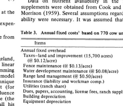
Table 3. Annual fixed costs’ based on 770 cow unit ranch.

Items Amounts ($)

Annual fixed overhead

Taxes-land and improvement (15,700 acres)

(@ $O.lIl/acre)

Fence maintenance (@ $O.l3/acre)

Water development maintenance (@ $O.O8/acre)

Range land management (@ $0.50/acre)

Insurance (liability and workman camp.)

Utilities (ranch share)

Dues, papers, accounting, license fees, ranch supplies

Building depreciation

Equipment depreciation

1,884.OO 2,041 .OO 1,400.00 7,850.OO 1,372.OO 1,292.oo 8,369.OO 1,338.OO 2,898.OO

Total $28,444.00

Annual livestock costs (per head basis)

Taxes

Veterinary expenses

Transportation

Commission and yardage

Labor

Truck and other equipment

Total

1.78 1.44 1.15 0.71 3.55 3.50

12.13

’ Based on Nelson and Skald (1970).

(4)

tion was dominated by three to four key species on each site. Species composition assumption was based on Hyder et al. (1966). Admittedly this omits consideration of many species; however, management must be based on the key or dominant vegetation occurring on a particular site or set of sites. The nutrient content of the species was based on Taylor (1972) and Morrison (1959).

The percent total nutrient content for the serial model was determined by a weighted calculation of the values of the percent composition of species and the nutrient content on a percentage basis. Nutrient values for dry matter, digestible protein, phosphorus, and carotene were calculated for each range site and each season. Digestible protein and phosphorus are computed on a pound-per-pound of dry matter basis, and carotene is calculated on a milligram per pound of dry matter basis. Nutrient content of the supplemental feeds considered were calculated from actual label tags of supplements currently being used for cattle on the experimental area.

It was assumed that all native range would be grazed in one or more of the five grazing seasons. The alternative of feeding alfalfa hay produced on up to 160 acres of irrigated alfalfa was considered. This alternative must also consider development of a center-pivot over-head sprinkler system, as well as production of the hay.

The only costs considered by the linear program are variable costs. Variable costs, in this paper, are those costs that vary directly in proportion to changes in productive output or activity and include annual irrigation system and hay production costs, supplement costs, purchase of livestock for resale, and maintenance of brood stock. When the management strategy has been developed, variable costs of each resource selected have been compared against the gross returns of the resource users. The resulting value is the contribution margin. Simply defined, contribution margin is the amount remaining after variable costs have been subtracted from gross revenue. Economists often refer to contribution margin as return to fixed factors, Fixed costs, as shown in Table 3, are then subtracted from the contribution margin to arrive at net income before taxes.

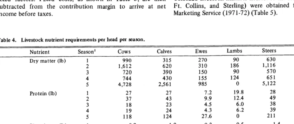
Table 4. Livestock nutrient requirements per head per season.

Annual cost of keeping the breeding cow, including bull cost and bull pasture charge, amounts to $47.54 per year with a 100% calf crop. Assuming a 90% calf crop, therefore, increases the annual cow cost to $52.82. The annual cost of keeping a ewe, including ram cost and ram pasture charge, is

$12.23. The annual yield of fleece is 8 lb, selling for approximately $21.00/cwt grease weight. This income can be deducted from the annual cost of the ewe, dropping the cost to $10.55. Assuming a 120-percent lamb crop at sale, the cost per ewe is reduced to $9.14.

The following classes of livestock were considered as user alternatives of the ranch resources:

1) Cow-calf - Cows would be bred to calve late in March, with weaning weight attained on October 1. However, calves may be sold in any season. Livestock requirements are based on the total nutrient requirement of both cow and calf (Table 4). Average gain of calf was 1.5 lb per day. Annual costs of cow and bull, and bull forage requirement, have been adjusted for a 90% calf crop.

2) Ewe-lamb - Ewes would be bred to lamb in March, with weaning weight attained on October 1. Average gain of the lamb was 0.5 lb per day. Annual costs of ewe and ram, and ram forage requirement, have been adjusted for a 120% lamb crop.

3) Steers - Steers may be bought at the start of any season or sold at the end of any season of the year. Nutrient requirements are adjusted for an average daily gain of 1.65 lb during the summer and 1 .O-lb daily gain during the winter.

4) Heifers - Heifers may be bought at the start of any season or sold at the end of any season of the year. Nutrient requirements are adjusted for 1.65 lb per day gain in the summer season 15 May-Ott 3 1, and 0.31 lb per day gain in the winter.

Because of the rapidly fluctuating livestock prices, it was assumed that the 1971-72 market prices would be most representative of the current market situation. Prices for the Colorado livestock markets nearest to the study area (Greeley, Ft. Collins, and Sterling) were obtained from Agricultural Marketing Service (197 l-72) (Table 5).

Nutrient Season’

Dry matter (lb) 1

2 3 4 5

Protein (lb) 1

2 3 4 5

Phosphorus (lb) 1

2 3 4 5

Carotene (mg) 1

2

3 4 5

I Seasons of the year defined in Table 1.

cows Calves Ewes Lambs Steers Heifers

990 315 270 90 630 675

1,612 620 310 186 1,116 1,178

720 390 150 90 570 570

744 430 155 124 651 651

4,728 2,561 985 0 5,122 4,334

27 27 7.2 19.8 28 39

37 43 9.9 12.4 49 52

18 23 4.5 6.0 38 40

19 24 4.3 6.2 39 42

118 124 27.6 0 211 100

0.9 1.8 0.3 0.5 1.4 1.4

1.2 2.5 0.4 0.5 1.9 1.9

0.6 1.2 0.2 0.2 0.9 0.9

3.9 7.9 1.2 0 3.9 3.9

4,320 765 76 356 1,260 1,350

5,952 1,054 105 490 1,736 1,860

2,880 510 69 237 1,320 1,440

2,976 527 87 74 1,364 1,488

(5)

Table 5. Average price from northeastern Colorado livestock markets (1971-1972).

Type Calves

Lambs

Heifers

Steers

Buying and

Weight selling

Date (lb) (S/cwt)

May 15, 1971 175 44.00

June 30, 1971 242 41.75

Aug. 31, 1971 335 39.50

Sept. 30, 1971 380 41.75

Oct. 31, 1971 426 35.75

May 15, 1971 58 10.00

June 30, 1971 72 12.50

Aug. 31, 1971 85 19.20

Sept. 30, 1971 96 20.10

Oct. 31, 1971 100 21.00

May 15, 1971 375 35.12

June 30, 1971 456 32.12

Aug. 31, 1971 568 32.25

Sept. 30, 1971 622 31.75

Oct. 31, 1971 678 33.00

May 15, 1972 739 31.50

May 15, 1971 375 38.88

June 30, 1971 456 37.12

Aug. 31, 1971 568 33.12

Sept. 30, 1971 622 34.38

Oct. 31, 1971 678 32.00

May 15, 1972 875 32.75

as salting with crushed salt and the increased labor cost may also be considered. A second group of alternatives for utilizing available forage or forage-producing areas may have been antelope and mule-deer, which have resident herds in the area, and other types of recreation which can utilize a range area. In an attempt to keep this management plan simple, only the major management alternatives were analyzed. The concept of linear programming is such that all alternatives to be considered are input at the same time and compared (mathe- matically) against each other to arrive at the best possible (optimum) mix for the particular operation being planned. This involves the application of simple cost and revenue analysis much more explicitly than has taken place in the ranch planning process. The cost of each unit of management input is identified by the decision maker during the initial planning phases.

The resulting management strategy would then be used by the decision maker as a guide to the development of the basic long-term management plan for his operation.

Discussion and Results

A management strategy consists of the basic fixed natural resources and other management and conservation alternatives allocated for optimum use by the resource users (livestock, wildlife, etc.). Should alternatives be left out or certain needs or desires of the rancher not be articulated on the initial run (solution derived by the computer) these can be changed and a second run or additional runs may be made until a satisfactory strategy is achieved.

Management alternatives other than those listed above To illustrate the above discussion, various management could also have been considered in this model. Alternatives strategies were derived from the simplified model of the CPER which contributed to additional available forage may have test ranch. The static deterministic model of D’Aquino (1974) been range pitting, contour furrowing, brush control, or a allocated the available grazing resources and supplemental feed combination of brush control and pitting. Other alternatives resources to provide a 12-month growing program for 653 may have been the development of additional stock water steers. All available forage was allocated at this level of facilities or cross-fencing for better distribution. Practices such stocking. Steers were purchased at the beginning of season 1,

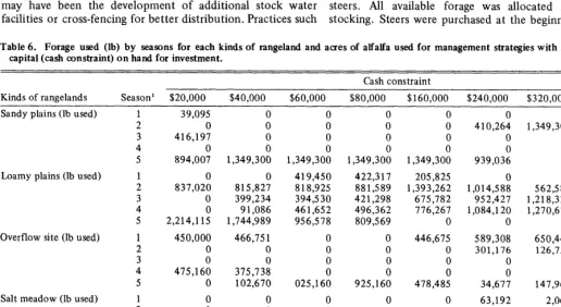
Table 6. Forage used (lb) by seasons for each kinds of rangeland and acres of alfalfa used for management strategies with varying amounts of capital (cash constraint) on hand for investment.

Kinds of rangelands

Cash constraint

Season’ $20,000 $40,000 $60,000 $80,000 $160,000 $240,000 $320,000 Unlimited-

Sandy plains (lb used) 1 39,095 0

2 0 0

3 416,197 0

4 0 0

5 894,007 1,349,300

Loamy plains (lb used) 1 0

2 837,020

3 0

4 0

5 2,214,115

Overflow site (lb used) 1 450,000

2 0

3 0

4 475,160

5 0

Salt meadow (lb used)

: 3 4 5

0 0 0 0 257,868 Alfalfa (acres used)

0 815,827 399,234 91,086 1,744,989 466,75 1

0 0 375,738 102,670 0 0 0 0 257,868

0 0 0 0 0

0 0 0 0

0 0 0 410,264

0 0 0 0

1,349,300 1,349,300 1,349,300 939,036

419,450 422,317 205,825 0

818,925 881,589 1,393,262 1,014,588

394,5 30 421,298 675,782 952,427

461,652 496,362

956,578 809,569

0 0

025,160 925,160

0 0 0 0 257,868

0 0 0

257,86:

0 626,458

1,349,300 722,842

0 0

562,588 1,313,290

1,218,325 1,619.352

776,267 1,084,120 1,270;670

0 0 0 1181493 0

446,675 589,308 650,440

0 301,176 126,752

0 0 0

478,485 34,677 147,968

0 63,192 2,060

0 194,676 255,808

0 0 0

257,868 0 0

0 0 0 5.11

0 0 0 0

0 0 0 17.77

3.75 5.24 6.14 50.66

0 0 0 0

0 0 0 925,160

0 0 257,868

0 0 0

’ Seasons of the year defined in Table 1.

(6)

carried through the entire year, and sold at the end of season 5, and 366 heifers were purchased at the start of season 1 and

istic model with the buying constraint. The parameter incre-

sold at the end of season 3, with a resulting contribution

mented was the operating capital available for investment at

margin (gross income less variable costs) of $97,3 12.18.

the start of period 1. The values of initial operating capital and the results are shown in Tables 6 and 7.

Available grazing resources and supplemental feed were allocated to create a management strategy calling for the livestock to be fed 326 tons of alfalfa hay from 160 acres of irrigated hayland on the ranch, and 2 tons of alfalfa pellets during season 1. The livestock would then be turned out to graze the range forage, with no supplemental feed during seasons 2, 3, and 4. As the quality of the range forage decreases during season 5, cattle would be fed protein supplement in the form of range cubes, cottonseed meal, and the remaining 79 tons of ranch-raised alfalfa.

At the initial value for operating capital ($20,000), a 374~0~ herd was indicated. The size of the cow herd steadily decreased as the amount of operating capital increased to $80,000. At $20,000 and $40,000, the calves were sold at the end of period 3, and money generated by the sale of the calves was then used to purchase yearlings for resale. As the amount of initial operating capital increased above $40,000, the number of cows stocked on the ranch dropped rapidly, since initial operating capital was now sufficient to start directly into yearling purchases.

The initial results from the serial model indicated a management strategy of grazing all the range during season 3 with 11,234 steers, resulting in a contribution margin of $270,677. Available forage was the first factor to become limiting. An implied limiting factor, however, is the impact that purchasing such a large number of animals in a short period of time would have on the market. Additional constraints were therefore added to the linear program so that not more than 500 head of steers and 500 head of heifers could be bought at the start of any one season. This initial run also showed that an unrealistic investment of more than $2 million would be required to carry out the mangement strategy.

A similar situation regarding lower levels of operating capital developed with the yearlings as the management strategy switched from cows to yearlings. Steers and heifers were bought at the beginning of a season and sold at the end of a season until $80,000 was available for investment. This was generating more investment capital for purchases in future seasons. As operating capital increased incrementally to $320,000, the management strategy approached that of the unconstrained capital situation, in which 500 steers and 500 heifers were purchased each season until season 3 and season 4, respectively, at which time they were sold.

The management strategy with the 500 head buying constraints, but with unlimited capital, was more realistic. At the start of season 1, 2, and 3, 500 head of steers were purchased; and at the start of 1, 2, 3, and 4, 500 head of heifers were purchased. Available forage was, again, the limiting factor. The steers were sold at the end of season 3, and the heifers at the end of season 4. A contribution margin

of $178,534.87 resulted from this management strategy. The strategy indicated that the manager required an initial operating capital of $490,605 in order to buy the animals. Allocation of the range and supplemental resources is shown in Table 6. Note that only alfalfa was used as a supplement (Table 6).

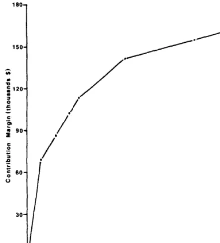
The contribution margin (gross income less variable costs) is shown in Figure 2. Marginal return to capital goes to zero at $490,605. This is not necessarily the optimal level of investment, because the manager’s alternative rate of return has not been considered.

Parametric runs (varying an input variable-parameter on each computer run) were then made, using the serial determin-

Available forage was a limiting factor in all runs. Protein became limiting only after the investment level was $160,000 or more, and as capital increased, protein became limiting in more seasons. Thus, the available range forage was fully utilized at all levels of investment and was used more efficiently as capital increased. Part of the reason that forage was used more efficiently was due to the fact that increasingly larger portions of the available forage were used earlier in the year, seasons 1, 2, 3,4, while forage quality was relatively high and less in season 5.

Table 7. Animal buying and selling strategies for varying amounts of initial available capital.

Initial operating capital limit

Variable Season’ $20,000 $40,000 $60,000 $80,000 $160,000 $240,000 $320,000 Unlimited

Calves sold (head) 3 374 254 61 0

5 .O 88 80

Steers purchased (head) 1 2 182 358 433 500 500 500 500

2 193 500 500 500

3 2 205 402 500 464 465 500 500

5 312 440 500 500 407 190 29

Steers sold (head) 1 2 182 358 433 500 334

2 193 666 863 0

3 2 205 402 462 464 465 637 1,500

5 312 440 500 538 407 190 29 0

Heifers purchased (head) 1 96 500 500 500 500

2 2 211 413 500 500 500 500 500

3 206 500 500

4 303 426 485 500 500 500 500 500

Heifers sold (head) 2 2 211 413 513 278

4 303 426 485 583 1,222 1,706 2,000 2,000

(7)

160

1

differen .t types 0 f livestock . It is therefore imperative that the market prices be predicted with greater precision than is now

150-

G

p” = 120-

: . /

1 _./

c ‘a _L a so-

I . /

S ._

5 /

0 .

._ _ 5 60- 0

0 I I I I I

0 60 120 160 240 320

Cash Available for Investment (thousands $1

Fig. 2. Marginal rate of return, as reflected by the

for each increment of available operating capital.

contribution margin

Conclusions and Recommendations

Ranchers and range scientists must efficiently allocate range resources and capital among alternative products. The serial model presented here provides a tool that enables managers to compare alternatives comprehensively. The use of the discrete continuity equation furnishes a valuable extension of D’Aquino’s allocation model, in that forage, animals, and cash are allowed to flow from season to season. In addition, it is not necessary to state explicitly all management and allocation alternatives; rather, a large number of alternatives are inherent in the flow equations.

The results of the parametric analysis showed the signifi- cant impact that the amount of cash available for investment has on management strategy. Not only do ranchers need to consider the efficient use of forage, but also the efficient use of their money. Not many ranchers currently consider the alternative of selling their calf crop early and buying yearling stock for resale. But, for individuals with limited cash, this may in fact result in maximum profit.

The model not only aids managers, it sheds important light on the development and application of future research needs. An important input into the serial model is the growth characteristics of range forage through the year. This type of information is scarce or nonexistent for most forage species. The management plan results, of course, depend on livestock prices and the relations that exist between the prices of

possible e

The current model is, of course, deterministic (assumed perfect knowledge of all variables). Future models should incorporate the stochastic (probabilistic) nature of rainfall and market prices and the dynamics of time that would enable the decision maker to implement a management strategy minimiz- ing the risk associated with predicting the future and planning operations for 3 to 6 years at a time.

Literature Cited

Agricultural Marketing Service. 1971. Livestock and Dressed Market

Report. Agr. Marketing Serv., U. S. Dep. Agr., Vol. LIV, Nos. 1243.

Bell, F. 1970. An example of optimization techniques in land

management: the Eldorado Model, p. 75-87. In D. A. Jameson (ed.),

Modelling and Systems Analysis in Science. Range Sci. Dep.,

Colorado State Univ., Fort Collins, Colorado. Sci. Ser. No. 5.

Bement, R. E. 1969. A stocking-rate guide for beef production on blue

grama range. J. Range Manage. 22:83-86.

Bement, R. E., W. R. Houston, and D. N. Hyder. 196571. Central

Plains Exp. Range Annual Reports. Agr. Res. Serv., U. S. Dep. Agr.,

Fort Collins, Colorado.

Bertolin, G. E. 1970. A climatology of the Pawnee National Grassland.

MS Thesis, Colorado State Univ., Fort Collins, Colorado. 76 p.

Candler, W. 1956. A modified simplex solution for linear programming

with varied capital restrictions. J. Farm Econ. 38:940-55.

Clough, D. J. 1963. Concepts in Management Science. Prentice-Hall,

Englewood-Cliffs, N. J. 425 p.

Cook, C. W., and L. E. Harris. 1968. Nutritive value of seasonal ranges.

Agr. Exp. Sta., Utah State Univ., Logan, Utah. Bull. 472. 55 p.

Dantzig, G. B. 1951. Maximization of a linear function of variables

subject to linear inequalities, p. 339-347. In T. C. Koopmans (ed.),

Activity Analysis of Production and Allocation. John Wiley and

Sons, Inc., New York.

D’Aquino, S. A. 1972. Programming for optimum allocation of

resources: Eastern Colorado Range Station. PhD Diss., Colorado

State Univ., Fort Collins, Colorado. 244 p.

D’Aquino, S. A. 1974. A case study for optimal allocation of range

resources. J. Range Manage. 27:228-233.

Heady, E. O., and W. Candler. 1958. Linear Programming Methods.

Iowa State Univ. Press, Ames, Iowa. 590 p.

Hyder, D. N., R. E. Bement, E. E. Remmenga, and C. Terwilliger, Jr.

1966. Vegetation-soils and vegetation-grazing relations from fre-

quency data. J. Range Manage. 19: 11-17.

Morrison, H. B. 1959. Feeds and feeding. Morrison Pub. Co., Clinton,

Iowa. 1147 p.

Navon, D. I. 1967. Computer-oriented systems for wildland manage-

ment. J. Forest. 65:473479.

Nelson, A. C., and M. D. Skald. 1970. Resources, costs, and returns on

cattle ranches in the mountain areas of Colorado by size of ranch.

Colorado State Univ. Exp. Sta. Tech. Bull. 101.45 p.

Neilsen, D. B., W. G. Brown, D. H. Gates, and T. R. Bunch. 1966. Eco-

nomics of federal range use and improvement for livestock produc-

tion. Oregon Agr. Exp. Sta. Tech. Bull. 92. 40 p.

Roefs, T. G. 1968. Reservoir management: the state of the art, IBM

Data Processing Division, Washington Scientific Center, Pub. No.

320-3508. 85 p.

Soil Conservation Service. 1970. Technical Guide. State Office, Soil

Conserv. Serv., U.S. Dep. Agr., Denver, Colorado. 300 p.

Taylor, J. 1972. Nutritive value of Colorado range plants. Ph.D. Diss.,

Colorado State Univ., Fort Collins, Colorado. 96 p.