Multiple Exposure Fusion for High Dynamic Range Image
Acquisition by PCA Based Algorithm.
Swati Dattatraya Pate.
Shreeyash College of Engineering and Technology, ME in Department of
Computer Science and Engineering, Dr. Babasaheb Ambedkar Marathwada University, Aurangabad (M.S.)
Abstract:-
Multiple exposure fusion means combination of multiple images taken with different exposures into a one single Image. In that input images are low dynamic range images and Resultant image is a high dynamic Range Image (HDRI).This is a common process for HDRI Acquisition. During this process, low and high exposures causes blackout and whiteout to some areas of the images, in which correspondence between the images is very difficult to find. More importantly, In Low Exposures, image creates noised images. These images are not clearly identified. To address this types problems this paper presents an accurate and efficient multiple exposure fusion method for the HDRI acquisition. We also proposed a weighting scheme and PCA based algorithm for the multiple image fusion .Our proposed method also solves the system for each colour channels. We also show that our method is superior as compared to the other conventional methods.
Index Term
s
-Multiple Exposure, High Dynamic range image (HDRI), Principle Component Analysis (PCA), Computer Graphics (CG).
1. INTRODUCTION –
In the application of Digital cameras and computer graphics, a High dynamic Range Images (HDRI) is widely used for high quality rendering with image based lighting. In the past days, to capture the High dynamic range images many methods have been proposed based on the
Multiple exposure principle. But most of the conventional methods have been failed since the intensities of the images are significantly different due to the failure of cameras response curve estimation. That methods does not solved the underexposure, overexposure and occlusion problems. In this paper we show that our method is superior as compared to reinhard global Operator
and Reinhard local operator methods. We used PCA based algorithm for image Fusion. The calculation of the real illumination is comparably easy (as long as the exposure times are known) there is an obstacle to overcome: Digital cameras map the perceived Algorithm and weighting Functions for image fusion.
2. MULTIPLE EXPOSURE FUSION
–
In photography, computer graphics and image processing exposure fusion is a technique for blending multiple exposures of the same scene into a single image. As in high dynamic range (HDRI or just HDR), the goal is to capture a scene with a higher dynamic range. The High dynamic range images (HDRI) are constructed by combining multiple images taken with different exposures. The input images having different exposure values. The resulting image will be more informative than any of the input images. In The exposures are set by changing shutter speeds. Here main purpose of our paper is to improve the accuracy of underexposed and overexposed regions.
In this paper we use weighting functions to discard saturated pixels, image sampling and tone HDR radiance mapping and luminance mapping. With the help of exposure matrix we solve system for each colour channels .finally we used PCA based algorithm for image fusion of previous method results to create our HDR image.
In the following sections, we introduce a technique for combining multiple exposure images for creating a HDR image. We show some weighting functions to overcome the problems of overexposed and overexposed region pixels.
2.1 Radiance Map
The radiance map is a presentation of the real illumination in a photographed scene. It can be created from a series of pictures with different exposure times taken from the exact same point of view.
2.2 Camera Response Function
Whilst illumination in a pixel to a discrete value. This mapping is, unfortunately, not performed linearly. Various factors, such as the sensor itself, the optical lens, the AD-Converter, add their own characteristics to the conversion. Rather than dealing with all factors by themselves we look for a function which governs all influencing factors. This function we call the 16Tcamera response function16T, or 16TCRF16T. Since the
CRF stays more or less the same through a series of pictures the easiest way to acquire it would be by some normative test pictures. If we know the real illumination for every pixel, the way from the measured illumination to the CRF is not far. But these pictures are hard to take. We need equipment to measure the exact brightness, have the necessary setup and then it also consumes time. Then when we change the camera, have an unknown camera or change our equipment (special lenses etc.) we have to do the whole procedure again. The rescue comes in the form of a famous method by Debevec, which he published for the SIGGRAPH 97. The idea is to discard the knowledge of the absolute brightness of the pixels and try to come up with a solution only using the photographs we already have.
The crucial equation comes on the form of:
Here 16TZRijR16T is the brightness of pixel i in the picture
j. 16Tf()16T is the CRF, 16TERiR16T is the real irradiance which was
measured, and 16TΔtRjR16T is the exposure time. We invert,
take the logarithm and come to:
We now want to find the function 16Tg()16T. Under the
assumption that 16Tg16T is monotonic and very smooth
we can transform this problem into a minimum least square set of equations. For this we randomly select a number of pixels. The exact setup can be found in the paper. Two additional points are worth noting: First, the pixels, which we choose for this equation system, should be noise-free. To achieve this we estimate the variance in the local neighborhood and reselect the pixel when it crosses a certain boundary. Second, also in the pictures we take we might run into under- and overexposure. Since we want to discard that information we scale the measured pixel values with a weight function. In our program different function were chosen to
optimize the results. In the Debevec paper a simple hat function was chosen.
2.3 Color
This process has to be done for all three color channels independently. The RGB for most cameras is slightly different in all colors. When we forced only one RGB to be used for all colors the color in the pictures was off. The final step, from the RGB and the taken pictures (which are LDR, for Low Dynamic Range), is pretty easy: We just sum over all the pictures for one pixel, multiplied with the corresponding exposure time and scale the result, using the RGB 16Tg16T which we calculated
before.
2.4 Weighting Function-
In our technique, the multiple exposure images are taken with different exposure time of a camera with other settings fixed. The images are combined to create the HDRI. In that weighting functions has small values for the underexposed and overexposed pixels, and these pixel values are ignored. Here in this paper we solves the ghosting problems. In this paper the weighting function is introduced because underexposed or overexposed regions are much less reliable than the regions of middle intensities .Thus in the conventional methods ,the weight is specified to be small for pixel values near saturation values 0 and 1 and high for the middle intensities. The role of the weight is to discard the saturated pixels .The region where the pixel values are close to 0 or 255 is backed up by other exposure with large weights.
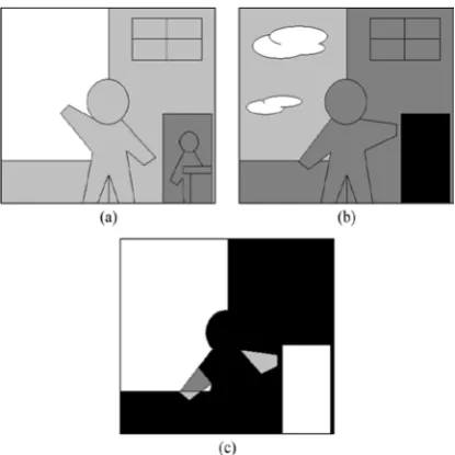
In conventional Methods, HDR images may fail due to occlusion, saturation that is underexposure and overexposure and differences in intensity caused by the failure of the camera response curve estimations. In our base paper following figure 1. shows an example of two exposures, where some part of high exposure image is overexposed [white region in (a)] and underexposed [black region in (b)].there may be three types of regions in high dynamic range images where correspondence between the images is difficult to find-1) marked by light grey (occlusion); 2)marked by white(saturation, overexposure);3) and both of the two.(dark grey).and noised images will be created because of failure in weights and Radiance map and camera response curve.
Fig. 1. Example of multiple exposure images: (a) high exposure, (b) low exposure,
(c) Occlusion (gray), and saturation (white).
2.5 Tone Mapping-
Creating HDR images usually requires a series of exposures of the same scene, then the following three steps are applied to compute a tone mapped version of the resulting HDR image: Recovering the camera response curve mapping real world brightness values to pixel values 0-255. Computing the HDR radiance map as a weighted sum from multiple exposures of the same scene. Compressing the contrast of the HDR radiance map while preserving details in order to display it on a non- HDR device (e.g. computer screen). This is called tone mapping. In order of being able to display a Radiance Map on a regular display it has to be compressed. The methods used are very much inspired by the human eye, since the goal is to achieve as natural an image as possible as a .na16Ttural16T is very subjective and mainly influenced
by the means with which the human eye adapts itself to different lighting conditions. All compression methods work in the 16Tluminance
domain16T and not in the often used 16TRGB domain16T. The
compression methods now want to accentuate areas which are dark, while very bright areas should be extenuated to ultimately create a homogenous illumination in the picture whilst lighting details should be preserved. The different compression methods are called 16Toperators16T and can be divided
into three main groups: Global, local and gradient domain based methods. In our project we chose to implement one operator from each group.
2.5.1 Reinhards Global Operator
A very simple yet effective operator is the global operator by Reinhard. Here the luminance values are scaled according to the average illumination throughout the whole picture. Bright areas are strongly dampened, while dark areas nearly stay the same. By normalizing afterwards an even level of illumination is achieved.
First we calculate the average log-illumination:
Here 16TN16T is the amount of pixels and 16TL(x, y)16T the
illumination of pixel at (x , y). To avoid calculating logarithm of zero we add δ. Next we try to estimate if the picture would be perceived as being bright or dark and call this estimator key of the scene. We scale the illumination for every pixel using the key and the averaged illumination:
Finally we now scale the luminance of every pixel:
For dark pixels this is nearly 1, whereas bright pixels are scaled with 1/L. After the reconversion into the RGB domain we normalize the picture.
2.5.2 Reinhards Local Operator
The local operator of Reinhard extends the mechanism of the global operator. The methods used for that are also known through analogous. Photography: Doging and Burning.. Here the development of the negative is manipulated to expose certain areas longer or shorter. By this, bright areas can be dialed down, while the contrast in dark areas can be improved. Over- and underexposed details can be made visible.
The first steps of the local operators are analogous to the global operator. Only the scaling of the luminance values of the pixels differs:
Here 16TVR1R16T is the luminance value blurred by a
Gaussian filter:
The challenge of the algorithm lies within the calculation of 16TsRmR16T from the formula above. For this,
Gaussian blurs of different magnitude are produced. Two neighbouring blurs are subtracted from each other as follows:
Finally all differences for one pixel are examined: If they are below a certain threshold 16TsRmR16T is chosen
accordingly.
3.PCA BASED IMAGE FUSION ALGORITHM-
PCA (Principle Component Analysis is widely used in image processing, especially in image compression.
Also, it iscalled the Karhunen-Leove transform KLT
or the Hotelling transform.This is a very simple inage fusion method. Principal components analysis PCA is
a statistical procedure that allows finding a reduced
number of dimensions that account for the maximum
possible amount of variance in the data matrix. The
PCA basis vectors are the eigenvector of the
covariance matrix of the input data.This is useful for
exploratory analysis of multivariate data as the new
dimensions called principal components PCs. A
reduced dimension can be formed by choosing the PCs associated with the highest eigenvalues. So, we
can consider KLT as a unique transform which
decorellates its input. Calculating a principal
components analysis isrelatively simple and depends
on some characteristics Associated with matrices eigenvalues and eigenvectors. To calculate the PCA we first estimate the correlation matrix or covariance
matrix of the image array. The next step is tocalculate
the eigenvalues of the matrix. Each eigenvalue can be interpreted as the variance associated with a single vector. The next step is to calculate the eigenvectors associated with each eigenvalue. Each eigenvector
represents thefactor loading associated with a specific
eigenvalue. By multiplying the eigenvector by the
square root of the eigenvalue. This is all the
information we need to begin to apply PCA. Finally,
we need to select the number of eigenvectors needed
to explain the majority data of the image. We simply
select the eigenvectors associated with the largest
eigenvalues to represent a sufficient amount of the image data.
3.1 PCA Algorithm-
Let the source images (images to be fused) be arranged in two-column vectors. The steps followed to project this data into a 2-D subspaces are: The most straightforward way to build a fused image of several input images is performing the fusion as a weighted superposition of all input images. The optimal weighting coefficients, with respect to information content and redundancy removal, can be determined by a principal component analysis (PCA) of all input intensities. By performing a PCA of the covariance matrix of input intensities, the weightings for each input image are obtained from the eigenvector corresponding to the largest eigenvalue. Arrange source images in two-column vector.
3.2 PCA
Advantages-PCA’s key advantages are listed below:
1) Reduced complexity in images grouping with the use of PCA.
2) Lack of redundancy
3) Smaller database representation since only the trainee images are stored in the form of their projections on a Reduced basis .
4) Reduction of noise since the maximum variation basis is chosen and so the small variations in the back-ground are ignored automatically.
4 .EXPERIMENTAL RESULTS:-
Following figure shows the results of our methods.-
(a)Image_1_1 (b) Image_1_2
(c) Image_1_4 (d) Image_1_6
(e) Image_1_8 (f) Image_1_12
(g) Image_1_15 (h) Image_1_30
(i)Image_1_120 (j)Image_1_250
(k)Image_1_2
(l)Image_1_2000
(m)Image_1_4000 (n)Image_15_1
(o) Image_4_1 (p) Image_2_1
Fig 2.sixteen Input images from (a-p) I1-I16.
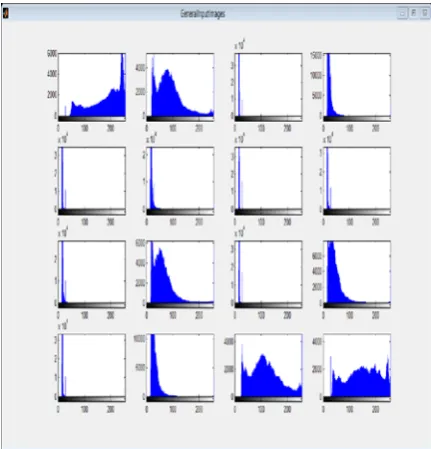
Next figure shows the all histograms of the input images.it is called as graphical representation of input images.
Fig.3.Histograms of input images
Following figure (fig 4.) shows the results of input images in Reinhard global operator and Reinhard local operator Methods.
. Fig.4.Result of Reinhard global operator and Reinhard local operator method.
Following Fig 5. Is the HDR image with histogram of input images of our method , Our result is clear and superior as compared to other previous methods.it overcomes the problems of occlusion and saturations .Our result is the average image of Reinhard global operator and Reinhard local operator methods .In that each region of image we can clearly identified.
Fig.5.Result of our method with Histograms.
5.CONCLUSION –
We have propose a technique for Multiple Exposure Fusion for high dynamic range images. In the method, we used PCA based image fusion to estimates the occlusion, saturation and noises in input images and constructs the HDRIs by removing artifacts. The proposed method
is superior to the conventional methods for most of the examples we have tested.
REFERENCES-
1) Takao Jinno, Student Member, IEEE, and Masahiro Okuda, Member, IEEE,” Multiple Exposure Fusion for High Dynamic Range Image Acquisition”, IEEE, Transaction image Process.vol.no.1.Jan.2012.
2) Reinhard , S. Pattanaik, G. Ward, and P. Debevec, High Dynamic Range Imaging: Acquisition, Display, and Image-Based Lighting, ser. Morgan Kaufmann Series in Computer Graphics and Geometric Modeling. San Mateo, CA: Morgan Kaufmann, 2004.
3) P. Debevec, “Image-based lighting,” IEEE Computer. Graph. Appl., vol.22, no. 2, pp. 26–34, Mar. 2002.
4) F. Mccollough, Complete Guide to High Dynamic Range Digital Photography.,China: Lark Books, 2008.
5) B. Hoe flinger, High-Dynamic-Range (HDR)
Vision, ser. Springer Series in Advanced
Microelectronics. New York: Springer-Verlag, 2006.
6) E. A. Khan, A. O. Akyuz, and E. Reinhard, “Ghost removal in high dynamic range images,” in Proc. IEEE Int. Conf. Image Process., Oct.2006, pp. 2005– 2008.
7) S. Mann and R. Picard, “On being ‘undigital’ with digital cameras: Extending dynamic range by combining differently exposed pictures,” in Proc. IS&T 46th Annu. Conf., May 1995, pp. 422–428.
8) A. G. Bors and I. Pitas, “Optical flow estimation and moving object segmentation based on median radial basis function network,” IEEE Trans. Image Process., vol. 7, no. 5, pp. 693–702, 1998.
9) E. Reinhard, M. Stark, P. Shirley, and J. Ferwerda, “Photographic tone reproduction for digital images,” ACM Trans. Graph., vol. 21, no. 3,pp. 267–276, Jul. 2002.
11) [Online]. Available: Http: //www.hdrsoft.com/P. E. Debevec and J. Malik, “Recovering high dynamic range radiance maps from photographs,” in Proc. SIGGRAPH, 1997, pp. 369–378.
12)http://cybertron.cg.tu-berlin.de/eitz/hdr/
Reinhard global operator
0 2000 4000
0 0.5 1
Reinhard local operator
0 2000 4000
0 0.5 1
HDR Image After Fusion
0 500 1000 1500 2000 2500 3000 3500 4000 4500 5000
0 0.5 1