Analysing Pattern for Chromium Bug Area
Classification
Trasha Gupta#, Monika Gupta* #Department of Computer Science,
Deen Dayal Upadhyaya College, University Of Delhi, Delhi, India
*Indraprastha Institute of Information Technology Delhi, India
Abstract— Software maintenance in software engineering is the modification of a software product after delivery to correct faults, to improve performance or other attributes. The purpose is to preserve the value of software over the time. The users report the bugs in the issue tracking system. Bug report contains many fields like title, description, version, OS, area etc. The quality of bug report affects the repair time. It is noticed that users often assign incorrect or don’t assign the area of bug which lead to bug reassignment and hence delay. Document categorization (based on text) with its diversified application has been widely studied by data mining, machine learning, and information retrieval communities. In this work we analyse the linguistic patterns to classify the bug into most three common areas: UI, web-kit and internals. The data set will be categorized using different classifiers viz. Naive Bayes, Support Vector Machine and Neural Networks etc.
Keywords— Text classification, area prediction.
I. INTRODUCTION
A. Motivation
Quality of bug reports submitted to defect tracking systems is a topic that has attracted a lot of research attention. Previous studies reveals that the quality of information present in a bug report influences its resolution time and has impact on the productivity of the development team. Better the quality of bug report, lesser will be the fixing time. Area identification can help in proper bug assignment so as to avoid delay due to reassignment. The choice of textual data to grab this valuable information has a very intuitive reason at its core. While writing a bug report, the reporter, though himself not aware of the actual reason, tries to replicate the situation in which the error occurred. This replication contains sufficient evidences for a trigger or bug-fixer to identify the area of bug. So, this work aims at grabbing this intuitive power to automate the area assignment
B. Problem Description
The textual data (label followed by attributes) of a bug report is served as input to different classifiers. These classifiers build a model to correctly classify the area of bug reports. The performance of the various techniques are evaluated and compared.
II. BACKGROUND
Text categorization is the task of assigning a Boolean value to each pair < dj, ci > ϵ D
×
C, where D is a domain ofdocuments and C = {c1,..., c|C|} is a set of predefined categories. A value of T assigned to < dj, ci >
ϵ D
×
C indicates a decision to file dj under ci, while a value of F indicates a decision not to file dj under ci. More formally, the task is to approximate the unknown target function, S': D×
C → {T, F} by means of a function S: D
×
C → {T, F} calledthe classifier (aka rule, or hypothesis, or model) such that S' and S coincide as much as possible.
So given a test instance, we wish to predict a class label using the training model. The classification problem can be seen broadly in the following two versions: hard version and soft version. In hard version, a class label is explicitly assigned to the problem, whereas in soft version, a probability value is assigned to the test version. Other variations include assigning rank to different class choices.
The classification problem assumes categorical class labels, though continuous labels (regression modeling problem) are also possible. Broadly text classification problem can be viewed as a set-valued feature, where the presence or absence of a word predicts the class label. However, in practice the relevance of a term plays a very vital role where the relevance can be described in terms of the frequency of occurrence of terms. Thus, a text classification can be described by the sparseness of the word attributes and high dimensionality. The text classification technique can be divided into two heads: discriminative classifiers and generative classifiers. Some methods which are commonly used for text classification are:
Decision Tree: It constructs a hierarchical division of the
underlying data space with the use of different text features
Pattern (Rule)-based: This classifier constructs a set of
rules based on word patterns which are most likely related to the different classes.
SVM Classifier: It determines optimal boundaries (linear or
nonlinear) between different classes [2].
Neural Network Classifier: It adapt to the use of word
features [4].
Bayesian (Generative) Classifiers: These classifiers
attempt to build a probabilistic classifier based on modeling the underlying features in different classes [3].
Feature selection is an important problem for text classification. In this we attempt to determine the features that are most relevant to the classification task. The measures such as gini index or the entropy are used to determine the level to which the presence of a particular feature skews the class distribution.
C. Feature Selection for Text Classification
The most fundamental task before classification is document selection and feature selection. Its importance, particularly in text data is due to the high dimensional text features and irrelevant features (noise). In general, a text can be represented as: bagofwords and textrepresentation as string. However, for simplicity, most text classification methods use bag-of-words model.
Most commonly applied techniques for both supervised and non-supervised applications are stop-word removal and stemming. In stop-word removal, the words which are not specific or discriminatory to different classes are eliminated. While in Stemming, different forms of the same word are consolidated to one.
III.METHODOLOGY
A. Naive Bayes Classifier
Naive Bayes is the simplest and commonly used generative classifier. It models the distribution of the documents in each class using a probabilistic model with independence assumption. These models compute the posterior probability with ”bag of words” assumption. Naive Bayes Classification is a token based approach to text classification. For a given character sequence, it returns the joint probability estimates of categories and tokens.
P (category|text) = P (text|category) * P (category)/P (text) Where P (category) is the prior probability of occurrence. The naive property about Naive Bayes is that it assumes a ”bag of word” model. In this model, all terms are considered independent of each other. Thus, a text can be visualized as a sequence of tokens, where all the tokens are independent of each other i.e.
The above equation can be written as:
The conditional probability P(category|terms) is defined in terms of two values: P(tokenjcategory) and P(category). We follow a step-by-step algorithmic procedure to construct a Naive Bayes Classifier for text classification [1]. The process is defined as
1. Data Extraction 2. Preprocess 3. Train 4. Test/Evaluate
B. Data Extraction
The size of the chromium bug report dataset as observed on the day of data extraction was approximately 1.8 lakh. From this whole, the reports for which area = UI or Internals or Webkit were selected for evaluation. The count of these
reports is 67546. The chromium dataset is labeled, with 25017 classified as UI bug-reports, 26,808 as Internals and the remaining (15724) as webkit bug report. The training/testing data is divided in the ratio of 80/20 (i.e., 13511 for testing and rest for training). This dataset is provided to the Classifier for further computations.
C. Preprocess
Each file in the train/test set is tokenized by using a wrapping TokenizerFactory, which converts character sequences into sequences of token. The resultant is feed to the Regular Expression filter which extracts only alphanumeric sequences, thereby eliminating any special character sequence. All the tokens are converted to their lowercase equivalent. Finally, all the stop words including preposition, conjunction etc. are removed from the set of tokens. This task is achieved using the following code.
D. Train
Traditional Naive Bayes uses maximum a posterior (MAP) estimate of the multinomial distribution. Dirichlet smoothing is incorporated by adding a fixed prior to each count in the training data. Two counts are used to estimate the parameters:
tokencount(w,c): number of times token w occurs in the training set for category c.
casecount(c): number of training instances for category c.
The prior probabilities of casecount and tokencount are supplied through constructors to the classifier. So,
The model is trained on various values of supervised dataset.
E. Evaluate
The trained model is provided to the test dataset, which then evaluates it using various performance measures.
F. Expectation Maximisation in Lingpipe’s Naive Bayes EM works by iteratively training better and better classifiers using the previous classifier to label unlabelled data to use for training.
G. SVM Classifiers
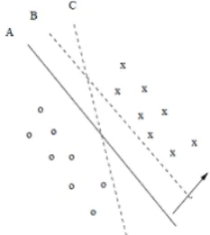
SVM is a linear classifier for which the output
is a separating hyper-plane between the two classes. The hyper-plane specifies the maximum margin of separation. It is closely related to feature transformation methods, such as Fisher discriminant. It has been observed that text data is ideally suited for SVM classification because of the sparse high-dimensional nature of text.
Fig 1: What is the best separating hyperplane?
It is not necessary to use linear function for SVM classification. By using the kernel trick, one can construct a non-linear decision surface by mapping the data instance non-linearly to an inner product space where the classes can be separated linearly by a hyper-plane.
H. Neural Networks
Fig 2: Multi-layer neural network for nonlinear separation
The basic unit in a neural network is a neuron or a node. The input to the system is the term frequencies of the ith document. A neural network is an interconnection of these nodes where the connecting edge carries some weight. Thus a typical linear function used in neural network is as follows:
To induce complex, non-linear decision boundaries, multiple layer neural networks are used. The training process is quite complex and error needs to be back-propagated over different layers.
I. Performance Evaluation
Classic IR notions for effectiveness are Precision (π) and Recall (ρ). Precision for a class ci is defined as a conditional
probability
i.e. if a random document is classified under ci, then the
decision is correct. Analogously, recall for a class ci is
defined as
i.e. if a random document dx ought to be classified under
ci , this decision is taken. These probabilities can be
False Positive (FPi) True Positive (TPi) False Negative (FNi) True Negative (TNi)
Other Measures can be accuracy, error, F-measure etc. The cumulative match curve (CMC) is used as a measure of 1:m identification system performance. It judges the ranking capabilities of an identification system. The Receiver Operating Characteristic (ROC) is used as a measure of verification system performance.
IV.CHOICE OF TECHNIQUE
Broadly the classifiers can be divided into two heads: Generative Classifiers and Discriminative Classifiers
A. Generative Classifier
Bayesian Classifier: Multinomial Bernoulli Model is chosen.
B. Discriminative Classifier
SVM: linear/non-linear decision boundary with feature transformation
Neural: multilayer back propagation neural network
K-Nearest Neighbour: Object classified by majority vote of its neighbours.
V. ANALYSIS OF DATASET
Data of Google chromium issue tracking system is chosen for analysis. It finds its roots in the problem statement of automated bug classification. A bug report is a semi-structured text, with different attributes cumulatively conveying information about a single bug report. Above 1 lac Bugs were extracted for 4 years. A subset was chosen for an approximately 65K bugs belonging to UI, webkit and build are extracted for the classifier design. Training and Testing data Approximately 50 K used for training and remaining 15 K for testing.
Here we are looking for the textual aspect of bug interpretation to find distinguishing features for classification. Following is the list of attributes identified in a typical bug report extracted from a Chromium data set.
IssueIDA: unique identifier for each bug report
State: Closed or Open.
Status: Fixed, Duplicate, and Verified
Reported Time-Stamp: The starting and closing
time of a bug
Reporter: The person who reported the bug
owner: The person who is assigned the bug
Title: The label of the bug
Description: Long description of the bug
Area: The intuitive area of bug. It can have values:
UI, internals, webkit, build, compat, chrome frame etc.
Type: The nature of bug. It can be Bug, Feature,
Regression, Usability, Localization, Polish, Other, Security, Task, Clean-up, Meta, Test, Documentation, Defect, Feature Tracker, Yak
Priority: 0,1,2,3
Length of Description: Total length of the
description
Operating System: The operating system on which
bug is observed.
Since here we are looking for the textual aspect of bug interpretation along with some discrete features, so the attributes of concern are:
Title Description Operating System
VI.RESULTS
TABLE 1:NAIVE BAYES RESULTS
Case Accuracy (%) Recall (%) Precision (%) F(1) (%) Full
Evaluation 66 63.85 70.59 66.07
Internals Vs
All 74.9 59.9 72.1 65.4
Webkit Vs
All 85.1 46.9 81.0 59.5
UI Vs All 72.1 84.6 58.5 69.2
TABLE 2:CONFUSION MATRIX FOR NAIVE BAYES RESULTS
Reference Vs Response Internals Webkit UI
Internals 3212 221 1929
Webkit 597 1478 1070
UI 643 124 4237
TABLE 3:10-CROSS FOLD RESULTS FOR NAIVE BAYES
Average 77.3%
TABLE 4:EM IN LINGPIPE’SNAIVE BAYES
Average 63%
TABLE 5:SVM RESULTS
Kernel Function Linear(best) Accuracy 79.73%
TABLE 6:CONFUSION MATRIX FOR SVM (LINEAR KERNEL)
Reference Vs
Response UI Internals Webkit
UI 2494 2106 0
Internals 0 5362 0
Webkit 98 374 2672
TABLE 7:RESULTS FOR SVM (LINEAR KERNEL),ONE VS ALL
Case Precision (%) False Positive
Internals Vs All 100 0
Webkit Vs All 85.0 15
TABLE 8:K-NN RESULTS AT K=10(BEST)
REFERENCES
[1] Sureka, Learning to Classify Bug Reports into Components, 50th International Conference on Objects, Models, Components, Patterns (TOOLS Europe), 2012
[2] http://svmlight.joachims.org/
[3] http://en.wikipedia.org/wiki/Naive_Bayes_classifier [4] http://en.wikipedia.org/wiki/Artificial_neural_network
Accuracy 10-Fold average accuracy
78.5 73.76
No. Of Layers 3
No. Hidden Nodes 10, 20
No. Of nodes for best
results 10