Side-Channel Leakage and Trace Compression using Normalized Inter-Class Variance

Side-Channel Leakage and Trace Compression

using

Normalized Inter-Class Variance

Shivam Bhasin

_{, Jean-Luc Danger}

_,

Sylvain Guilley

_{and Zakaria Najm}

1

_{Institut MINES-TELECOM, TELECOM ParisTech,}

CNRS LTCI (UMR 5141),

Department COMELEC, 46 rue Barrault,

75 634 PARIS Cedex 13, FRANCE.

2

_{Secure-IC S.A.S., 80 avenue des Buttes de Co¨esmes,}

35 700 Rennes, FRANCE.

Abstract

Security and safety critical devices must undergo penetration test-ing includtest-ing Side-Channel Attacks (SCA) before certification. SCA are powerful and easy to mount but often need huge computation power, es-pecially in the presence of countermeasures. Few efforts have been done to reduce the computation complexity of SCA by selecting a small sub-set of points where leakage prevails. In this paper, we propose a method to detect relevant leakage points in side-channel traces. The method is based on Normalized Inter-Class Variance (NICV). A key advantage of NICV over state-of-the-art is that NICV does neither need a clone de-vice nor the knowledge of secret parameters of the crypto-system. NICV has a low computation requirement and it detects leakage using public information like input plaintexts or output ciphertexts only. It is shown that NICV can be related to Pearson correlation and signal to noise ratio (SNR) which are standard metrics. NICV can be used to theoretically compute the minimum number of traces required to attack an implemen-tation. A theoretical rationale of NICV with some practical application on real crypto-systems are provided to support our claims.

1

Introduction

Security-critical devices must undergo a certification process before being launched into the public market. One of the many security vulnerabilities tested in the certification process is Side-Channel Attacks (SCA [4,5]). SCA pose a serious practical threat to physical implementation of secure devices by exploiting un-intentional leakage from a device like the power consumption, electromagnetic emanation or timing. Several certification/evaluation labs are running SCA daily on devices under test to verify their robustness.

The certification process is expensive and time-consuming which also in-creases the overall time-to-market for the device under test. It worsens when the desired security level increases. For instance, it is usually considered that a Common Criteria (CC [7]) evaluation at highest assurance level for penetra-tion attacks (AVA.VLAN.5) requires the device to resist attacks with 1 million traces. Similarly, the draft ISO standard 17,825 [12] (application note for in-ternational standard ISO/IEC 19 790, sibling to NIST / FIPS 140-2) demands resistance against side-channel analysis with 10,000 traces (level 3) and with 100,000 traces (level 4). The traces can have millions of points and thus run-ning SCA on these traces can be really time consuming. Also several attacks must be tested on the same set of traces before certifying a device. To accelerate the evaluation process, a methodology should be deployed which compresses the enormous traces to a small set of relevant points.

1.1

Related Works

The compression of SCA traces which results in reduced time complexity of the attacks, can be achieved by selecting a small subset of points where leakage prevails. This issue of selecting relevant time samples have been dealt previously by some researchers. Chari et al. [5] use templates to spot interesting time samples. The method involves building templatesT onndifferent values of the subkey. Interesting time samples can then be found as points which maximizes Pn

i,j=1(Ti −Tj). In this equation, Ti is the average of the traces when the

sensitive variable belongs to the classi. Two further improvements were then proposed by Gierlichs et al. [14]. The first improvement, also called as Sum Of Squared pairwise Differences (SOSD), simply computesPn_i,j=1(Ti−Tj)2. SOSD

avoids cancellation of positive and negative differences. SOSD can be further improved by normalizing it by some variance. This normalized SOSD is called SOST (Sum Of Squared pairwise T-differences [14], where aT-differencemeans aStudent T-test) and computed as

n

X

i,j=1 

 Ti−Tj

q

σi2

mi +

σj2

mj   2

, (1)

whereσiis the variance ofT in classi, andmiis the number of samples in class

times the estimated probability for the traces to belong to classi. When the classes are equally populated (i.e.,_∀i, mi=m/n), the SOST rewrites as:

m n

n

X

i,j=1

(Ti−Tj)

2

σi2+σj2

,

Similar ideas were also sketched earlier in [9].

A practical problem with template-based detection techniques comes from the computation of templates. First of all, templates require an access to a clone device. Secondly, templates need two sets of traces: one for profiling with random keys and another for attacking with an unknown but fixed key. An alternative to the latter limitation is model-based templates which can exploit the same set of traces as proposed in [1]. Although model-based templates can be really efficient, they are relevant for the chosen power model only.

Another method proposed in this context is the Principal Components Anal-ysis (PCA [20]). PCA is used for dimensionality reduction. It yields a new basis of the time samples in which the inter-class variance is greater. This basis takes into account the covariance of the samples. In side-channel analysis, the goal of PCA is to gather all the information in a single (or few) component(s) [2]. Eventually, other empirical methods use chosen plaintext attacks, such as the differences between plaintexts 0x00. . .0000 and 0x00. . .00ff. This technique requires many requests to check for all the bytes, not only the least significant byte. Furthermore, it is not always possible to choose the plaintext messages (e.g., when modes of operations with initial vectors are used).

In this paper, we propose a new method for leakage detection relying on a metric called “Normalized Inter-Class Variance” (NICV). This NICV method allows to detect interesting time samples, without the need of a profiling stage on a clone device. Hence the SCA traces can be compressed and the analysis could be greatly accelerated. The main characteristics of the proposed method are:

• NICV operates without the need of a clone device, i.e., it requires no profiling stage and use the same set of traces which are to be analyzed,

• it uses only public information like plaintext or ciphertext,

• the method is leakage model agnostic, it is not an analysis tool but a helper to speed up the analysis, but

• it can serve to evaluate the accuracy of various leakage models and choose which is the best applicable.

Compared to PCA, the purpose of NICV is to return the total variation of the traces at each time sample, so as to test which leakage model causes inter-class variation.

NICV with existing side-channel metrics like Pearson Correlation Coeffi-cient and Signal to Noise Ratio (SNR). NICV is also compared against other leakage detection techniques like SOST and SOSD. Secondly, we provide the theoretical lower bound of number of traces to recover the key. Finally, we apply NICV to real implementations on FPGA and smartcards to show its ability of leakage detection and other related applications.

The rest of the paper is organized as follows. General background to SCA is recalled in Sec.2. The rationale of NICV to select SCA relevant time samples is detailed in Sec.3. We also derive in this section a lower bound on the number of traces to recover the key. This is followed by some practical use cases applied on real devices like FPGA and smartcards in Sec.4. Finally, Sec.5 draws general conclusions. In appendixA, we provide with a comparison between NICV and TVLA (Test Vector Leakage Analysis [15]), two leakage detection metrics.

2

General Background

Side-channel analysis consists in exploiting dependencies between the manip-ulated data and the analog quantities (power consumption, electromagnetic radiation, . . . ) leaked from a CMOS circuit. Suppose that several power consumption traces, denoted Y, are recorded while a cryptographic device is performing an encryption or decryption operation. An attacker predicts the intermediate leakageL(X), for a known part of the ciphertext (or plaintext)X and key hypothesisK. Next, the attacker uses a distinguisher like Correlation Power Analysis (CPA [4]), to distinguish the correct key k? from other false key hypotheses. CPA is a computation of thePearson Correlation Coefficient

ρ between the predicted leakageL(X) and the measured leakage Y, which is defined as:

ρ[L(X);Y] = E[(L(X_p)−E[L(X)])·(Y −E[Y])]

Var[L(X)]_·Var[Y] ,

whereEandVardenote the mean and the variance respectively. We notice that ρ[L(X);Y]_∈[₋1; +1].

Various distinguishers have been proposed in literature. It is shown in [24] that customary statistical distinguishers eventually turn out to be equivalent when the signal-to-noise ratio gets high. The differences observed by an at-tacker are due to statistical artifact which arises from imprecise estimations due to limited numbers of observations. In the rest of the paper without loss of generality, we use CPA as a distinguisher.

any SCA distinguishers like CPA to enhance their performance. Even variance-based distinguishers as introduced in [35,3,27] can be made more efficient using NICV. As a preprocessing step, NICV can leverage metrics and distinguishers based onLinear Discriminant Analysis (LDA) [21] or onPrincipal Component Analysis (PCA) [16, 21, 34] are also using some kind of L2 distance between classes (as does the NICV, see next section).

3

Leakage Detection using NICV

In this section, we first describe our normalized inter-class variance (NICV) detection technique. We provide the mathematical background of NICV and then discuss its behavior in a side-channel context. The practical application of NICV is covered in the next section.

3.1

Rationale of the NICV Detection Technique

Let us callXone byte of the plaintext or of the ciphertext (that is, the domain of X is_X =F8₂), andY _∈Rthe leakage measured by the attacker1. Both random variables are public knowledge. Then, for all leakage prediction functionL of the leakage knowing the value of xtaken by X (as per Proposition 5 in [28]), we have:

ρ2[L(X);Y] =ρ2[L(X);E[Y_|X]]

| {z }

0≤ · ≤1

×ρ2[E[Y_|X] ;Y] . (2)

Again in Corollary 8 of [28], the authors derive:

ρ2[E[Y_|X] ;Y] = Var[E[Y|X]]

Var[Y] , (3)

which we refer to as thenormalized inter-class variance(NICV). It is an ANOVA (ANalysis Of VAriance)F-test, as a ratio between the explained variance and the total variance (see also the recent articles [6, 10]). The NICV is also used for linear regression analysis, where it is called thecoefficient of determination

and usually denoted by the symbol “R2”. Eventually, NICV has also the de-nominationcorrelation ratio [31]; for instance, it is employed in the context of side-channel analysis in [33], where it is used as a distinguisher and as a linearity metric.

Once combined, equations (2) and (3) yield that for all prediction function L:F8

2→R(realistic or not), we have:

0_≤ρ2[L(X);Y]_≤Var[E[Y|X]]

Var[Y] = NICV≤1 . (4)

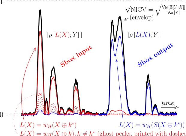
Therefore, the NICV is the envelop or maximum of all possible correlations computable fromX withY. As a consequence of the Cauchy-Schwarz theorem, there is an equality in (4) if and only ifL(x) =E[Y_|X =x], which is the optimal prediction function2.

In practice, the (square) CPA value does not attain the NICV value, owing to noise and other imperfections. This is illustrated in Fig. 1. The difference can come from various reasons like:

• The attacker knows the exact prediction function, but as usual not the actual key. For instance, let us assume the traces can be written as Y =wH(S(X⊕k?)) +N, wherek? ∈F82 is the correct key,S:F82 →F82 is a substitution box, wH is the Hamming weight function, and N is

some measurement noise, that typically follows a centered normal dis-tribution N _{∼ N}(0, σ2_{). In this case, the optimal prediction function} L(x) = E[Y_|X =x] is equal to: L(x) = wH(S(X ⊕k?)) (the only

hy-pothesis on the noise is that it iscentered andmixed additively with the sensitive variable). This argument is at the base of the soundness of CPA:

∀k₆=k?, ρ[wH(S(X⊕k));Y]≤ρ[wH(S(X⊕k?));Y]

≤pVar[E[Y_|X]]/Var[Y].

• The CPA is smaller than NICV when the attacker assumes a wrong model, for instanceL(x) =wH(x⊕k?), whenY =wH(S(x⊕k?)) +N.

• Eventually, the attacker can have an approximation of the leakage model, for instanceL(x) =wH(S(x⊕k?)), whereas actuallyY =P8i=1βi·Si(x⊕

k?_{) +N, where β}

i ≈ 1, but slightly deviate from one (a.k.a. stochastic

model [32]).

The distance between CPA and NICV is, innon-information theoretic attacks (i.e., attacks in the proportional / ordinal scale, as opposed to the nominal scale [37]) similar to the distance between perceived information (PI) and mu-tual information (MI) [29]. Like CPA, NICV also achieves an asymptotically constant value, once the measurement set has reached a representative sample size.

It can also be noted that NICV is considered as the relevant distinguisher for the Linear Regression Analysis (LRA) [19,22], which acts as the CPA but with a parametric leakage model.

Now, ifX is uniformly distributed, the NICV in itselfis nota distinguisher.

L

(

X

) =

w

(

X

⊕

k

)

L

(

X

) =

w

(

X

⊕

k

)

, k

6

=

k

(ghost peaks, printed with dashed lines)

L

(

X

) =

w

(

S

(

X

⊕

k

))

Sb

ox

inp

ut

Sb

ox

ou

tp

ut

1

0

(envelop)

|

ρ

[

L

(

X

)

;

Y

]

|

|

ρ

[

L

(

X

)

;

Y

]

|

√

NICV =

q

time

Figure 1: Illustration on NICV metric whenY =P8_i=1βi·Si(x⊕k?) +N, and

Indeed, if we assume thatY =wH(S(X⊕k?)) +N, then:

Var[E[Y_|X]] =P_x∈XP[X =x]E[Y_|X =x]2₋E[Y]2 = ₂18

P

x∈XE[wH(S(x⊕k?)) +N]

2

− Px∈XE[wH(S(x⊕k?)) +N]

2

= ₂18

P

x0_=x⊕k?_∈XE[wH(S(x0))]

2

− Px0_=x⊕k?_∈XE[wH(S(x0))]

2

=Var[wH(S(X))] .

On the other hand,Var[Y] =Var[wH(S(X))] +Var[N]. All in one:

NICV = Var[E[Y|X]]

Var[Y] = 1 1

SNR+ 1

, (5)

where the signal-to-noise ratio SNR is the ratio between:

• the signal, i.e., the variance of the informative part, namelyVar[wH(S(X⊕k?))],

and

• the noise, considered as the varianceVar[N].

Clearly, Eqn. (5) does not depend on the secret key k? as both Y and X are public parameters known to the attacker. Moreover, this expression is free from the leakage model L(X), which means that NICV does not depend on the implementation. Thus, NICV searches for all linear dependencies of public parameterXwith available leakage tracesY independant of the implementation. In case of protected implementation, if the countermeasure removes all linear leakages related to X, then the NICV should also eventually suppress. On the other hand, NICV can detect accidental linear leakage from a protected implementation.

Remark 1 In the binary case (n= 2) when both classes are equally probable,

the expression of NICV simplifies to: NICV=Var[E[Y|X]] Var[Y] =

(E[Y|X=0]−E[Y|X=1]

2 )

2

Var[Y] .

It is similar to Cohen’sd metric.

Now comparing NICV with other leakage detection techniques like SOST and SOSD we can give the following remarks.

Remark 2 SOSD is actually proportional to the inter-class variance (this point

And thus:

X

i,j

(Ti−Tj)2= 2×2n

X

i

T_i2₋2 X

i

Ti

!2 =

2_×22nX

x

EY2_|X =xP[x]₋2 28E[Y]2

= 22n+1Var[E[Y_|X]] .

But this inter-class variance is not normalized. Therefore, the SOSD can be large at samples whereVar[N] is large, although not containing (much) infor-mation.

Remark 3 SOST which was proposed as an improvement over SOSD is nor-malized. Using our notations, SOST is equal to

m X

(x,x0_)∈X2

(E[Y_|X =x]₋E[Y_|X =x0])2 q

Var[E[Y|X=x]] P[X=x] +

Var[E[Y|X=x0_]] P[X=x0_]

,

where m is the number of traces. This certainly is an expression that is not usual in statistics, and a prioricannot be simplified. At the opposite, NICV can be meaningfully expressed as a function of the CPA attack (recall Eqn.(4)).

3.2

Estimation of NICV

The number of traces is m, and each trace is indexed by i. In the sequel, when we sum overi, we mean i = 1, . . . , m. Let (yi)i=1,...,m be side-channel

measurements, and (xi)i=1,...,m be plaintext bytes. We define the (empirical)

probability of a given plaintext byte:

ˆ

P(X =x) = 1 m

X

is.t. xi=x

1 .

and the (empirical) per-class average, for a given classx_{∈ {}0, . . . ,2n₋1_}:

ˆ

E(Y_|X =x) = X

is.t. xi=x

yi

!

/ X

is.t. xi=x

1 !

= 1

mPˆ(X=x) X

is.t. xi=x

yi ,

The numerator of the NICV is:

d

Var(ˆE(Y_|X)) = 1

2n

2_Xn−1

x=0 ˆ

P(X =x)Eˆ(Y_|X =x) 2

− ₂1n

2_Xn−1

x=0 ˆ

P(X=x)ˆE(Y_|X =x) !2

=

1 2n_m

2n₋₁ X

x=0 P

is.t.xi=xyi 2 P

is.t.xi=x1

− _m1 X

i

yi

Eventually, the (empirical) NICV is:

\

NICV = Var(ˆd E(Y|X)) d

Var(Y) = 1 2n_m

P2n₋₁

x=0

P

is.t.Xi=xyi 2

P

is.t.xi=x1 − 1

m

P

iyi

2

1

m

P

iy2i −

1

m

P

iyi

2 . (6)

We notice that Eqn. (6) can be estimated online using accumulators.

3.3

Lower Bound on the Number of Traces to Break the

Key (with CPA)

The success rate (0_≤SR_≤1) of an attack is the probability that is recovers the correct key. Regarding CPA, the success rate has been computed theoretically by Thillard, Prouff and Roche [36] (a result that extends the previous analytical formula obtained for the “difference-of-means” test by Fei, Luo and Ding [13]). It is related to the various factors of the experimental setup, namely:

• the signal-to-noise ratio (which is also directly related to the NICV metric – recall Eqn. (5)),

• the sensitive variable expression, which discriminates more or less easily the correct key (which relates to an algorithmic parameter known as the

confusion coefficient notedκ),

• the number of tracesm.

The expression takes the following form:

SR= Φ(√mΣ−1/2µ) .

In this expression, Φ is the cumulative distribution function of the multivariate Gaussian. LetNkbe the number of key hypotheses. ThenΣis a (Nk−1)×(Nk−

1) matrix, andµis column of length (Nk−1). In the worst case, the leakage

model is very discriminating. This means that the wrong key guesses are all equivalent and yield a null value for the distinguisher. It is a strong assumption, but for good ciphers, such as the AES, this pessimistic approximation is not too far from the reality [23]. In this case, Σ degenerates to a 1_×1 matrix (a scalar), equal to: Σ = 2σ2_(κ

0−κ1). This consists in the application of thedisintegration theorem, since the covariance matrix has not full rank. The problem is projected on a smaller matrix of size rank(Σ)_×rank(Σ) (in our case, 1_×1). In this equation,κ0 is a “generalized” confusion coefficient.

Also,µis a scalar, equal toκ0−κ1. So, we have:

SR= Φ r

m_×κ0−κ1 2σ2

!

. (7)

The ratio κ0−κ1

σ2 is the signal-to-noise ratio; owing to Eqn. (5), it is

equal to 11 NICV−1

So, for a given confidence level in the result of the attack, expressed as targetted success rate SR, we have that the lower bound on the number of traces to break the key ismSR, equal to:

m_SR= 2σ 2

κ0−κ1 ×

Φ−1(SR)2 , (8)

where Φ−1is the reciprocal function of Φ (recall that Φ is monotonic decreasing). The function Φ can be computed from the “error function” (in C code,erf)”: Φ(y) = 1₂ erf(y/√2) + 1. It can be checked that Φ−1(0.80)_≈0.84.

So, any CPA will require more traces to recover the key thanm_SR.

The equation (8) has a simple interpretation in a log-log graph, where the X axis isσand theY axis ism_SR. It simply cuts the plan into two halves, that are separated by a straight line (called “frontier”), of equation

log₂ mlower bound_SR

= 2 log₂

_σ

√_κ

0−κ1

+ 1 + 2 log₂ Φ−1(SR)

= 2 log₂

_σ

√_κ

0−κ1

+ 0.497 when SR= 80%. (9)

The possible attacks require a number of tracesm_SR, i.e., such asm_SR is above the “frontier”. A more precise characterization follows.

In [36], the confusion coefficient for the CPA is defined as:

κδ=

1 2n

X

x∈X

L(x_⊕k)_×L(x_⊕k?) Whereδ=k_⊕k?

= 1 2n

X

x∈X

L(x)_×L(x_⊕δ) = 1

2n(L⊗L)(δ) , (10)

where_⊗is the convolution function.

We consider the ideal case where L = wH(S(X⊕k))− n₂. This function

is defined to be balanced, i.e., P_x∈

Fn2L(x) = 0. In this case, for δ= 0: κ0 =

1 2n

P

x∈X wH(x)−n2 2

= n₄, which does not depend on the exactS.

The approximation that all incorrect keys yield a zero value for the distin-guisher amounts to say that_∀k₆= 0, κk =₂1n(L⊗L)(k) = 0.

So, κ0 =n/4 (= 2 for AES, where n= 8) andκ1 = 0, and thus Eqn. (11) becomes:

log₂ mlower bound_SR = 2 log₂(σ)₋0.503 whenSR= 80%. (11)

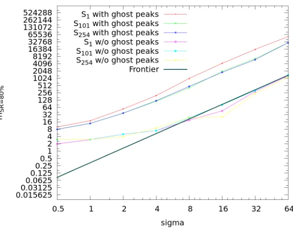
Figure 2: Simulatedm_SR=80%

in the graph are sometimes “anticipated” success rates (i.e., lower than what would have been obtained by smoothing the experimental success rate curves before selecting themsuch asSR(m) = 0.8).

We assume that the leakage is the Hamming weight of a sensitive variable, that has the formS(X _⊕k). The hypothesis _∀k ₆= 0, 1

2n(L⊗L)(k) = 0 is all

the more true asSis cryptographically strong. So we investigate different types of bijective sboxes: S(x) = axd

⊕b, where a and b are the constants also used in the AES. The operations_⊕andare respectively the addition and the multiplication in the Galois fieldF28. We consider three values ford:

1. d= 1, i.e., an affine function (the least non-linear),

2. d= 101, i.e., a medium function, and

3. d= 254, i.e., a good function (it is the AES SubBytes).

Those three substitution boxes are respectively noted S1, S101 and S254. In addition, for each sbox, we compute anidealleakage modelLno ghost peak_(X

⊕k), such that:

Lno ghost peak(X_⊕k) = (

wH(S(X⊕k?))−n₂ ifk=k?, or

wH(S(D))−n₂ otherwise,

To summarize, in Fig. 2, we compute for the three different sboxes S the two kinds of CPA:

• Withghost peaks:

ρ(wH(S(X⊕k?)) +N;wH(S(X⊕k)));

• Withoutghost peaks:

ρ wH(S(X⊕k?)) +N;Lno ghost peak(X⊕k)

.

Clearly, the attacks do not depend on the sbox in this later case, because we simply remove the rivals, which brings us to the case of distinguishing from two keys. Quite logically, this attack reaches the theoretical minimum. And we see that the less discriminating the sbox, the more traces are required.

Remark 4 The valuesκ(0)₋κ(1) in Eqn.(7)are computed using the leakage model of Eqn. (10) as: κ(0)₋maxδ6=0κ(δ) for the three studied substitution

boxes. Whenn= 8(like in the case of AES), it can be proven that whatever the bijective substitution box, κ(0) = n/4 = 2. The value of maxδ6=0κ(δ) depends

on the substitution box. Namely, we have:

    

ForS=S1: κ(0)−maxδ6=0κ(δ) = 0.5 ,

ForS=S101: κ(0)−maxδ6=0κ(δ) = 1.5 ,

ForS=S254: κ(0)−maxδ6=0κ(δ) = 1.625 .

Thus, for a given success rate (say80%) and a given noise variance σ2_{, if the}

number of traces to break without substitution box (that is,S=S1) ism1, then:

• the number of traces to recover the key withL(x_⊕k) =wH(S101(x⊕k))

would be m1×01..55 = 1

3m1≈0.333m1, and

• the number of traces to recover the key withL(x_⊕k) =wH(S254(x⊕k))

would be m1×₁0_.625.5 = ₁₃4m1≈0.308m1.

This means that the choice of the substitution boxes impacts the number of traces to extract the key in a factor of about1 to3.

3.4

Discussion

4

Use Cases

We detailed the theoretical soundness and advantages of NICV as a leakage detection technique in Sec.3. In this section, we apply NICV in practical side-channel evaluation scenarios. Several use cases of NICV are discussed in the following.

4.1

Accelerating Side-Channel Attacks

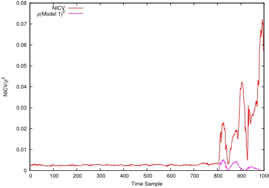
The main application of NICV is to find the interesting time samples for accel-erating SCA. A simple trace of an AES execution can have millions of points. Therefore it is of interest for the evaluator to know few interesting points rather than attacking the whole trace. We first apply the metric on traces of an AES-128 implementation running on an FPGA which performs one round per clock cycle. These traces are small and contain only 1,000 points. The comparison of our metric with a correlation coefficient computed with the good key is shown in Fig.3. The correlation is based on Hamming distance model of the state register of the AES core. The model can be expressed as wH(vali⊕valf) where vali

andvalf are initial and final value of the register. This leakage model is shown

to be very efficient in CMOS technology. A relevant peak of NICV is seen at the same moment as in correlation peak. Thus NICV is able to detect the point of leakage in the trace. It can be noticed that NICV curve shows several other peaks apart from the correlation peak. As shown later in Sec.4.2, other peaks in the NICV curve comes either from other leakage models or post-processing of cipher in the circuit.

0 0.01 0.02 0.03 0.04 0.05 0.06 0.07 0.08

0 100 200 300 400 500 600 700 800 900 1000

NICV/

ρ

2

Time Sample NICV

ρ(Model 1)2

Figure 3: NICV vs Correlation for a AES-128 hardware implementation

AddRoundKey SubBytes MixColumns

Column 1 Column 2 Column 3 Column 4 Row 2

Row 3 Row 4

ShiftRows

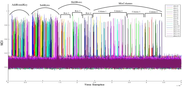
Figure 4: NICV computed for a AES-128 software implementation to detect each round operation

on an ATMEL AVR microcontroller. It is here that we can see the advantage of NICV. A single trace of this implementation contains 7 million points and needs roughly 5.3 Mbytes of disk space when stored in the most compressed format. These details are in respect to a LeCroy WaveRunner 6100A oscilloscope with a bandwidth of 1 GHz. We applied NICV on these traces to find the leakage points related to each of the 16 bytes of the AES. Fig.4shows the computation of NICV on the first round only (for better resolution of results). The computations of Sbox #0 for round 1 takes only_≈ 1,000 time samples. Once the interesting time samples corresponding to each executed operation is known, the trace size is compressed from 7,000,000 to 1,000, i.e., a gain of roughly 7,000_×in attack time.

One very interesting application of NICV that we found during our exper-iments is to reverse engineering. We computed NICV for all the 16 bytes of the plaintext and plotted the 16 NICV curves in Fig. 4 (depicted in different colors). By closely observing Fig. 4, we can distinguish individual operations from the sequence of byte execution. Each NICV curve (each color) shows all sensitive leakages related to that particular byte. Moreover, with a little knowl-edge of the algorithm, one can easily follow the execution of the algorithm. For example, the execution of all the bytes in a particular sequence indicates the SubBytes or AddRoundKey operation. Manipulation of bytes in sequence

4.2

Testing Leakage Models

A common problem in SCA is the choice of leakage model which directly affects the efficiency of the attack. As shown in Sec.3.1, the square of the correlation between modeled leakage (L(X, K)) and traces (Y =L(X, K?_{) +N) is smaller}

or equal to NICV, whereN represents a noise. The equality exists only if the modeled leakage is the same as the traces. We tested two different leakage models for the state register resent before the Sbox operation of AES, i.e., wH(vali⊕valf)∈J0,8K(Model 1) andvali⊕valf ∈J0,255K(Model 2). Similar models are built for another register intentionally introduced at the output of the Sbox, i.e.,wH(S(vali)⊕S(valf))∈J0,8K(Model 3) andS(vali)⊕S(valf)∈

J0,255K(Model 4). We implemented the AES on an FPGA and acquired SCA traces to compare the leakage models. Fig. 5 shows the square of correlation of four different leakage models with the traces against the NICV curve. It can be simply inferred from Fig. 5(b) that Model 4 performs the best while Model 2 is the worst. The gap between NICV andρ(Model 4)2 _{is quite large,} most probably due to reasons mentioned in Sec. 3.1. This means that there exist other leakage models which could perform better than Model 4. However, finding these models might not be easy because of limited knowledge of design and device characteristics available. Methods based on linear regression [11] can be leveraged to determine the most relevant leakage model.

4.3

Comparing Quality of Measurements

SNR is often used to estimate the quality of a measurement setup/traces to compare different measurement setups. The problem with SNR is that it is computed using a specific leakage model. NICV is a good candidate for quality comparison owing to the independence from choice of leakage model.

4.4

Ghost Peaks

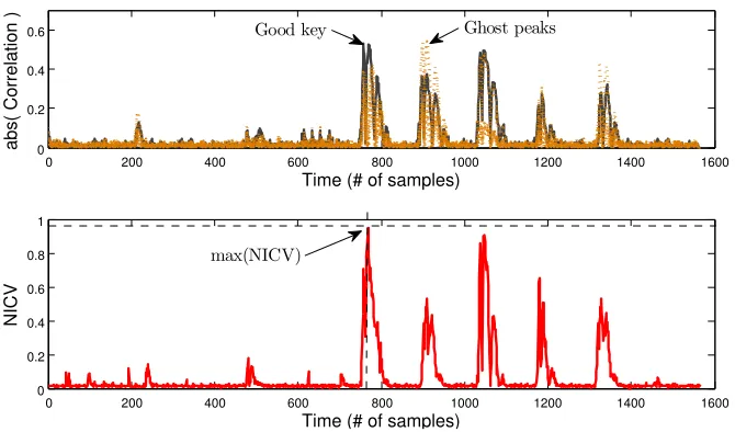
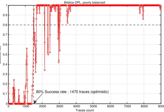
To further demonstrate the advantageous use of NICV, we implemented a bit-slice implementation (i.e., a single bit of plaintext is processed per cycle) of PRESENT algorithm on an ATMEL AVR microcontroller. Firstly we used NICV to localize the activity of an sbox in a multi-million sample trace. Figure6 (top) shows the result of a CPA on the least significant bit with 10,000 traces with an SNR of 15.8. Next we plot the NICV computed with respect to the input plaintext byte in Fig.6 (bottom). If we compute the success rate of an attack on the whole trace, the ghost peak around sample 900 leads to failure of the attack. However if we compute a success rate on a window around samples where NICV is maximal, we are able to suppress the ghost peak. The success rate of an attack around sample 800, where NICV is maximal is shown in Fig.7.

4.5

Accelerating SCA on Asymmetric Key Cryptography

0 0.01 0.02 0.03 0.04 0.05 0.06 0.07 0.08

0 100 200 300 400 500 600 700 800 900 1000

NICV/

ρ

2

Time Sample NICV

ρ(Model 1)2 ρ(Model 2)2 ρ(Model 3)2 ρ(Model 4)2

(a)

0 0.001 0.002 0.003 0.004 0.005 0.006

0 100 200 300 400 500 600 700 800 900 1000

ρ

2

Time Sample

ρ(Model 1)2

ρ(Model 2)2

ρ(Model 3)2

ρ(Model 4)2

(b)

Figure 5: (a) NICV vsρ2 _{of four different models, (b) and its zoom}

ex-0 200 400 600 800 1000 1200 1400 1600 0

0.2 0.4 0.6

Time (# of samples)

abs( Correlation )

0 200 400 600 800 1000 1200 1400 1600 0

0.2 0.4 0.6 0.8 1

Time (# of samples)

NICV

Ghost peaks Good key

max(NICV)

Figure 6: NICV vs Correlation depicting ghost peaks for a software implemen-tation of PRESENT protected by DPL (Dual-rail Precharged Logic)

ponentiation is illustrated in Alg.1, whereN is the modulus (e.g., that fits on 1024 bits), andR[1] andR[2] are two 1024 bit temporary registers. Let us call di the 1024 bits ofd. We assumed0= 1.

Hence the numberX3 _{will be computed (inR[1]; refer to line5) if and only} ifd1= 1. This conditional operation is at the basis of the SCA on RSA [25]: if a correlation between the tracesY and the prediction L(X) =X3 _{exists, then} d1 = 1; otherwise, d1 = 0. For this alternative to be tested with NICV, one should compute Y_|X3, where X3 (modulo N) is a large number (e.g., 1,024 bits). To be tractable, small parts of X3 like the least significant byte (LSB) shall be used instead of X3. In this case, a leakage can be detected by com-putingVarEY_|LSB(X3_{)/Var[Y]. The corresponding attack would use the} prediction functionL(X) = LSB(X3_).

For sure, the test is relevant only if the bit d1 is set in the private key d. But if it is not, then maybed2 is set. In this case, a leakage can be detected by computing

VarEY_|LSB(X5_{)/Var[Y]. Similarly, if d}

1 = d2 = 0, it is plausible that d3 = 1, and thus X9 is computed. Thus, it is sufficient, in order to detect a leakage to compute

0 1000 2000 3000 4000 5000 6000 7000 8000 9000 0

0.1 0.2 0.3 0.4 0.5 0.6 0.7 0.8 0.9

1 Bitslice DPL, poorly balanced

Traces count

Success rate

80% Success rate : 1470 traces (optimistic)

Figure 7: Success rate of CPA on a software implementation of PRESENT protected by DPL after suppression of ghost peaks using NICV

If, for example, the 10 NICV quantities VarhEhY_|LSB(X2i+1)ii/Var[Y], for 1_≤i_≤10, are computed (without knowing the keyd), then a vulnerability is detected with probability 1₋2−10 _{(indeed, 2}−10 _{is the probability of having} d1=. . .=d10= 0). This methodology is illustrated in Fig.8.

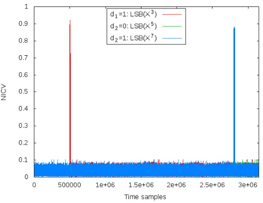
The methodology has been validated in practice, on RSA with an exponent d= (. . .111)2, i.e., finishing with three bits at 1. In Fig.9, we have computed NICV by partitioning on LSB(X3)_{∈ {}0, . . . ,255_}. The NICV indeed features a peak, which validates thatd1 = 1, and that the device leaks. As the peak is really sharp, the leak is strong (our implementation is an ATMega163 smartcard, which is known to leak a lot). For cross-checking, we also plotted in Fig.9:

• NICV on LSB(X5_{), which does not feature a peak (as expected). It would} have had a peak if the exponent would have beend= (. . .101)2.

• NICV on LSB(X7_{), which has a peak, as expected.}

5

Conclusions and Perspectives

Algorithm 1:Unprotected right-to-left 1024 bit RSA implementation

Input :X _∈ZN, d= (d1023,· · · , d0)2

Output:Xd

∈ZN

1 R[1]←1

2 R[2]←X

3 fori∈_J0,1023_Kdo 4 if di= 1then

5 R[1]←R[2]·R[1] /* Multiply */

6 end

7 R[2]←R[2]·R[2] /* Square */

8 end

9 returnR[1]

Var[E[Y|LSB(X5_)]] Var[Y]

Var[E[Y|LSB(X9_)]] Var[Y] Var[E[Y|LSB(X3_)]]

Var[Y]

There is peak There isnopeak

Caption: ...

Leak detected

d1= 1

d2= 1

d3= 1

No leak... ...with proba

≥1−2−10

R[1] =X3

R[1] =X5

R[1] =X9

X X2 _X4 _X8 _X16 _...

R[2] :

Figure 9: Result of the methodology of NICV applied to RSA (first two steps of Fig.8)

as a distinguisher for an attack. Unlike templates, NICV can operate on the same set of traces which are used for attack. We can also use NICV to theoreti-cally estimate the lower bound on number of traces to attack an implementation with CPA. We demonstrated the power of NICV in several use cases related to SCA like detecting relevant time samples, comparing leakage models, detecting ghost peaks, etc.

Future works can focus on extending the power of NICV in detecting higher-order leakage and extensive application to asymmetric key cryptography.

Acknowledgements

References

[1] M. A. E. Aabid, S. Guilley, and P. Hoogvorst. Template Attacks with a Power Model. Cryptology ePrint Archive, Report 2007/443, December 2007. http://eprint.iacr.org/2007/443/.

[2] C. Archambeau, ´E. Peeters, F.-X. Standaert, and J.-J. Quisquater. Tem-plate Attacks in Principal Subspaces. In CHES, volume 4249 of LNCS, pages 1–14. Springer, October 10-13 2006. Yokohama, Japan.

[3] L. Batina, B. Gierlichs, and K. Lemke-Rust. Differential Cluster Analysis. In C. Clavier and K. Gaj, editors, Cryptographic Hardware and Embedded Systems – CHES 2009, volume 5747 ofLecture Notes in Computer Science, pages 112–127, Lausanne, Switzerland, 2009. Springer-Verlag.

[4] ´E. Brier, C. Clavier, and F. Olivier. Correlation Power Analysis with a Leakage Model. In CHES, volume 3156 of LNCS, pages 16–29. Springer, August 11–13 2004. Cambridge, MA, USA.

[5] S. Chari, J. R. Rao, and P. Rohatgi. Template Attacks. InCHES, volume 2523 of LNCS, pages 13–28. Springer, August 2002. San Francisco Bay (Redwood City), USA.

[6] O. Choudary and M. G. Kuhn. Efficient Template Attacks. Cryptology ePrint Archive, Report 2013/770, 2013. http://eprint.iacr.org/2013/ 770.

[7] C. C. Consortium. Common Criteria (akaCC) for Information Technology Security Evaluation (ISO/IEC 15408), 2013.

Website: http://www.commoncriteriaportal.org/.

[8] J. Cooper, G. Goodwill, J. Jaffe, G. Kenworthy, and P. Rohatgi. Test Vector Leakage Assessment (TVLA) Methodology in Practice, Sept 24–26 2013. International Cryptographic Module Conference (ICMC), Holiday Inn Gaithersburg, MD, USA.

[9] J.-S. Coron, P. C. Kocher, and D. Naccache. Statistics and Secret Leak-age. InFinancial Cryptography, volume 1962 ofLecture Notes in Computer Science, pages 157–173. Springer, February 20-24 2000. Anguilla, British West Indies.

[10] J.-L. Danger, N. Debande, S. Guilley, and Y. Souissi. High-order Timing Attacks. In Proceedings of the First Workshop on Cryptography and Se-curity in Computing Systems, CS2 ’14, pages 7–12, New York, NY, USA, 2014. ACM.

[12] R. J. Easter, J.-P. Quemard, and J. Kondo. Text for ISO/IEC 1st CD 17825 – Information technology – Security techniques – Non-invasive attack mit-igation test metrics for cryptographic modules, March 22 2014. Prepared within ISO/IEC JTC 1/SC 27/WG 3. (Online).

[13] Y. Fei, Q. Luo, and A. A. Ding. A Statistical Model for DPA with Novel Algorithmic Confusion Analysis. In E. Prouff and P. Schaumont, editors,

CHES, volume 7428 ofLNCS, pages 233–250. Springer, 2012.

[14] B. Gierlichs, K. Lemke-Rust, and C. Paar. Templates vs. Stochastic Meth-ods. InCHES, volume 4249 ofLNCS, pages 15–29. Springer, October 10-13 2006. Yokohama, Japan.

[15] G. Goodwill, B. Jun, J. Jaffe, and P. Rohatgi. A testing methodology for side-channel resistance validation, September 2011. NIST Non-Invasive Attack Testing Workshop, http://csrc.nist.gov/news_events/

non-invasive-attack-testing-workshop/papers/08_Goodwill.pdf.

[16] S. Guilley, S. Chaudhuri, L. Sauvage, P. Hoogvorst, R. Pacalet, and G. M. Bertoni. Security Evaluation of WDDL and SecLib Countermeasures against Power Attacks. IEEE Transactions on Computers, 57(11):1482– 1497, nov 2008.

[17] S. Guilley, R. Nguyen, and L. Sauvage. Non-Invasive Attacks Testing: Feed-back on Relevant Methods, Sept 24–26 2013. International Cryptographic Module Conference (ICMC), Holiday Inn Gaithersburg, MD, USA.

[18] S. Hajra and D. Mukhopadhyay. SNR to Success Rate: Reaching the Limit of Non-Profiling DPA. Cryptology ePrint Archive, Report 2013/865, 2013.

http://eprint.iacr.org/2013/865/.

[19] A. Heuser, W. Schindler, and M. St¨ottinger. Revealing side-channel issues of complex circuits by enhanced leakage models. In W. Rosenstiel and L. Thiele, editors,DATE, pages 1179–1184. IEEE, 2012.

[20] I. T. Jolliffe. Principal Component Analysis. Springer Series in Statistics, 2002. ISBN: 0387954422.

[21] P. Karsmakers, B. Gierlichs, K. Pelckmans, K. D. Cock, J. Suykens, B. Pre-neel, and B. D. Moor. Side channel attacks on cryptographic devices as a classification problem. COSIC technical report, 2009.

[22] V. Lomn´e, E. Prouff, and T. Roche. Behind the scene of side channel attacks. In K. Sako and P. Sarkar, editors,ASIACRYPT (1), volume 8269 ofLNCS, pages 506–525. Springer, 2013.

[24] S. Mangard, E. Oswald, and F.-X. Standaert. One for All - All for One: Unifying Standard DPA Attacks.Information Security, IET, 5(2):100–111, 2011. ISSN: 1751-8709 ; Digital Object Identifier: 10.1049/iet-ifs.2010.0096.

[25] T. S. Messerges, E. A. Dabbish, and R. H. Sloan. Power Analysis Attacks of Modular Exponentiation in Smartcards. In C¸ . K. Ko¸c and C. Paar, editors,

CHES, volume 1717 ofLNCS, pages 144–157. Springer, 1999.

[26] A. Moradi, S. Guilley, and A. Heuser. Detecting Hidden Leakages. In I. Boureanu, P. Owesarski, and S. Vaudenay, editors,ACNS, volume 8479. Springer, June 10-13 2014. 12th International Conference on Applied Cryp-tography and Network Security, Lausanne, Switzerland.

[27] A. Moradi, O. Mischke, and T. Eisenbarth. Correlation-Enhanced Power Analysis Collision Attack. InCHES, volume 6225 ofLecture Notes in Com-puter Science, pages 125–139. Springer, August 17-20 2010. Santa Barbara, CA, USA.

[28] E. Prouff, M. Rivain, and R. Bevan. Statistical Analysis of Second Order Differential Power Analysis. IEEE Trans. Computers, 58(6):799–811, 2009.

[29] M. Renauld, F.-X. Standaert, N. Veyrat-Charvillon, D. Kamel, and D. Flandre. A Formal Study of Power Variability Issues and Side-Channel Attacks for Nanoscale Devices. In EUROCRYPT, volume 6632 ofLNCS, pages 109–128. Springer, May 2011. Tallinn, Estonia.

[30] R. L. Rivest, A. Shamir, and L. M. Adleman. A Method for Obtaining Digital Signatures and Public-Key Cryptosystems. Communications of the ACM, 21(2):120–126, 1978.

[31] A. Roche, G. Malandain, X. Pennec, and N. Ayache. The Correlation Ra-tio as a New Similarity Measure for Multimodal Image RegistraRa-tion. In W. M. W. III, A. C. F. Colchester, and S. L. Delp, editors,Medical Image Computing and Computer-Assisted Intervention - MICCAI’98, First Inter-national Conference, Cambridge, MA, USA, October 11-13, 1998, Proceed-ings, volume 1496 ofLecture Notes in Computer Science, pages 1115–1124. Springer, 1998.

[32] W. Schindler, K. Lemke, and C. Paar. A Stochastic Model for Differen-tial Side Channel Cryptanalysis. In LNCS, editor,CHES, volume 3659 of

LNCS, pages 30–46. Springer, Sept 2005. Edinburgh, Scotland, UK.

[34] Y. Souissi, M. Nassar, S. Guilley, J.-L. Danger, and F. Flament. First Principal Components Analysis: A New Side Channel Distinguisher. In K. H. Rhee and D. Nyang, editors, ICISC, volume 6829 ofLecture Notes in Computer Science, pages 407–419. Springer, 2010.

[35] F.-X. Standaert, B. Gierlichs, and I. Verbauwhede. Partition vs. Compar-ison Side-Channel Distinguishers: An Empirical Evaluation of Statistical Tests for Univariate Side-Channel Attacks against Two Unprotected CMOS Devices. In ICISC, volume 5461 of LNCS, pages 253–267. Springer, De-cember 3-5 2008. Seoul, Korea.

[36] A. Thillard, E. Prouff, and T. Roche. Success through Confidence: Evalu-ating the Effectiveness of a Side-Channel Attack. In G. Bertoni and J.-S. Coron, editors,CHES, volume 8086 ofLecture Notes in Computer Science, pages 21–36. Springer, 2013.

[37] C. Whitnall, E. Oswald, and F.-X. Standaert. The Myth of Generic DPA . . . and the Magic of Learning. In J. Benaloh, editor, CT-RSA, volume 8366 ofLecture Notes in Computer Science, pages 183–205. Springer, 2014.

[38] D. W. Zimmerman, B. D. Zumbo, and R. H. Williams. Bias in Estimation and Hypothesis Testing of Correlation. Psicol´ogica, 24:133–158, 2003.

A

NICV

vs.

TVLA

NICV and TVLA are two methods to quantify the leakage of a cryptographic module (CM). They have been discussed recently at the first International Cryp-tographic Module Conference (09/2013), respectively in presentations [17] and [8].

TVLA consists in operating the CM with a fixed key (specified), exercised under afixed input message, and undervarying messages [15, Sec. 3]. Then, a T-test (See Eqn. (1), forn= 2 classes) is applied on both sets of measurements.

A.1

Differences

TVLA requires the definition of a set of keys and messages to be tested. This has some side effects. First, it is not always possible to set a key or an input message in a CM; indeed, the key is often initialized randomly or agreed by a protocol, and in most modes of operation, the input message depends upon an initialization vector (IV) that cannot be chosen. Second, this is restrictive as a general method, because new or regional algorithms are created frequently, hence the key / message database of TVLA must keep track of this evolution. Third and the criteria for the selection of keys & inputs is delicate to explain, hence possibly suspicious. At the opposite, with NICV, the device can be tested with its operational key and without chosen inputs.

messages, whereas NICV tests whether the leakage varies of a multiplicity of

different inputs (hence the computation of avariance). Also, NICV can focus on each input bit (n= 1) or byte (n= 8).

A.2

Common Points

As underlined in Remark2, SOSD and the inter-class variance are proportional. Thus SOST (normalized version of SOSD) and NICV are related, for binary partitionings (i.e., when there are onlyn= 2 classes).

Also, both NICV and TVLA can have an estimation of their bias: the con-fidence level of NICV is discussed in [23,38], and in [8] for TVLA.