Three Essays on Realized Volatility Models for High-Frequency Data.

(1)

Abstract

SHEN, JI. Three Essays on Realized Volatility Models for High-Frequency Data. (Under the direction of Denis Pelletier.)

The dissertation centers on modeling volatility of stock returns with high frequency data. It contains three chapters.

In Chapter 1, we propose a multivariate realized GARCH model where the conditional variance of daily returns depends on lagged realized measures of volatility computed with high-frequency data. In turn, a measurement equation contemporaneously links the realized measures and the conditional variance. To greatly reduce the number of parameters in the measurement equation, we use adaptive Lasso and the least-angle regression algorithm. For the GARCH dynamic of the conditional variance, we favor a diagonal BEKK structure applied to rotated variables. Our empirical results suggest that the use of variable selection with adaptive Lasso for the measurement equation instead of OLS leads to improved out-of-sample forecasting performances.

In Chapter 2, we introduced a realized Markov regime-switching BEKK model which generalizes the BEKK model by using two regimes featuring different variance dynamic specifications. Within each regime, we use a BEKK model to govern the variance. The persistence of both regimes yields an extra source of volatility persistence compared with standard, single-regime BEKK, thereby enhancing the flexibility in describing the volatility persistence of shocks. To reduce the parameters in estimation, we implement covariance targeting with rotated variables. The empirical evidence shows that the regime-switching BEKK model has a significantly better performance in both in-sample fit and out-of-sample forecasting.

(2)

(3)

(4)

Three Essays on Realized Volatility Models for High-Frequency Data

by Ji Shen

A dissertation submitted to the Graduate Faculty of North Carolina State University

in partial fulfillment of the requirements for the Degree of

Doctor of Philosophy

Economics

Raleigh, North Carolina 2017

APPROVED BY:

Barry Goodwin Walter Thurman

Peter Bloomfield Minor Member

(5)

Dedication

(6)

Biography

(7)

Acknowledgements

I would like to thank my advisor Dr. Denis Pelletier for his direction and guidance to my research. Through patient discussion he has provided me the knowledge and motivation to overcome one hurdle after another.

I would also like to thank my committee members: Dr. Peter Bloomfield, Dr. Barry Goodwin and Dr. Walter Thurman. Their valuable comments and suggestions greatly enriched this dissertation. I am also deeply grateful for their support and encouragement.

(8)

List of Tables

Table 1.1 Parameter Estimates of the matrixA˜in the rotated RBEKK model . . . 26

Table 1.2 Parameter Estimates of the matrixB˜ in the rotated RBEKK model . . . 26

Table 1.3 Fit for Measurement Equation Estimators (1.8) . . . 28

Table 1.4 Estimates of coefficient matrixΓ . . . 32

Table 1.5 Statistical Test of Predictive Ability . . . 36

Table 1.6 Gain of predictive covariance using ALasso . . . 38

Table 2.1 Summary Statistics of Daily Return . . . 58

Table 2.2 Summary Statistics of Realized Volatility . . . 58

Table 2.3 Estimation of coefficient . . . 60

Table 2.4 Markov Transition Probability . . . 60

Table 2.5 Statistical Test of Predictive Ability . . . 73

Table 3.1 Markov Transition Probability . . . 77

Table 3.2 Estimation of GARCH Coefficient . . . 87

Table 3.3 Estimation of coefficient measurement equation . . . 88

(11)

List of Figures

Figure 1.1 ALasso shrinkage of the coefficients of the first measurement equation in (1.8). 29 Figure 1.2 Shrinkage of Degrees of Freedom. DF refers to the number of non-zero parameters. 29

Figure 1.3 Mean Squared Error ALasso as a function of relative model size . . . 30

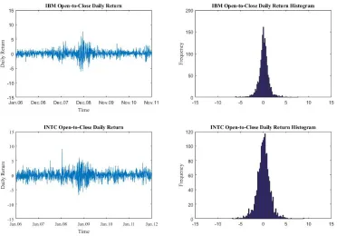
Figure 2.1 The open-to-close log daily return of IBM and INTC. . . 54

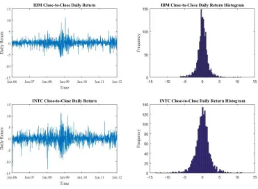
Figure 2.2 The close-to-close log daily return of IBM and INTC. . . 55

Figure 2.3 The annualized realized volatility and co-volatility of IBM and INTC. . . 57

Figure 2.4 Probability of staying in responsive regime (regime 2) . . . 64

Figure 2.5 The impact of one standard deviation innovation of IBM. . . 68

Figure 3.1 The filtered probabilities of FTP (upper panel) and TVTP (lower panel) in the responsive regime (regime 2). . . 85

Figure A.1 The open-to-close log daily return of AXP,BAC,DD,GE,IBM. . . 102

Figure A.2 The open-to-close log daily return of INTC,JPM,KO,MSFT,XOM. . . 103

Figure A.3 The annualized realized volatility of AXP,BAC,DD,GE,IBM. . . 104

(12)

Chapter 1

Realized Rotated BEKK Model

1.1 Introduction

(13)

the MEM to squared returns and realized volatility as separate models. The univariate and multivariate HEAVY models introduced by Shephard and Sheppard (2010) and Noureldin, Shephard, and Sheppard (2012) consider a system including a measurement equation for multi-step forecasting of the conditional variance of daily returns. The mathematical structure of the HEAVY model is a generalization of the MEM framework.

While the HEAVY model postulates GARCH-type dynamics for the realized measure by modelling its conditional expectation, the univariate realized GARCH model introduced by Hansen, Huang, and Shek (2012) relate the realized measure itself to conditional variance and a term that captures leverage effects. The basic idea is that the connection between the realized measure and the conditional variance can be used to update the realized measure process, thus providing a recursive prediction of the con-ditional variance of the asset. Almost universally, the incorporation of realized measures into volatility models has led to large economic and statistical gains (Christoffersen, Jacobs, and Mimouni, 2010; Do-brev and Szerszen, 2010). Forecast gains tend to be more pronounced at short time horizons, typically the first several days. All of the models mentioned above focus on a small number of assets. For exam-ple, multivariate HEAVY models separate ten assets into five groups, and deal with two assets in each group. In general, most of these models suffer from a curse-of-dimensionality problem that constrains their practical application.

Automatic model-building methods are familiar in the linear model literature. They are used to automatically produce better models in terms of prediction accuracy and parsimony. One promising model-building method is the Lasso; its computationally simpler variation called Least Angle Regres-sion (LARS) will be applied here.

(14)

1.2 Literature Review

1.2.1 Univariate Volatility Models

In financial econometrics, the autoregressive conditional heteroskedasticity (ARCH) model is a bench-mark tool for analyzing the time-variation of conditional variance. The ARCH model is essentially an ARMA model for the squared return and many tools of standard, linear time-series analysis can be di-rectly applied. The family of ARCH models is easy to estimate; these parsimonious models are capable of providing good descriptions of the dynamics of asset volatility. The complete ARCH(p) model relates the current level of volatility to pastpsquare shocks (Engle, 1982). Considerrt, which denotes the log

return of a single asset, and is characterized as a real-valued discrete-time stochastic process. We model rtas

rt=µt+t

whereµtcan be any general model for the conditional mean (e.g. autoregressive (AR) model, moving

average (MA) model, autoregressive integrated moving average (ARIMA) model, etc). In practice, the model for the conditional mean should be flexible enough to capture the dynamics present in the data. For many financial time series, particularly those measured over short intervals such as one day or one week, assumingµt= 0is appropriate. As for the error term,

var(rt|Ft−1) =E(2t|Ft−1) =ht,

t=h1t/2et,

whereh1_t/2 is a positive real value andFt−1is the set of all information up to timet−1. Also, assume the random variableetmeets two moment conditions:

E(et|Ft−1) = 0,

(15)

For an ARCH(1), the variance process is given by

ht=ω+α2t−1.

They key feature of this model is that the conditional variance of the shock, t, is time varying and

depends on past values through its square. The varianceht is the timet−1 conditional variance and

is measurable in Ft−1. The generalized ARCH (GARCH) process, introduced by Bollerslev (1986),

improves the original specification by adding lagged conditional variances. These lagged terms essen-tially act as “smoothing” terms. GARCH models typically fit as well as higher ordered ARCH models while remaining relatively parsimonious. The conditional variance in a GARCH(1,1) process evolves according to

ht=ω+α2t−1+βht−1.

In this specification, the conditional variance is an average of the lagged shock,2_t₋₁, and the lagged variance,ht−1, plus a constant. The effect of the lagged variance is to produce a model that is actually

an ARCH(∞). This result is readily obtained by continued backward substitution of the conditional variance. To ensure the conditional variances are always positive, restrictions must be imposed on the parameters of the GARCH model. In a GARCH(1,1), these restrictions areω > 0, α≥0, andβ ≥ 0. The unconditional variance can be derived as

¯

h≡E[ht] = ω

1−α−β.

The GARCH model with1−α−β >0is covariance stationary as long as the model for the conditional mean corresponds to a stationary process.

1.2.2 The BEKK Model

(16)

the BEKK is that quadratic forms are positive semi-definite, and the sum of a positive semi-definite matrix and a positive definite matrix is positive definite. The model specification is an extension of the univariate model. Specifically, consider a vector of returnsrtof dimensionk×1. Similar to the setup

in the univariate case,

rt=µt+t, (1.1)

whereµtis a general time series model for the conditional mean vector. The conditional variance is

cov(t|Ft−1) =Ht

whereHtis ak×kpositive definite matrix and

t=Ht1/2et

whereH_t1/2can be obtained by the Cholesky factorization ofHt. The moment conditions

E(et|Ft−1) = 0

cov(et|Ft−1) =Ik

must also hold, with Ik denoting thek dimensional identity matrix. The covariance in a BEKK(1,1)

model evolves according to

Ht=CC0+B Ht−1B0+A t−10t−1A0

whereCis ak×klower triangular matrix and A and B arek×kparameter matrices. The elements of Htdepend on both squared returns and the cross-product of returns.

1.2.3 Realized Volatility

(17)

corre-sponding measure is the realized variance. Consider a log-price process,pt, driven by a standard Wiener

process with time-varying drift and stochastic volatility,

dpt=µtdt+σtdWt. (1.2)

where µt is of finite variation and σt is strictly positive and square integrable. Realized variance is

constructed by frequently sampling pt throughout the trading day. Suppose that prices on daytwere

sampled on a regular grid ofn+ 1points (0,1, ..., n) and letpi,t denote theithobservation of the log

price on dayt. Then-sample realized variance is defined as

RV_tn= n

X

i=1

(pi,t−pi−1,t)2 = n

X

i=1

r2_i,t. (1.3)

RV_tn is a consistent estimator of the integrated variance under the assumption of no market micro-structure noise, which includes bid-ask bounce, discreteness of price changes, etc:

lim n→∞RV

n

t =

Z t+1

t

σ_s2ds,

where the bounds tand t+ 1 represent the (arbitrary) interval over which the realized covariance is computed andnis typically somewhere between 13 (30-minute returns) and 390 (1-minute returns).

(18)

Shephard (2008) propose a realized kernel estimator which is consistent under the general conditions, e.g., higher-order dependence or endogeneity in the noise process, and robust to jumps. The idea is to capture (potentially noise induced) serial correlations in trade-to-trade returns by a kernel. The realized kernel estimator (RK) is defined as:

RK =γ0+

Q

X

q=1 k

q−1

Q

(γq+γ−q), (1.4)

with

γq = n

X

i=q+1

riri−q, f or q≥0,

wherek(·)is a kernel weighting function andk(0) = 1, k(1) = 0;Qis a bandwidth parameter which is chosen to minimize mean square error (MSE).

The multivariate case retains many of the features of the univariate case. For a multivariate process, the measure of interest is the realized variance/covariance matrix. Assume that thek×1log-price vector, P(t), is governed by the following multivariate diffusion process

dPt=Utdt+ ΩtdWt

whereUtis thek×1drift vector andΣt = ΩtΩ0t is instantaneous covariance.dWt denotes k-variate

mutually independent Brownian motion. Realized covariance estimates the integrated covariance matrix

Z t+1

t

Σsds.

Realized covariance is computed using the outer-product of the high-frequency returns,

RCt= n

X

i=1

ri,tri,t0 = n

X

i=1

(pi,t−pi−1,t)(pi,t−pi−1,t)0

(19)

covariance estimator. However, frequent sampling leads to practical difficulties since transaction prices are contaminated by noise (e.g. bid-ask bounce) and not perfectly synchronized (Epps, 1979).

Barndorff-Nielsen, Hansen, Lunde, and Shephard (2011) proposed the multivariate realized kernel which uses a “refresh time” sampling procedure to adapt the sampling scheme to the trading intensity of the least active asset at any given time within a day. The kernel also includes a well-chosen weight function for the lead and lag returns used in the computation of the covariance matrix. This ensures con-sistency of the estimator, while also guaranteeing positive semi-definiteness of the estimated covariance matrix. Formally, the multivariate realized kernel (RK) is defined as

RK = Γ0+

Q

X

q=1 K

q−1

Q

(Γq+ Γ0q) (1.5)

with

Γq =

˜

n

X

i=q+1

˜

ri˜r0i−q, forq≥0,

where r˜are refresh time returns, ˜nis the number of refresh time prices, K(·) is a kernel weighting function, and Q is a bandwidth parameter which is chosen to minimize mean square error (MSE). Refresh time returns are computed by sampling all prices and using last-price interpolation only when all assets have been traded. The recommended kernel is the non-flat Parzens kernel:

K(x) =

              

1−6x2+ 6x3 0> x≥1/2,

2(1−x)3 1/2> x≥1,

0 x >1.

(20)

will minimize the MSE caused by end-effects and the increased asymptotic variance due to reduction of the effective sample size. Settingm= 2is a common rule of thumb.

1.3 Realized BEKK Model

1.3.1 Definitions and Notation

In this section we introduce a new model, the realized BEKK (RBEKK) model. Similarly to the BEKK model in section 2.2, we start by assumingE(rt|Ft−1) = 0. This is a legitimate assumption based on several empirical studies. Otherwise, this condition could be met by reinterpretingrtas the return minus

its conditional mean. As a result,

rt=Ht1/2et, (1.6)

et i.i.d

∼ (0, Ik),

where Ik is the k×k identity matrix. The key quantity of interest in many financial applications is

the conditional variance/covariance,Ht =cov(rt|Ft−1). For the conditioned variance/covariance, we assume it follows the following dynamic:

Ht=CC0+B Ht−1B0+A Xt−1A0. (1.7)

In the standard GARCH(1, 1) modelHtis a function ofHt−1andrt−1r0t−1. In the present framework, a realized measure of variance/covariance Xt−1 will replacert−1rt0−1. In practice,Xt−1 could be the matrix of realized variance/covariance or a realized kernel. Thek×kmatrices A and B each havek2free parameters, while C is ak×klower triangular matrix withk∗ =k(k+ 1)/2free parameters. Under the assumption that the starting valueH0 is positive semidefinite, the parameterization in (1.7) guarantees thatHtis positive semidefinite for all t. Moreover, ifCis a full rank matrix, thenHtis positive definite

for all t. The coefficient matrix B determines the “smoothness” of the RBEKK model.

(21)

mea-surement equation in (1.8) to close the system:

xt=d+ Γht+ut (1.8)

uti.i.d∼ N(0,Σu)

wherext,d,ht, andutare allk∗ ×1 vectors,dis the intercept vector, andut is the innovation

vec-tor. Moreover,Γis a (k∗ ×k∗) constant coefficient matrix. This matrix characterizes the dependence between the realized measure and all of the elements of the conditional covariance matrix. A major feature of the RBEKK model is that the realized measure Xt can be linked with the

contemporane-ous logarithmicHtembedded in the measurement equation. Definext=vech(logmXt)and similarly ht = vech(logmHt)where the vech operator stacks the lower triangular portion, including the main

diagonal, of a (k×k) symmetric matrix into a (k∗ ×1)vector. Thelogmoperator gives the matrix logarithm which is a generalization of the element-wise logarithm (Higham, 2008). In our case, since the realized measure of variance/covariance is a real symmetric matrix, it can be decomposed into the product of a diagonal matrix of eigenvalues and a matrix of eigenvectors. Specifically, assumingXis the realized measure of variance/covariance, we can writeX = VXV˜ −1, whereV is the matrix of eigen-vectors ofX (each column of V is an eigenvector of X), and X˜ is a diagonal matrix whose diagonal elements are eigenvalues ofX. Replace each diagonal element ofX˜ by its natural logarithm to obtain

log ˜X. Then we havelogmX = V(log ˜X)V−1. Since the realized measure of variance/covariance is positive definite, the eigenvalues ofXare all positive. As a result,logmXis always a real, symmetric, and unique matrix.

The BEKK-type parameterization in (1.7) has O(k2) parameters. If the elements of A and B are unrestricted, which is a full parameterization, the evolution of every element inHt will be influenced

by its own lag as well as every cross-asset effect in the RBEKK model. A parsimonious specification is diagonal BEKK where the coefficient matrix A and B are assumed be diagonal. In this case, the equations for each element in the matrixHtcharacterize a group of univariate realized GARCH models

(22)

realized measure.

For demonstration, consider the 2 by 2 case of (1.7), with diagonal coefficient matrices.

     

h11,t

h12,t

h22,t

      =      

c2₁₁

c11c21

c2 21+c222

      +      

b2₁₁h11,t

b11b22h12,t

b2 22h22,t

      +      

a2₁₁x11,t

a11b22x12,t

a2 22x22,t

     

Although equation (1.8) has O(k4) parameters, the vectorized form is easy to estimate since its structure is amenable to seemingly unrelated regression (SUR). If a model has too many parameters, it begins to model the random noise in the data; this is commonly known as overfitting. Overfitting produces misleadingly high R-squared values and a reduced ability to make meaningful predictions. We use variable selection methods in estimation to reduce the number of elements in the coefficient matrix

Γ.

For demonstration, extend the previous example by writing out the 2 by 2 case of (1.8) in vech form:

     

x11,t

x21,t

x22,t

      =       d1 d2 d3       +      

γ11 γ12 γ13

γ21 γ22 γ23

γ21 γ22 γ33            

h11,t

h21,t

h22,t

      +      

u11,t

u21,t

u22,t

     

It is clear that each element in the realized covariance is a function of every component of the conditional covariance matrix. The RBEKK model fully specifies the dynamic system of daily returns and realized measure.

1.3.2 Covariance Targeting Under Rotation

(23)

tech-nique to keep the flexibility of dynamics in the full specification model while using the restricted model to reduce the parameters. The rotated GARCH models were introduced by Noureldin, Shephard, and Sheppard (2014). They compared scalar and diagonal rotated BEKK, DCC, and OGARCH models in the 10- and 30-dimensional cases. We apply this idea to the high-frequency volatility model. Assuming the process is stationary, the unconditional covariance of the daily return and expected realized measure are, respectively,V ar[rt] =E[Ht] = ¯HandE[Xt] = ¯X, the covariance targeting forHtis

Ht= ( ¯H−BHB¯ 0−AXA¯ 0) +B Ht−1B+A Xt−1A, (1.9)

assuming that( ¯H−BHB¯ 0−AXA¯ 0)is positive semidefinite. It is difficult to specify sufficient parameter restrictions to ensure that ( ¯H −BHB¯ 0−AXA¯ 0) is positive semidefinite. This feature of the model prevents the estimation of more flexible dynamics.

We fit the model with rotated variables to extend the idea of variance targeting to covariance tar-geting in multivariate models of any dimension. With the rotated variables we can estimate a restricted version of BEKK model which has fewer parameters to estimate while keep the flexibility of full speci-fied model. Define the rotated return as

et= ( ¯H1/2)−1rt= ¯H−1/2rt, (1.10)

we have

V ar(et) =Ik.

The conditional covariance of the rotated returns isV ar[et|Ft−1]≡H˜t, noting thatHt= ¯H1/2H˜tH¯1/2.

Similarly, for the realized measure of covariance, we haveXt= ¯X1/2X˜tX¯1/2, whereX˜tis the rotated

realized measure of covariance. This leads toH˜t = ¯H−1/2HtH¯−1/2 andX˜t = ¯X−1/2XtX¯−1/2. The

basic idea is that the variablesHtandXtare normalized by their unconditional expectations so that the

(24)

is

˜

Ht= (Ik−B˜B˜0−A˜A˜0) + ˜BH˜t−1B˜+ ˜AX˜t−1A˜ (1.11)

with

E[ ˜Ht] =E[ ˜Xt] =Ik.

This model has2k dynamic parameters since we assumeB˜ andA˜are diagonal. It is easy to impose positive definiteness on (Ik −B˜B˜0 −A˜A˜0) under this specification. For the conditional covariance

matrix of unrotated returnsHt, the BEKK model in (1.10) and (1.11) implies the original model in (1.7)

Ht= ¯H1/2H˜tH¯1/2=CC0+B Ht−1B0+A Xt−1A0 (1.12)

where

B = ¯H1/2B˜H¯−1/2, A= ¯H1/2A˜X¯−1/2, CC0= ¯H1/2(Ik−B˜B˜0−A˜A˜0) ¯H1/2 (1.13)

The rotated BEKK leads to a BEKK with full specification for the original variables, although the specification is constrained, sinceAandB depend on the Cholesky decomposition ofH¯ andX¯.

Bauwens, Laurent, and Rombouts (2006) discuss the invariance of multivariate models to linear transformations of returns. A transformed model is invariant if it keeps the same dynamic specification (in scalar, diagonal, and full parameterizations). They also note that BEKK models are invariant to linear transformations except in the case of diagonal dynamics. SinceA˜ is diagonal, directly derived from (1.13),Ais a full asymmetric matrix. This results in a fully parameterized BEKK model for the unrotated variables. In this sense, fitting a diagonal rotated RBEKK model allows for richer dynamics for the unrotated returns in practice because we avoid the curse-of-dimensionality.

(25)

i= 1, ..., k. This specification implies

˜

hij,t= (1−κij)1[i=j]+β 1/2

ii β

1/2

jj ˜hij,t−1+α

1/2

ii α

1/2

jj xij,t−1 (1.14) κij =α1_ii/2α1_jj/2+β_ii1/2β_jj1/2. (1.15)

for i, j = 1, ..., k. It is assumed thatα_ii1/2 > 0 andβ_ii1/2 > 0. The cross-equation parameter restric-tions between the variance and covariance equarestric-tions are a feature of BEKK-type parameterizarestric-tions. Covariance stationary is determined by the eigenvalues of the diagonal matrix A˜⊗A˜+ ˜B ⊗B˜. For the rotated model given in (1.10) and (1.11), we ensure covariance stationarity and also the positive definiteness of(Ik−B˜B˜0−A˜A˜0), where for anyk×kmatrixA˜with eigenvaluesκ1, . . . , κkand all k∈_Z+_{, ρ}₍_A_{) := max}

i|κi|.

Assumption 1 In the rotated RBEKK model given by (1.10) and (1.11), ρ( ˜A⊗A˜+ ˜B ⊗B˜) ≤ 1, α_ii1/2 >0, andβ_ii1/2 >0.

In practice,αii+βii<1is a necessary and sufficient condition for this assumption to hold and is easily

imposed in estimation (see Engle and Kroner, 1995).

1.3.3 Common Persistence Specification

In the rotated model,( ˜A⊗A˜+ ˜B⊗B˜)is a diagonal matrix with diagonal elementsκij =α1ii/2α

1/2

jj +

β_ii1/2β_jj1/2. We adopt the Noureldin, Shephard, and Sheppard’s (2014) common persistence (CP) speci-fication for the diagonal structures. The CP specispeci-fication imposes

κii=κ, i= 1, ..., k

implying common persistence for the diagonal elements ofH˜t. This results in the dynamic equation

˜

(26)

whereB˜is a diagonal matrix with elementsβ_ii1/2>0,A˜is a diagonal matrix with elements(κ−βii)1/2,

and0< κ <1is a scalar parameter satisfyingκ≥maxβii. This implies

˜

hij,t= (1−κ)1[i=j]+β 1/2

ii β

1/2

jj h˜ij,t−1+ (κ−βii)

1/2₍_κ₋_β

jj)1/2xij,t−1 i, j= 1, ..., k (1.17)

The CP specification hask+ 1dynamic parameters compared to 2k dynamic parameters in the diagonal model. It imposes common persistence on the diagonal elements ofH˜tthrough a common persistence

parameter,κ, for the conditional variances. The condition for covariance stationarity is simplyκ < 1

andβii > 0, which also guarantees that (1−κ)Ik is positive definite. This specification allows the

elements of H˜t to load freely on the lagged variances/covariances. Corresponding shocks will have

different levels of ‘’smoothness”, but the variances are restricted to have common persistence through κ.

Assumption 2 In the rotated RBEKK model given by (1.16) ,0< κ <1andκ≥maxβii, andβii>0.

1.4 Adaptive Lasso method

1.4.1 Definition and Notation

Since the measurement equation (1.8) is a fully parameterized linear model with k∗ = k(k+ 1)/2

parameters in the coefficient matrixΓ that must be estimated. Equation (1.8) can be seen as a group of seemingly unrelated equations, each with one dependent variable corresponding to an element of the matrix logarithm of the realized matrix Xt. There are thus k∗ univariate linear equations. Each

equation has k∗ parameters to link to the matrix logarithm of the realized covariance with all of the conditional covariances across different assets. From the literature on univariate realized GARCH mod-els, the coefficient of the measurement equation is usually less than one if the measurement equation is specified in level asxt = β0+β1ht+ut, and around one if is is specified in natural logarithm form logxt=β0+β1loght+ut(Hansen, Huang, and Shek, 2012). Ideally, the coefficient matrixΓshould

(27)

zero. We achieve model parsimony by using a variable shrinkage technique to select the most significant variables and reduce all others to zero.

The Lasso method is a regularization technique for simultaneous estimation and variable selection in linear regression (Tibshirani, 1996). Parameters are estimated by least squares subject to an`1norm slackness parameter penalty. Zou (2006) showed that the Lasso estimator is possibly inconsistent, so we adopt the Adaptive Lasso (ALasso) method. The ALasso method avoids inconsistency by utilizing an adaptively weighted`1penalty. Define the ALasso estimatorβˆALassoas

ˆ

βALasso=arg minβky−Xβk2+λwˆ|β|, (1.18)

where(n×1)vectoryis the observed response variable,(n×q)matrixXis the matrix of prediction variables,(q×1)vectorβis the set of model coefficients determining the load on each predictor variable, andwˆ = 1/|βˆOLS|is a vector of weights. The unpenalized OLS estimator is given byβˆOLS. The first

term of (1.18) is the`2 Euclidean vector norm and the second term is the so-called “`1penalty” where λis a nonnegative regularization parameter. Equation (1.18) constitutes a convex optimization problem that does not suffer from the possibility of multiple local minima. The global minimizer can be found by applying the Least Angle Regression (LARS) algorithm of Efron, Hastie, Johnstone, and Tibshirani (2004).

1.4.2 Least Angle Regression

(28)

be-tween each variable x and the response y is measured, and the variable with the highest correlation becomes the first variable to be included in the active set. The first direction of the move is towards the least squares solution using this single active variable. The angles between the variables and the residual vector shrink along this direction until another variable obtains the same correlation with the residual vector as the active variable. Then the new variable moves to the active set. The resulting direction is towards the least squares solution of the two active variables. After q steps, the full OLS solution is reached. The LARS algorithm is efficient since there is a closed form solution for the step length at each stage. Denoting the model estimate ofy at iterationkbyyˆ(k),1 ≤ k ≤ q, and the least squares solution including the newly added active variable byyˆ(_OLSk+1), the walk fromyˆ(k)towardsyˆ_OLS(k+1)can be formulated as(1−γ(k))ˆy(k)+γ(k)yˆ_OLS(k+1) where0 ≤γ(k) ≤1. Estimatingyˆ_OLS(k+1), the position where the next active variable is to be added, then amounts to estimatingyˆLARS. We seek the smallest positive γwhere correlations become equal, that is

x0_i_∈I(y−(1−γ)ˆy(k)−γyˆ_OLS(k+1)) =x0_j_∈A(y−(1−γ)ˆy(k)−γyˆ(_OLSk+1))

whereIandArepresent the respective inactive and active sets. Solving this expression forγ,

γ(k)= (xi−xj)

0₍_y₋_y_ˆ(k)₎

(xi−xj)0(ˆy_OLS(k+1)−yˆ(k))

= (xi−xj) 0(k)

(xi−xj)0d

where (k) is the residual, d = ˆy_OLS(k+1) −yˆ(k) is the direction of the step, and j ∈ A. As d is the orthogonal projection of(k)onto the plane spanned by the variables inA, we obtainx0_j(k)=x0_jd≡c, representing the angle at the current breakpointyˆ(k). Furthermore, the sign of the correlation between variables is irrelevant. Therefore,

γ(k)= min x 0

i(k)−c x0_id−c ,

x0_i(k)+c x0_id+c

!

(29)

where the two terms are for correlations of equal and opposite signs. The coefficients at the next step are given by

β(k+1) = (1−γ(k))β(k)+γ(k)β_OLS(k+1)

The full LARS algorithm is described in Algorithm 1.

1 Assuming the explanatory variables are standardized to have zero means and unit variance and

that our response variable also has zero mean

2 Initialize the coefficient vectorβ(0) = 0and the fitted vectoryˆ(0) = 0

3 Initialize the active setA=∅and the inactive setI = 1...q, whereqis the number of predicted

variables

4 fork= 0toq−2do

5 Update the residual(k) =y−yˆ(k)

6 Find the maximal correlationc=max_i∈I|x0_i(k)| 7 Move the predictorX(k)corresponding tocfromItoA

8 Calculate the least squares solutionβ_OLS(k+1)= (X_A0 XA)(−1)X_A0 y, whereXAsi the predictors

in the active set

9 Calculate the current directiond=XAβ_OLS(k+1)−yˆ(k) 10 Calculate the step lengthγ = min+_i_∈_I

_x0

i−c

x0_id−c, x0_i+c x0_id+c

, 0≤γ ≤1

11 Update regression coefficientsβ(k+1) = (1−γ)β(k)+γβ_OLS(k+1) 12 Update the fitted vectoryˆ(k+1)= ˆy(k)+γd

13 Letβ(q)be the full least squares solutionβ(q)= (X0X)(−1)X0y

14 Output the full set of estimated coefficient vectors[β(0)...β(q)]with different vectors

corresponding to models with different sets of regressors Algorithm 1:LARS algorithm

1.4.3 Model selection

(30)

We choose the optimal model in terms of K by minimizing an information criterion. Two of the most popular criteria are the Akaike Information Criterion (AIC) and Bayesian Information Criterion (BIC) for the ALasso method proposed by Zou (2006)

AIC(K) =

y−Xβ (K)

2

+ 2σ2K

BIC(K)=

y−Xβ (K)

2

+ log(n)σ2K

(1.19)

The measureσ2 represents the residual variance of the OLS model,σ2 = _n₋1_K||Y −X0βols||2. AIC

and BIC have different asymptotic properties. AIC tends to select the model with optimal predictive performance, while BIC identifies the true sparse model if the true model is in the candidate list (Zou, Hastie, Tibshirani, et al., 2007). Our intention in using the measurement equation (1.8) is to update the realized volatility measure beyond one step and make multiple-period predictions. Accuracy of these predictions is our main concern. From a forecasting perspective, AIC is the better information criterion for model selection. With the entire ALasso solution path computed by the LARS algorithm, we select the optimal model by identify the smallest value of AIC and the correspondingK.

As a selection criterion, AIC is a better choice than the Residual Sum of Squares (RSS). The RSS carries no penalty for additional parameters, and if used to select the optimal model, it will select the model that gives the smallest residuals. This invariably corresponds to the model with the most parame-ters. Fully parameterized OLS minimizes the sum of squared residuals so the RSS of a linear regression fit by OLS is minimal. Such models have a tendency to overfit the data and are unlikely to reliably predict future observations.

For comparison of “shrunk” models with fully-specified models, we defineϕas the relative param-eter size

ϕ(β) = q

X

j=1

|βˆj|/ q

X

j=1

|βˆ_{j ols}|, ϕ∈[0,1] (1.20)

Picking a suitable model for a particular analysis corresponding to selecting a suitable value ofϕ. The quantityϕis used in the empirical analysis to show the relative size of the coefficient vector.

(31)

pro-cedures are shown in Algorithm 2. Applying the LARS to the estimation of the measurement equation

1 Define new covariates ,x∗_j =xj/wˆj, j= 1,2, ..., q. wherewˆis the adaptive weight1 2 Solve the ALasso problem defined in (1.18) with the LARS algorithm (1) ,

βALasso=arg minβky−X∗βk2+λ|β|

which generates a sequence of solutions[β(0), ..., β(q)]

3 Substitute the ALasso estimators from step 2 into the information criterion equation (1.19). This provides us a selection criteria value for each step.

4 Pick theβ˜which minimizes AIC (BIC)

5 Outputβˆ_j = ˜β_j/wˆ_j, j= 1,2, ..., qto reverse to original measure. This is the ALasso estimate.

Algorithm 2:The ALasso method with the LARS Algorithm

(1.8) requires each prediction variable inH to be normalized by subtracting the mean and scaling so thatPT

i=1kh∗1i,tk= 1. The measurement equation can then be estimated in the normalized form

        

x∗₁₁_,₁

x∗₁₁_,₂ .. . x∗₁₁_,T

         =         

h∗₁₁_,₁ h∗₁₂_,₁ h∗₁₃_,₁

h∗₁₁_,₂ h∗₁₂_,₂ h∗₁₃_,₂ ..

. ... ... h∗₁₁_,T h∗₁₂_,T h∗₁₃_,T

              

γ₁₁∗

γ₁₂∗

γ₁₃∗       +         

u11,1

u11,2 .. . u11,T

         (1.21)

wherex∗₁₁_,t is centered andh∗₁_i,t is centered and normalized such that each variable has zero mean and unit Euclidean length.γ₁∗_i =e×γ1i, such thath∗1i,t×z=h1i,t, wherez=PTi=1kh1i,tk. The intercept

can then be estimated asdî = (1/T)PTt=1(xi,t−Γîht)whereΓîis the estimate of theistrow ofΓin

measurement equation (1.8).

1

(32)

1.5 Estimation and Inference

1.5.1 Estimation for RBEKK Equation

The asymptotic properties of the quasi-maximum likelihood estimator within the RBEKK model given by (1.6) and (1.7) are important for making reliable inference. We estimate the parameters in a rotated model (1.16) and then reverse the linear transformation to recover the unrotated parameters. The BEKK equation (1.7) and rotated model (1.16) are parameterized with a finite-dimensional(δ×1)parameter vectorθ ∈Θ ⊂Rδ. Decomposeθ = (θs0, θ0d)

0_{, where}_θ

s = (¯h,x¯)denotes the model’s static

parame-ters that can be estimated by unconditional moments. Letθddenote the vector of dynamic parameters

indexingA˜andB˜ in the rotated model. The covariance targeting RBEKK (1.11) can be estimated by QMLE.

Specifically, the static parameters are estimated by the following moment estimator

ˆ ¯

h0 =vech(logm( ˆH¯)), xˆ¯0 =vech(logm( ˆX¯))

where

ˆ ¯

H=T−1 T

X

t=1

rtrt0, Xˆ¯ =T −1

T

X

t=1 Xt

These estimates are then decomposed into Hˆ¯1/2 _and _Xˆ¯1/2 _{and used to construct the time series of} rotated returns and the realized kerneleˆt = ˆH¯−1/2rtandXˆ˜t= ˆX¯−1/2XtXˆ¯−1/2 fort= 1,2, ..., T. In

the second step,θdis estimated by Gaussian QMLE. The joint density is the product of all conditional

(33)

l(θd;θs)be the log of the joint likelihood function,

l(θd;θs) = T

X

t=1

logLt(θd;θs) (1.22)

logLt(θd;θs) =constant− 1 2(log|

˜

Ht|+r0tH˜ −1

t rt) (1.23)

whereθsis estimated in the previous step. We take the unconditional variance of the return of assets as

the initial value ofH˜tin the first period. Then the joint likelihood can be calculate in a recursive way.

The QML estimatorθˆdis

ˆ

θd=arg maxθd∈Θl(θd; ˆθs)

Asymptotic theory for QML estimation of the BEKK model is discussed in several literature, for exam-ple, Comte and Lieberman (2003) and Hafner and Preminger (2009). For the closely related covariance-targeting BEKK model, Pedersen and Rahbek (2014) prove consistency and asymptotic normality. The rotated BEKK model applies the same parameterizations but to rotated returns.

Using two-step maximum likelihood estimation, if the usual assumptions for the validity of QMLE are satisfied, the estimates are consistent and their asymptotic distribution is

√ T       ˆ θs ˆ θd   −    θs θd     

→N(0, V)

with

V =

G−_θ1

s −G

−1

θs GθdM

−1

0 M−1

E ∂l ∂θ ∂l ∂θ0

G−_θ1

s −G

−1

θs GθdM

−1

0 M−1

where

Gθs =E

∂g(θs, θd) ∂θ0_s

;Gθd =E

∂g(θs, θd) ∂θ0_d

;M =E

∂m(θd) ∂θ0_d

g(θs, θd) =

∂l(θs, θd) ∂θs

;m(θd) =

∂l(θs, θd) ∂θd

(34)

1.5.2 Estimation of the Measurement Equation

Since the measurement equation is over-parameterized, the ALasso method is used to simultaneously estimate and shrink its parameters. As mentioned, the measurement equation is actually a system of equations that can be estimated using SUR methods. Using the LARS algorithm, we can estimate the measurement equation efficiently. Although the formula for the variance of estimator of the ALasso method is given in Zou (2006),

var( ˆβA) =σ2(XA0 XA+λ

X

( ˆβA))−1XA0 XA(XA0 XA+λ

X

( ˆβA))−1

where the subscriptAdenoting the sub-matrices consisting of the columns (variables) ofX correspond-ing to the indices in the active set selected by the ALasso method. andP

( ˆβA) = diag(wˆ1

|β1|, ...,

ˆ

wk

|βk|).

σ2 is the variance of the error term in the model, including all the regressor residuals, which is esti-mated with the sample variance of the OLS residuals. Difficulties arise in extractingλfrom the LARS algorithm. Instead of that, we typically avoid this issue by resorting to the bootstrap.var( ˆβA) can be calculated using the bootstrapping method proposed by Efron (1979). Bootstrapping is a nonparametric method which allows statistics to be computed or distributions to be estimated by drawing randomly with replacement from a given dataset. The Bootstrap Algorithm is described as following:

1 Draw N pairs of independent bootstrap samples(y₁∗, x∗₁),(y₂∗, x∗₂), ...,(y_n∗, x∗_n)with replacement

from the original data

2 Estimate the ALasso parametersβ˜for these bootstrap samples

3 Repeat step 1,2 for M times, so we get M of estimates:β˜1,β˜2, . . . ,β˜M 4 Estimate the variancevar( ˆβ using empirical momentsvar\( ˜β) =h_M1₋₁PM

m=1( ˜βm−β¯˜)2

i

whereβ¯˜= _M1 PM

m=1βˆm

(35)

1.6 Empirical Illustration

To examine the empirical effects of model parsimony, we estimate the RBEKK model with and without a sparse coefficient matrix in the measurement equation. Results are then compared in terms of their forecast abilities.

1.6.1 Data Description

The model is applied to high-frequency prices for ten liquid stocks from the S&P 1002. The sample period is Jan 03, 2006 to April 30, 2012 and the source of data is the TAQ database. We focus on the noise-robust realized kernel of Barndorff-Nielsen, Hansen, Lunde, and Shephard (2011) as our choice forXt. To control for overnight effects, the opening and closing 15 minutes of trading are excluded from

the analysis. Returns are calculated as the first difference of the log-price and open-to-close returns are used at the daily frequency.

Plots of the daily return and annualized realized volatility of the ten stocks can be found in the ap-pendix. The sharp increase in realized volatility from 2008 to 2009 is associated with major upheavals in financial markets during the subprime mortgage crisis. The increase in volatility is especially pro-nounced after the collapse of Lehman Brothers in the middle of September 2008. Visual inspection of the plots of annualized volatility suggests that the financial crisis lasted approximately from August 2008 to April 2009.

1.6.2 Estimation Results for RBEKK model

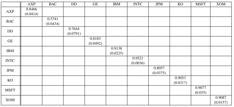
The following results were obtained when the model is applied to rotated data. Estimates of A˜ and

˜

B along with their standard errors are shown in Tables 1.1 and 1.2. The estimates of the unrotated parameters A and B are recovered according to (1.13). From the literature on GARCH models using realized measures, the variance/covariance process in this model is more responsive to innovations. As a result, the elements (in the diagonal positions) inA˜in (1.11) will be larger than those in traditional

2_{The ticker symbols are AXP(American Express), BAC(Bank of America), DD(DuPont), GE(General Electric), IBM,}

(36)

GARCH models. The means of the diagonal elements in the coefficient matrices are 0.722 forB˜ and 0.209 forA˜, which is in line with estimates found in other studies. The estimate forB˜ implies that the dynamic ofHtwill be smooth, though less smooth than the traditional GARCH model, which typically

(37)

Table 1.1: Parameter Estimates of the matrixA˜in the rotated RBEKK model

AXP BAC DD GE IBM INTC JPM KO MSFT XOM

AXP 0.5139 (0.0257)

BAC 0.8070

(0.0614)

DD 0.6297

(0.0652)

GE 0.5578

(0.034)

IBM 0.3817

(0.0097)

INTC 0.2727

(0.0008)

JPM 0.5759

(0.0272)

KO 0.4016

(0.0143)

MSFT 0.3961

(0.0155)

XOM 0.3938

(0.0072)

Table 1.2: Parameter Estimates of the matrixB˜in the rotated RBEKK model

AXP BAC DD GE IBM INTC JPM KO MSFT XOM

AXP 0.8466 (0.0414)

BAC 0.5741

(0.0434)

DD 0.7644

(0.0791)

GE 0.8183

(0.0492)

IBM 0.9138

(0.0225)

INTC 0.9521

(0.0036)

JPM 0.8057

(0.0375)

KO 0.9053

(0.0317)

MSFT 0.9077

(0.035)

XOM 0.9087

(38)

For the BEKK paramerization, using (1.13), the estimates ofAandB are

ˆ

A= ˆH¯1/2A˜Xˆ¯−1/2=                             

0.4620 0.1319 0.0567 0.0060 −0.0349 0.0286 −0.0222 −0.0029 −0.0068 0.0243

−0.0129 0.8201 0.0298 0.0048 −0.0646 0.0699 −0.0289 0.0261 0.0041 0.0030

0.0091 0.0535 0.5698 0.0103 −0.0369 0.0181 0.0039 0.0111 0.0154 0.0155

0.0008 0.0919 0.0480 0.4424 −0.0264 0.0679 −0.0168 0.0892 0.0484 0.0427

0.0107 0.0172 0.0358 0.0143 0.2984 0.0817 −0.0383 0.0583 0.0391 0.0439

0.0297 0.0417 0.0484 0.0223 0.0137 0.1994 −0.0643 0.0076 0.0351 0.0523

−0.0060 0.1748 0.0438 0.0159 −0.0207 0.0485 0.4628 0.0301 0.0128 0.0057

0.0126 0.0041 0.0188 0.0073 −0.0158 0.0800 −0.0471 0.3495 0.0641 0.0553

0.0118 0.0289 0.0336 0.0004 −0.0061 0.0917 −0.0453 0.0464 0.3390 0.0465

0.0173 0.0347 0.0403 0.0133 −0.0179 0.1451 −0.0586 0.0596 0.0810 0.3228                              ˆ

B= ˆH¯1/2B˜Hˆ¯−1/2=                             

0.8693 −0.0003 0.0132 0.0082 0.0020 −0.0210 0.0052 −0.0010 −0.0026 −0.0003

0.0008 0.4887 0.0231 0.0258 0.0065 −0.0543 0.0255 −0.0103 −0.0100 0.0070

−0.0074 −0.0085 0.7479 0.0087 −0.0033 −0.0208 0.0034 −0.0051 −0.0112 −0.0020

−0.0005 −0.0041 0.0190 0.8257 0.0076 −0.0672 0.0191 −0.0306 −0.0278 0.0006

0.0025 0.0034 0.0270 0.0378 0.9185 −0.0710 0.0173 −0.0136 −0.0235 0.0056

0.0216 0.0386 0.0167 0.0641 0.0489 0.9680 0.0438 0.0101 0.0143 0.0859

−0.0020 −0.0133 0.0147 0.0151 0.0032 −0.0449 0.8449 −0.0135 −0.0117 0.0035

0.0003 0.0069 0.0210 0.0722 0.0237 −0.0799 0.0288 0.9065 −0.0245 0.0148

0.0024 0.0070 0.0238 0.0497 0.0248 −0.0710 0.0194 −0.0019 0.9109 0.0276

0.0085 0.0089 0.0256 0.0546 0.0266 −0.1012 0.0226 −0.0061 −0.0243 0.9163                             

Asymmetry in A and B is typical with rotated models. The standard error of the estimates ofAandB can be obtained from the estimation of the rotated model using the delta method.

1.6.3 The ALasso method Under Different Selection Criteria

(39)

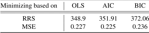
Since the OLS estimator is fully specified, this ranking should come as no surprise. OLS will generally obtain the best in-sample fit, while BIC-based shrinkage selects the most parsimonious model. The AIC-based shrinkage estimator has the smallest MSE since it balances the competing concerns of model fit and parsimony.

Table 1.3: Fit for Measurement Equation Estimators (1.8)

Minimizing based on OLS AIC BIC

RRS 348.9 351.91 372.06

MSE 0.227 0.225 0.236

Note theM SE =RSS/(N−K), whereN is the number

of observations andKis the number of variables.

(40)

Figure 1.1: ALasso shrinkage of the coefficients of the first measurement equation in (1.8).

(41)

Figure 1.3: Mean Squared Error ALasso as a function of relative model size

1.6.4 Estimation Results for the Measurement Equation

For the measurement equations, each realized variance (covariance) is a function of the corresponding conditional variance (covariance) and the conditional covariances of the pairs of all other assets (after taking the matrix logarithm). Assuming that there are three assets – A, B, and C – the realized vari-ance of asset A is updated by the conditional varivari-ance of A, and conditional covarivari-ance of A and B, the conditional covariance of A and C, and the conditional covariance of B and C. Each conditional variance/covariance is the main driver in updating its counterpart in the realized measure. As a result, the coefficient matrix should have larger elements in the diagonal positions. Most elements shrunk by the ALasso method are in the off-diagonal positions. Some diagonal elements will also shrink due to the nonlinear transformation by matrix logarithm reallocate the linkage between the corresponding elements in conditional variance/covariance matrix and realized kernel.

(42)

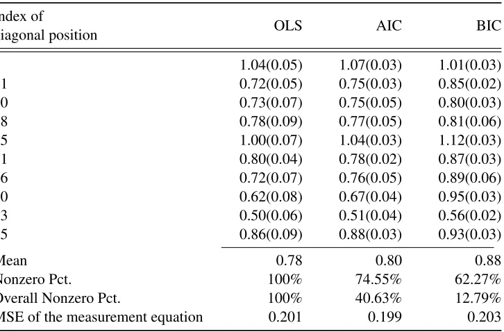
estimates of the matrix corresponding to the variance of each asset are compared under OLS and the ALasso method (AIC and BIC) estimation methods. In the last two rows, the percentage of non-zero coefficients in the matrixΓ, and the MSE, are given. As the OLS estimator does not shrink any variables, the percentage of non-zero coefficients is 100%. The number of non-zero coefficients under the AIC-based shrinkage estimator is 40.63%, much larger than the BIC-AIC-based shrinkage estimator’s 12.79%. Again, we find that BIC emphasizes the parsimony of the model. However, AIC is more accurate in terms of MSE. In the second to last row of the table, we show the number of non-zero elements on the diagonal of the coefficient matrix. The AIC-based shrinkage estimator results in 74.55% of the elements being zero, while the BIC-based estimator results in 67.27% of the elements being non-zero. The coefficient matrix estimated by the ALasso method is essentially a diagonal matrix with a high percentage of shrinkage occuring in off-diagonal positions. The fourth to last row of the table reports the mean of the coefficient for each variance. The value for BIC is 0.889, the largest of all the models, since this estimation method implies the most shrinkage.

To check the fit of the measurement equation, we focus on the test of autocorrelation of the residuals. If there are autocorrelation of residuals, we may need to add lags of dependent variables. The Lagrange multiplier (LM) test for autocorrelation developed by Breusch (1978) and Godfrey (1978) has become a standard tool in applied econometrics. It is often applied to the residuals of a multivariate regression such VAR or SUR of time series model. A vectorized version of LM test is proposed Doornik (1996) by testing the significance of lagged residualsuˆt−h(obtained under the null hypothesis) in the auxiliary

regression:

ut=d+ Γht+b1uˆt−1+...+bhuˆt−h+vt (1.24) vti.i.d∼ N(0,Σv)

We wish to test the significance of lagged residuals, so the null hypothesis is

(43)

Table 1.4: Estimates of coefficient matrixΓ

Index of

diagonal position OLS AIC BIC

1 1.04(0.05) 1.07(0.03) 1.01(0.03)

11 0.72(0.05) 0.75(0.03) 0.85(0.02)

20 0.73(0.07) 0.75(0.05) 0.80(0.03)

28 0.78(0.09) 0.77(0.05) 0.81(0.06)

35 1.00(0.07) 1.04(0.03) 1.12(0.03)

41 0.80(0.04) 0.78(0.02) 0.87(0.03)

46 0.72(0.07) 0.76(0.05) 0.89(0.06)

50 0.62(0.08) 0.67(0.04) 0.95(0.03)

53 0.50(0.06) 0.51(0.04) 0.56(0.02)

55 0.86(0.09) 0.88(0.03) 0.93(0.03)

Mean 0.78 0.80 0.88

Nonzero Pct. 100% 74.55% 62.27%

Overall Nonzero Pct. 100% 40.63% 12.79%

MSE of the measurement equation 0.201 0.199 0.203

Estimates of the coefficient matrixΓof the measurement equation under OLS and ALasso

using AIC and BIC criteria. The numbers in parentheses are standard errors. The Nonzero Pct means the percentage of nonzero estimates in the diagonal position of coefficient matrix

Γ. The Overall Nonzero Pct means the percentage of nonzero estimates of all position in

(44)

which implies no autocorrelation of residuals for lag one through lagh. The test statistic is constructed as:

LM =T nR2_m (1.26)

with an asymptoticχ2_hn2 under null .nis the dimension of the system,h is the number added lagged

regressors in the each auxiliary regression and T is the sample size. R2_m is aR2-type measures of goodness of fit:

R2_m= 1−(1/n)tr(ˆvvˆ0)(ˆuuˆ0) (1.27)

where v and u arep∗byTmatrix of residuals from the auxiliary regressions and measurement equations. Since the dimension is large relative to the sample size, we only test the lag for 2. LM value for the measurement equation with OLS and LASSO are 5717 and 2421, and the p-value are 0.999 and 1, which can’t reject the null hypothesis.

1.7 Model predictive Ability Evaluation

We compare the out-of-sample performance of the ALasso method and OLS, when estimating the mea-surement equation. Let the loss function Lt,s(Ht0+s,Hˆti+s|t) denote the loss at time t resulting from

thes-step ahead forecast using modeli. Under this notation,H_t0₊_s denotes the true (latent) covariance matrix and Hˆ_ti₊_s_|_t is thes-step ahead forecast of modeli conditional on the information set at time t. Since the latent covariance H_t0₊_s is unobservable, we use the realized kernel as a proxy such that

ˆ

H_t0₊_s=Xt+s. We use the quasi-likelihood (QLIK) loss function:

t+s). (1.28)

(45)

is robust to noise in the proxy realized measureXt+s(Patton and Sheppard, 2009; Laurent, Rombouts,

and Violante, 2013).

Denote the total sample size by is T, dividing it into Tin of in-sample andTout of out-of-sample

portions. ThenTout−s+ 1is the number of s-step ahead predictions, the out-of-sample observations

spanTin+sthroughTin+Tout. The estimation window (in-sample) portion runs from January 4, 2006

to April 29, 2011 with a sample size of 1340. The out-of-sample portion runs from May 2, 2011 to April 30, 2012 with a sample size of 252. Given the loss function, the loss difference is

Dt,s=Lt,s( ˆHt0+s|t,Hˆ Lasso

t+s|t )−Lt,s( ˆHt0+s|t,Hˆ OLS t+s|t),

t=Tin, Tin+ 1, ..., T−s.

The average loss is then

¯

Ds=

1 (Tout−s+ 1)

T−s+1 X

t=Tin

Dt,s. (1.29)

Average loss was used in tests of predictive ability by Diebold and Mariano (1995) and West (1996). The null and alternative hypotheses are

H0 :E[Dt,s] = 0,

H1 :E[Dt,s]>0,

or H2 :E[Dt,s]<0.

The test statistic is constructed as

Tloss= (Tout−s+ 1)1/2 ¯

Ds ˆ

S_d1/2

(46)

where

ˆ

Sd= s

X

j=−s ˆ

τ(j),

ˆ

τ(j) = ˆτ(−j) = (Tout−s+ 1)−1 T−s+1

X

t=Tin

(Dt−j,s−D¯s)(Dt,s−D¯s),

j= 1,2, ..., s.

Significantly negative values of the test statistic indicate that the measurement equation estimated with the ALasso method has superior forecast performance compared to the OLS estimate. The test of fore-cast ability is conducted on the rotated model using two different estimators for the measurement equa-tions. We estimate the model with an expanding window (recursively), starting from observation number 1342, and then use the parameter estimates to obtain forecasts ofHtat horizonss= 1,2,3, ...,22days.

The parameters are updated every 5 days, so the expanding window grows by 5. The estimation and prediction are repeated 50 and 250 times respectively.

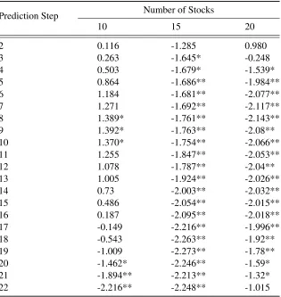
Results for the test are given in Table 1.5. The results for 10 assets show that the difference in loss function is statistically significant and positive at the 10% level at horizons s = 8,9,10. The difference is statistically significant and negative at the 10% level at horizon s = 20and at the 5% level at horizonss= 21,22. The results with 15 stocks3 show significantly negative values at the 10% significance level at horizonss= 3,4and at the 5% significance level at horizonss= 5,6, ...,22. With 20 stocks,4significantly negative values occur at the 10% significance level at horizonss= 4,20,21and at the 5% significance level at horizonss= 5,6, ...,19. Broadly, the measurement equation estimated with the ALasso method outperforms the measurement equation estimated with OLS. The difference in performance between the two estimators increases as the number of assets under consideration increases. The statisticsD¯sshow improvement in the 15 and 20 stock cases, except at the far end of the forecast

horizon. The advantageous predictive power of the ALasso method in the 20 stock case is diminished at long forecasting horizons. Overall, the model using the ALasso method performs significantly better

3

(47)

than OLS methods, and this effect is more pronounced when additional assets are considered.

Table 1.5: Statistical Test of Predictive Ability

Prediction Step Number of Stocks

10 15 20

2 0.116 -1.285 0.980

3 0.263 -1.645* -0.248

4 0.503 -1.679* -1.539*

5 0.864 -1.686** -1.984**

6 1.184 -1.681** -2.077**

7 1.271 -1.692** -2.117**

8 1.389* -1.761** -2.143**

9 1.392* -1.763** -2.08**

10 1.370* -1.754** -2.066**

11 1.255 -1.847** -2.053**

12 1.078 -1.787** -2.04**

13 1.005 -1.924** -2.026**

14 0.73 -2.003** -2.032**

15 0.486 -2.054** -2.015**

16 0.187 -2.095** -2.018**

17 -0.149 -2.216** -1.996**

18 -0.543 -2.263** -1.92**

19 -1.009 -2.273** -1.78**

20 -1.462* -2.246** -1.59*

21 -1.894** -2.213** -1.32*

22 -2.216** -2.248** -1.015

Test of predictive ability: Loss(ALasso)-Loss(OLS). A negative test value indi-cates model using the ALasso method has better predictive ability. The critical values are: 2.4 (1%), 1.68 (5%), 1.3 (10%). * denotes significance at the 10% level, ** significance at the 5% level, and *** significance at the 1% level

(48)

as:

Lt,s( ˆHt0+s, Hti+s|t) = 1/N2 N

X

m,n=1

(h(mn)i_t₊_s_|_t−ˆh(mn)0_t₊_s)2. (1.31)

whereh(mn)i_t₊_s_|_t is the element in mthrow andnthcolumn in H_ti₊_s_|_t, similar definition goes with

ˆ

hmn

0

t+s. Comparing (1.28) with (1.31), the former loss function represents which method are more

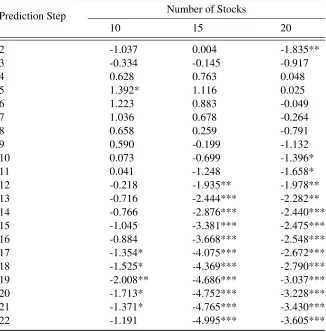
possibly predict the true covariance the later indicate which method is closer to the true covariance with respect of the estimated value. The result of portfolio with 10, 15 and 20 assets for each forecast step are reported in Table 1.6. From the table, we can see that the mode with Alasso performs better for the portfolio with more number of assets and for the further steps in forecasting. Further, we can check the economical difference by inserting these predictive covariances into asset pricing formula or calculating the Value at risk.

1.8 Conclusion

(49)

Table 1.6: Gain of predictive covariance using ALasso

Prediction Step Number of Stocks

10 15 20

2 -1.037 0.004 -1.835**

3 -0.334 -0.145 -0.917

4 0.628 0.763 0.048

5 1.392* 1.116 0.025

6 1.223 0.883 -0.049

7 1.036 0.678 -0.264

8 0.658 0.259 -0.791

9 0.590 -0.199 -1.132

10 0.073 -0.699 -1.396*

11 0.041 -1.248 -1.658*

12 -0.218 -1.935** -1.978**

13 -0.716 -2.444*** -2.282**

14 -0.766 -2.876*** -2.440***

15 -1.045 -3.381*** -2.475***

16 -0.884 -3.668*** -2.548***

17 -1.354* -4.075*** -2.672***

18 -1.525* -4.369*** -2.790***

19 -2.008** -4.686*** -3.037***

20 -1.713* -4.752*** -3.228***

21 -1.371* -4.765*** -3.430***

22 -1.191 -4.995*** -3.605***

(50)

Chapter 2

Realized Markov Regime-Switching

BEKK Model

2.1 Introduction

In the last few decades, GARCH (Generalized Autoregressive Conditional Heteroscedasticity) models, which were introduced by Engle (1982) and Bollerslev (1986) have been the most popular and successful models in characterizing financial volatility. However, GARCH models often give good in-sample fit, but poor out-of-sample forecasting performance. According to Andersen and Bollerslev (1998), one reason for this is we typically compare the model forecasts with a weak measure of ex-post volatility, such as squared returns. The solution is to use the “realized volatility” calculated with intra-daily data. The other common problem of GARCH models in forecasting is that the volatility forecasts are usually too smooth and too high across periods due to structure breaks. Hamilton and Susmel (1994), for example, found that, for their stock return data, a shock on a given week would produce non-negligible effects on the variance more than one year later. Lamoureux and Lastrapes (1990), among others, show that this persistence may originate from structural changes in the variance process.

(51)

to forecasts that are far from realizations (see Stock and Watson, 1996). The accumulated evidence from empirical research suggests that the volatility of financial markets displays a type of persistence that cannot be appropriately explained by classical GARCH models. In particular, these models usually show high persistence in the conditional volatility which is not compatible with the poor out-of-sample forecasting results of these models. These findings indicate a potential source of misspecification in that the structural form of the conditional mean and variance is relatively inflexible and fixed throughout the entire sampling period. Therefore, models in which the parameters are allowed to change over time may be more appropriate for modeling volatility.

Since the seminal paper by Hamilton (1989), which characterized the U.S. business cycle by pe-riodic shifts from recessions to expansions and vice versa, the use of Markov-switching models has become increasingly popular in dynamic econometrics. The dynamics of the observed process is driven by a standard GARCH model as long as the persistence mechanism remains in the same regime and is powered by a different standard GARCH model whenever the working mechanism switches to an-other regime. Introducing change in the regime increases the model flexibility substantially and allows for interesting economic interpretations. See Kaufmann and Scheicher (1996) for a survey on Markov-switching models.

In the present work, we incorporate a GARCH model into a Markov regime-switching framework to allow for different volatility regimes. Within each regime, we use a GARCH model to govern the variance. The persistence of both regimes yields an extra source of volatility persistence compared with standard, single-regime GARCH, thereby enhancing the flexibility in describing the volatility persis-tence of shocks.

(52)

(2002) also integrates out the unobserved regimes, using all available information up to timet, whereas Gray (1996) only integrates conditional on information up tot−1. By doing so, the model becomes path-independent and the likelihood is tractable even with a large sample size.

Our realized Markov regime-switching GARCH model is as an extension of Klaassen’s (2002) univariate generalized Markov regime-switching model to the bivariate case (except the forecasting mechanism) and potentially multiple-variate case. To improve not only the out-of-sample forecasting performance but also the accuracy of forecast evaluation, we use the realized measure as the ex-post volatility. In our model, a latent state variable governing the regime shifts follows a first-order, two-state Markov process, the parameters of which are estimated via quasi-maximum likelihood along with other unknown parameters, including transition probability and prediction probability of regimes.

2.2 The Markov Regime-Switching GARCH Model

The basic set up of the univariate Markov Regime-Switching GARCH Model is shown in this section. Letptbe the price of a financial asset at the end of day t, then definert = log(pt)−log(pt−1)as the daily return. Letst be the unobserved variance regime at timet, which represents different state

of volatility dynamics. Note that the time subscript t of the expectation operator Et and probability pt means the arguments are conditional on some information sets, e.g. pt(x) = p(x|Ft), in which

Ft represents the observable information set till period t, and we use the notation pt−1(st|s˜t−1) = p(st|Ft−1,s˜t−1)to denote the ex-ante probability of some series going to regimestat a specific timet

conditional on the information set of the data-generating process, which consists of two parts. The first part,F_t−1, denotes the information that can be observed, which is(rt−1, rt−2,· · ·, r1)in our case. The second part,s˜t−1, is the regime path(st−1, st−2,· · · , s1), which can not be observed. The dynamic of the conditional variance of return,h˜st,t=vart−1(rt|s˜t), is our research interest, where the subscription

t, stofhmeans the conditional variance predicted for timetbased on the information set including the

(53)

Markov process with constant transition probabilities independent with time stamptdefined as:

pij =p(st=j|st−1 =i) (2.1)

withpt,i1 +pt,i2 = 1fori, j = 1,2.Equation (2.1) indicates the probability of switching from statei at timet−1 to statejatt. The transition probability matrix is a2by 2matrix composed with these probabilities

P =

  

p11 p12

p21 p22   =

  

p11 1−p11

1−p22 p22  

 (2.2)

The unconditional probability of staying in statest= 1is equal toπ1 = (1−p11)/(2−p11−p22). We choose to model the mean of the daily return as zero since the focus of this paper is the volatility rather than the mean. If the mean of daily return is not zero, it would also typically be modeled as a Markov regime-switching quantity, but not bring much change to our structure. Therefore, under the full regime path-dependent specification, the return equation is modeled as

rt=h1_s_˜/_t_,t2zt (2.3) zti.i.d∼ (0,1)

where ht,˜st = vart(rt|It−1,s˜t) denotes the time-varying state-dependent variance given the whole

regime path. The Markov regime-switching conditional covariancehs˜t,tfollows a GARCH(1,1) process:

h˜st,t=ωst +bstht−1,s˜t−1 +astr

2

t−1.