Bayesian Inference for Finite-State Transducers
∗David Chiang1 Jonathan Graehl1 Kevin Knight1 Adam Pauls2 Sujith Ravi1
1Information Sciences Institute
University of Southern California 4676 Admiralty Way, Suite 1001
Marina del Rey, CA 90292
2Computer Science Division
University of California at Berkeley Soda Hall
Berkeley, CA 94720
Abstract
We describe a Bayesian inference algorithm that can be used to train any cascade of weighted finite-state transducers on end-to-end data. We also investigate the problem of automatically selecting from among mul-tiple training runs. Our experiments on four different tasks demonstrate the genericity of this framework, and, where applicable, large improvements in performance over EM. We also show, for unsupervised part-of-speech tagging, that automatic run selection gives a large improvement over previous Bayesian ap-proaches.
1 Introduction
In this paper, we investigate Bayesian infer-ence for weighted finite-state transducers (WFSTs). Many natural language models can be captured by weighted finite-state transducers (Pereira et al., 1994; Sproat et al., 1996; Knight and Al-Onaizan, 1998; Clark, 2002; Kolak et al., 2003; Mathias and
Byrne, 2006), which offer several benefits:
• WFSTs provide a uniform knowledge
represen-tation.
• Complex problems can be broken down into a
cascade of simple WFSTs.
• Input- and output-epsilon transitions allow
compact designs.
• Generic algorithms exist for doing inferences
with WFSTs. These include best-path
de-coding, k-best path extraction, composition,
∗
The authors are listed in alphabetical order. Please direct correspondence to Sujith Ravi ([email protected]). This work was supported by NSF grant IIS-0904684 and DARPA contract HR0011-06-C0022.
intersection, minimization, determinization, forward-backward training, forward-backward pruning, stochastic generation, and projection.
• Software toolkits implement these generic
al-gorithms, allowing designers to concentrate on novel models rather than problem-specific in-ference code. This leads to faster scientific ex-perimentation with fewer bugs.
Weighted tree transducers play the same role for problems that involve the creation and transforma-tion of tree structures (Knight and Graehl, 2005). Of course, many problems do not fit either the finite-state string or tree transducer framework, but in this paper, we concentrate on those that do.
Bayesian inference schemes have become popu-lar recently in natural language processing for their ability to manage uncertainty about model param-eters and to allow designers to incorporate prior knowledge flexibly. Task-accuracy results have gen-erally been favorable. However, it can be time-consuming to apply Bayesian inference methods to each new problem. Designers typically build cus-tom, problem-specific sampling operators for ex-ploring the derivation space. They may factor their programs to get some code re-use from one problem to the next, but highly generic tools for string and tree processing are not available.
In this paper, we marry the world of finite-state machines with the world of Bayesian inference, and we test our methods across a range of natural lan-guage problems. Our contributions are:
• We describe a Bayesian inference algorithm
that can be used to train any cascade of WFSTs on end-to-end data.
• We propose a method for automaticrun
tion, i.e., how to automatically select among multiple training runs in order to achieve the best possible task accuracy.
The natural language applications we consider in this paper are: (1) unsupervised part-of-speech (POS) tagging (Merialdo, 1994; Goldwater and
Griffiths, 2007), (2) letter substitution
decipher-ment (Peleg and Rosenfeld, 1979; Knight et al., 2006; Ravi and Knight, 2008), (3) segmentation of space-free English (Goldwater et al., 2009), and (4)
Japanese/English phoneme alignment (Knight and
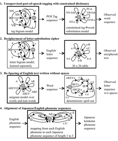
Graehl, 1998; Ravi and Knight, 2009a). Figure 1 shows how each of these problems can be repre-sented as a cascade of finite-state acceptors (FSAs) and finite-state transducers (FSTs).
2 Generic EM Training
We first describe forward-backward EM training for
a single FST M. Given a string pair (v,w) from our
training data, we transform v into an FST Mv that
just maps vto itself, and likewise transform winto
an FSTMw. Then we composeMvwithM, and
com-pose the result with Mw. This composition follows
Pereira and Riley (1996), treating epsilon input and output transitions correctly, especially with regards to their weighted interleaving. This yields a
deriva-tion latticeD, each of whose paths transformsvinto
w.1 Each transition inDcorresponds to some
tran-sition in the FST M. We run the forward-backward
algorithm overDto collect fractional counts for the
transitions inM. After we sum fractional counts for
all examples, we normalize with respect to
com-peting transitions in M, assign new probabilities to
M, and iterate. Transitions in Mcompete with each
other if they leave the same state with the same input
symbol, which may be empty ().
In order to train an FSA on observed string data, we convert the FSA into an FST by adding an input-epsilon to every transition. We then convert each
training stringvinto the string pair (,v). After
run-ning the above FST trairun-ning algorithm, we can
re-move all input-from the trained machine.
It is straightforward to modify generic training to support the following controls:
1Throughout this paper, we do not assume that lattices are
acyclic; the algorithms described work on general graphs.
B:E
a:A b:B A:D A:C
=
a:
:D
:E b:
[image:2.612.352.503.59.152.2]a: :C
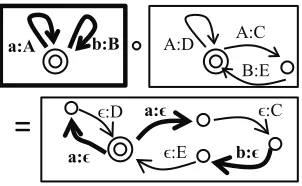
Figure 2: Composition of two FSTs maintaining separate transitions.
Maximum iterations and early stopping.We
spec-ify a maximum number of iterations, and we halt
early if the ratio of logP(data) from one iteration
to the next exceeds a threshold (such as 0.99999).
Initial point.Any probabilities supplied on the
pre-trained FST are interpreted as a starting point for EM’s search. If no probabilities are supplied, EM begins with uniform probabilities.
Random restarts.We can requestnrandom restarts,
each from a different, randomly-selected initial
point.
Locking and tying. Transitions on the pre-trained
FST can be marked as locked, in which case EM will not modify their supplied probabilities. Groups of transitions can be tied together so that their frac-tional counts are pooled, and when normalization occurs, they all receive the same probability.
Derivation lattice caching.If memory is available,
training can cache the derivation lattices computed in the first EM iteration for all training pairs. Subse-quent iterations then run much faster. In our experi-ments, we observe an average 10-fold speedup with caching.
Next we turn to training a cascade of FSTs on
end-to-end data. The algorithm takes as input: (1) a sequence of FSTs, and (2) pairs of training strings
(v,w), such that v is accepted by the first FST in
the cascade, andwis produced by the last FST. The
algorithm outputs the same sequence of FSTs, but with trained probabilities.
To accomplish this, we first compose the supplied
FSTs, taking care to keep the transitions from diff
prob-ABCD:a REY:r
!:c
1. Unsupervised part-of-speech tagging with constrained dictionary
POS Tag sequence
Observed word sequence
2. Decipherment of letter-substitution cipher
English letter sequence
Observed enciphered text
3. Re-Spacing of English text written without spaces
Word sequence
Observed letter sequence w/o spaces
4. Alignment of Japanese/English phoneme sequences
English phoneme sequence
Japanese katakana phoneme sequence 26 x 26 table letter bigram model,
learned separately
constrained tag!word substitution model tag bigram model
unigram model over
words and non-words deterministic spell-out
mapping from each English phoneme to each Japanese phoneme sequence of length 1 to 3 NN
JJ JJ JJ NN
VB !
!
!
NN:fish
IN:at VB:fish
SYM:a DT:a
a
b b b a
c !
!
! a:A
a:B a:C
b:A b:B b:C
A AR
ARE AREY AREYO
!:!
AREY:a
!:b
!:d
!:r !:e
!:y
AE:!
!:S
!:S
[image:3.612.115.498.143.602.2]!:U
abilities are tied together. Next, we run FST train-ing on the end-to-end data. This involves creattrain-ing derivation lattices and running forward-backward on them. After FST training, we de-compose the trained device back into a cascade of trained machines.
When the cascade’s first machine is an FSA, rather than an FST, then the entire cascade is viewed as a generator of strings rather than a transformer of strings. Such a cascade is trained on observed strings rather than string pairs. By again treating the first FSA as an FST with empty input, we can train using the FST-cascade training algorithm described in the previous paragraph.
Once we have our trained cascade, we can apply it
to new data, obtaining (for example) thek-best
out-put strings for an inout-put string.
3 Generic Bayesian Training
Bayesian learning is a wide-ranging field. We focus on training using Gibbs sampling (Geman and Ge-man, 1984), because it has been popularly applied in the natural language literature, e.g., (Finkel et al., 2005; DeNero et al., 2008; Blunsom et al., 2009).
Our overall plan is to give a generic algorithm for Bayesian training that is a “drop-in replacement” for EM training. That is, we input an FST cas-cade and data and output the same FST cascas-cade with trained weights. This is an approximation to a purely Bayesian setup (where one would always in-tegrate over all possible weightings), but one which
makes it easy to deploy FSTs to efficiently decode
new data. Likewise, we do not yet support non-parametric approaches—to create a drop-in replace-ment for EM, we require that all parameters be spec-ified in the initial FST cascade. We return to this is-sue in Section 5.
3.1 Particular Case
We start with a well-known application of Bayesian inference, unsupervised POS tagging (Goldwater
and Griffiths, 2007). Raw training text is provided,
and each potential corpus tagging corresponds to a hidden derivation of that data. Derivations are cre-ated and probabilistically scored as follows:
1. i←1
2. Choose tagt1according toP0(t1)
3. Choose wordw1according toP0(w1|t1)
4. i←i+1
5. Choose tagti according to
αP0(ti |ti−1)+ci1−1(ti−1,ti) α+ci1−1(ti−1)
(1)
6. Choose wordwiaccording to
βP0(wi |ti)+ci1−1(ti,wi) β+ci1−1(ti)
(2)
7. With probabilityPquit, quit; else go to 4.
This defines the probability of any given derivation.
The base distribution P0 represents prior
knowl-edge about the distribution of tags and words, given
the relevant conditioning context. The ci1−1 are the
counts of events occurring before word i in the
derivation (the “cache”).
Whenαandβare large, tags and words are
essen-tially generated according toP0. Whenαandβare
small, tags and words are generated with reference to previous decisions inside the cache.
We use Gibbs sampling to estimate the
distribu-tion of tags given words. The key to efficient
sam-pling is to define a samsam-pling operator that makes some small change to the overall corpus derivation. With such an operator, we derive an incremental formula for re-scoring the probability of an entire new derivation based on the probability of the old
derivation. Exchangeability makes this efficient—
we pretend like the area around the small change oc-curs at the end of the corpus, so that both old and new derivations share the same cache. Goldwater
and Griffiths (2007) choose the re-sampling operator
“change the tag of a single word,” and they derive the corresponding incremental scoring formula for unsupervised tagging. For other problems,
design-ers develop different sampling operators and derive
different incremental scoring formulas.
3.2 Generic Case
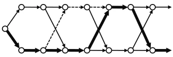
Figure 3: Changing a decision in the derivation lattice. All paths generate the observed data. The bold path rep-resents the current sample, and the dotted path reprep-resents a sidetrack in which one decision is changed.
compute derivation lattices for our observed training data through our cascade of FSTs. A random path through these lattices constitutes the initial sample, and we calculate its derivation probability directly.
One way to think about a generic small change operator is to consider a single transition in the cur-rent sample. This transition will generally compete with other transitions. One possible small change is to “sidetrack” the derivation to a competing deriva-tion. Figure 3 shows how this works. If the sidetrack path quickly re-joins the old derivation path, then an incremental score can be computed. However, side-tracking raises knotty questions. First, what is the proper path continuation after the sidetracking tran-sition is selected? Should the path attempt to re-join the old derivation as soon as possible, and if so, how
is this efficiently done? Then, how can we compute
new derivation scores for all possible sidetracks, so that we can choose a new sample by an appropriate weighted coin flip? Finally, would such a sampler be reversible? In order to satisfy theoretical conditions
for Gibbs sampling, if we move from sample Ato
sampleB, we must be able to immediately get back
to sampleA.
We take a different tack here, moving from
point-wise sampling to blocked sampling. Gao and John-son (2008) employed blocked sampling for POS tag-ging, and the approach works nicely for arbitrary derivation lattices. We again start with a random derivation for each example in the corpus. We then choose a training example and exchange its entire derivation lattice to the end of the corpus. We
cre-ate a weighted version of this lattice, called the
pro-posal lattice, such that we can approximately sample whole paths by stochastic generation. The probabil-ities are based on the event counts from the rest of the sample (the cache), and on the base distribution,
and are computed in this way:
P(r|q)= αP0(rα|q)+c(q,r)
+c(q) (3)
whereqandrare states of the derivation lattice, and
thec(·) are counts collected from the corpus minus
the entire training example being resampled. This is an approximation because we are ignoring the fact
that P(r | q) in general depends on choices made
earlier in the lattice. The approximation can be cor-rected using the Metropolis-Hastings algorithm, in which the sample drawn from the proposal lattice is
accepted only with a certain probabilityα; but Gao
and Johnson (2008) report thatα >0.99, so we skip
this step.
3.3 Choosing the best derivations
After the sampling run has finished, we can choose
the best derivations using two different methods.
First, if we want to find the MAP derivations of the training strings, then following Goldwater and
Grif-fiths (2007), we can useannealing: raise the
proba-bilities in the sampling distribution to the T1 power,
whereT is a temperature parameter, decreaseT
to-wards zero, and take a single sample.
But in practice one often wants to predict the
MAP derivation for a new string w0 not contained
in the training data. To approximate the distribution
of derivations ofw0given the training data, we
aver-age the transition counts from all the samples (after burn-in) and plug the averaged counts into (3) to
ob-tain a single proposal lattice.2The predicted
deriva-tion is the Viterbi path through this lattice. Call this
methodaveraging. An advantage of this approach is
that the trainer, taking a cascade of FSAs as input, outputs a weighted version of the same cascade, and this trained cascade can be used on unseen examples without having to rerun training.
3.4 Implementation
That concludes the generic Bayesian training algo-rithm, to which we add the following controls:
2A better approximation might have been to build a proposal
Number of Gibbs sampling iterations.We execute the full number specified.
Base distribution.Any probabilities supplied on the
pre-trained FST are interpreted as base distribution probabilities. If no probabilities are supplied, then the base distribution is taken to be uniform.
Hyperparameters.We supply a distinctαfor each
machine in the FST cascade. We do not yet support differentαvalues for different states within a single FST.
Random restarts. We can request multiple runs
from different, randomly-selected initial samples.
EM-based initial point. If random initial samples
are undesirable, we can request that the Gibbs sam-pler be initialized with the Viterbi path using
param-eter values obtained byniterations of EM.
Annealing schedule.If annealing is used, it follows
a linear annealing schedule with starting and stop-ping temperature specified by the user.
EM and Bayesian training for arbitrary FST cascades are both implemented in the finite-state toolkit Carmel, which is distributed with source
code.3 All controls are implemented as
command-line switches. We use Carmel to carry out the exper-iments in the next section.
4 Run Selection
For both EM and Bayesian methods, different
train-ing runs yield different results. EM’s objective
func-tion (probability of observed data) is very bumpy for
the unsupervised problems we work on—different
initial points yield different trained WFST cascades,
with different task accuracies. Averaging task
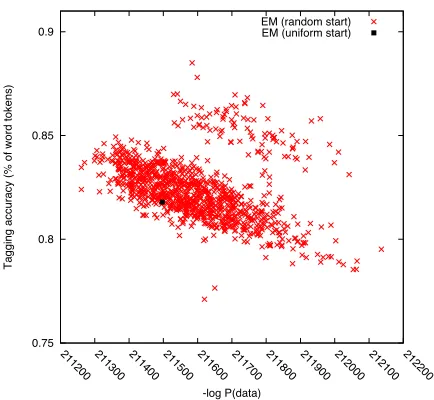
accu-racies across runs is undesirable, because we want to deploy a particular trained cascade in the real world, and we want an estimate of its performance. Select-ing the run with the best task accuracy is illegal in an unsupervised setting. With EM, we have a good al-ternative: select the run that maximizes the objective function, i.e., the likelihood of the observed training data. We find a decent correlation between this value and task accuracy, and we are generally able to im-prove accuracy using this run selection method. Fig-ure 4 shows a scatterplot of 1000 runs for POS tag-ging. A single run with a uniform start yields 81.8%
3http://www.isi.edu/licensed-sw/carmel
0.75 0.8 0.85 0.9
211200 211300 211400 211500 211600 211700 211800 211900 212000 212100 212200
Tagging accuracy (% of word tokens)
-log P(data)
[image:6.612.316.533.64.264.2]EM (random start) EM (uniform start)
Figure 4: Multiple EM restarts for POS tagging. Each point represents one random restart; the y-axis is tag-ging accuracy and thex-axis is EM’s objective function, −logP(data).
accuracy, while automatic selection from 1000 runs yields 82.4% accuracy.
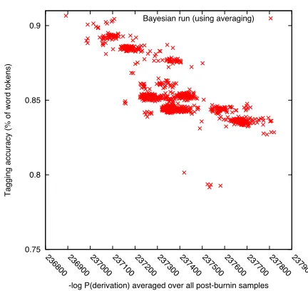
Gibbs sampling runs also yield WFST cascades with varying task accuracies, due to random initial samples and sampling decisions. In fact, the varia-tion is even larger than what we find with EM. It is natural to ask whether we can do automatic run se-lection for Gibbs sampling. If we are using anneal-ing, it makes sense to use the probability of the fi-nal sample, which is supposed to approximate the MAP derivation. When using averaging, however, choosing the final sample would be quite arbitrary. Instead, we propose choosing the run that has the highest average log-probability (that is, the lowest entropy) after burn-in. The rationale is that the runs that have found their way to high-probability peaks are probably more representative of the true distri-bution, or at least capture a part of the distribution that is of greater interest to us.
0.75 0.8 0.85 0.9
235100 235150 235200 235250 235300 235350 235400
Tagging accuracy (% of word tokens)
[image:7.612.317.533.66.270.2]-log P(derivation) for final sample Bayesian run (with annealing)
Figure 5: Multiple Bayesian learning runs (using anneal-ingwith temperature decreasing from 2 to 0.08) for POS tagging. Each point represents one run; they-axis is tag-ging accuracy and thex-axis is the−logP(derivation) of the final sample.
0.75 0.8 0.85 0.9
236800 236900 237000 237100 237200 237300 237400 237500 237600 237700 237800 237900
Tagging accuracy (% of word tokens)
-log P(derivation) averaged over all post-burnin samples Bayesian run (using averaging)
Figure 6: Multiple Bayesian learning runs (using averag-ing) for POS tagging. Each point represents one run; the
y-axis is tagging accuracy and the x-axis is the average −logP(derivation) over all samples after burn-in.
Bayesian methods (85.2% from Goldwater and Grif-fiths (2007), who use a trigram model) and close to the best accuracy reported on this task (91.8% from Ravi and Knight (2009b), who use an integer linear program to minimize the model directly).
5 Experiments and Results
We run experiments for various natural language ap-plications and compare the task accuracies achieved by the EM and Bayesian learning methods. The tasks we consider are:
Unsupervised POS tagging. We adopt the
com-mon problem formulation for this task described by Merialdo (1994), in which we are given a raw 24,115-word sequence and a dictionary of legal tags for each word type. The tagset consists of 45 dis-tinct grammatical tags. We use the same modeling
approach as as Goldwater and Griffiths (2007),
us-ing a probabilistic tag bigram model in conjunction with a tag-to-word model.
Letter substitution decipherment. Here, the task
is to decipher a 414-letter substitution cipher and un-cover the original English letter sequence. The task accuracy is defined as the percent of ciphertext
to-kens that are deciphered correctly. We work on the same standard cipher described in previous litera-ture (Ravi and Knight, 2008). The model consists of an English letter bigram model, whose probabil-ities are fixed and an English-to-ciphertext channel model, which is learnt during training.
Segmentation of space-free English. Given
a space-free English text corpus (e.g.,
iwalkedtothe...), the task is to segment the
text into words (e.g., i walked to the ...).
Our input text corpus consists of 11,378 words, with spaces removed. As illustrated in Figure 1, our method uses a unigram FSA that models every letter sequence seen in the data, which includes both words and non-words (at most 10 letters long) composed with a deterministic spell-out model. In order to evaluate the quality of our segmented output, we compare it against the gold segmentation and compute the word token f-measure.
Japanese/English phoneme alignment. We
use the problem formulation of Knight and
Graehl (1998). Given an input English/Japanese
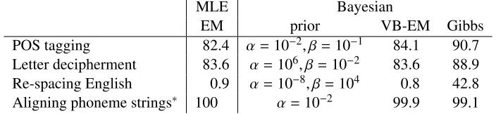
[image:7.612.76.292.71.270.2]MLE Bayesian
EM prior VB-EM Gibbs
POS tagging 82.4 α=10−2, β=10−1 84.1 90.7
Letter decipherment 83.6 α=106, β=10−2 83.6 88.9
Re-spacing English 0.9 α=10−8, β=104 0.8 42.8
[image:8.612.130.482.62.143.2]Aligning phoneme strings∗ 100 α=10−2 99.9 99.1
Table 1: Gibbs sampling for Bayesian inference outperforms both EM and Variational Bayesian EM.∗The output of EM alignment was used as the gold standard.
phoneme to its corresponding Japanese sounds (a sequence of one or more Japanese phonemes). For
example, given a phoneme sequence pair ((AH B
AW T) → (a b a u t o)), we have to produce
the alignments ((AH → a), (B → b), (AW →
a u), (T → t o)). The input data consists of
2,684 English/Japanese phoneme sequence pairs.
We use a model that consists of mappings from each English phoneme to Japanese phoneme sequences (of length up to 3), and the mapping probabilities are learnt during training. We manually analyzed the alignments produced by the EM method for this task and found them to be nearly perfect. Hence, for the purpose of this task we treat the EM alignments as our gold standard, since there are no gold alignments available for this data.
In all the experiments reported here, we run EM for 200 iterations and Bayesian for 5000 iterations (the first 2000 for burn-in). We apply automatic run selection using the objective function value for EM and the averaging method for Bayesian.
Table 1 shows accuracy results for our four tasks, using run selection for both EM and Bayesian learn-ing. For the Bayesian runs, we compared two infer-ence methods: Gibbs sampling, as described above, and Variational Bayesian EM (Beal and Ghahra-mani, 2003), both of which are implemented in
Carmel. We used the hyperparameters (α, β) as
shown in the table. Setting a high value yields a
fi-nal distribution that is close to the origifi-nal one (P0).
For example, in letter decipherment we want to keep the language model probabilities fixed during train-ing, and hence we set the prior on that model to
be very strong (α = 106). Table 1 shows that the
Bayesian methods consistently outperform EM for all the tasks (except phoneme alignment, where EM was taken as the gold standard). Each iteration of
Gibbs sampling was 2.3 times slower than EM for POS tagging, and in general about twice as slow.
6 Discussion
We have described general training algorithms for FST cascades and their implementation, and exam-ined the problem of run selection for both EM and Bayesian training. This work raises several interest-ing points for future study.
First, is there an efficient method for
perform-ing pointwise samplperform-ing on general FSTs, and would pointwise sampling deliver better empirical results than blocked sampling across a range of tasks?
Second, can generic methods similar to the ones described here be developed for cascades of tree transducers? It is straightforward to adapt our meth-ods to train a single tree transducer (Graehl et al., 2008), but as most types of tree transducers are not closed under composition (G´ecseg and Steinby,
1984), the compose/de-compose method cannot be
directly applied to train cascades.
Third, what is the best way to extend the FST for-malism to represent non-parametric Bayesian mod-els? Consider the English re-spacing application. We currently take observed (un-spaced) data and build a giant unigram FSA that models every letter se-quence seen in the data of up to 10 letters, both words and non-words. This FSA has 207,253
tran-sitions. We also defineP0for each individual
transi-tion, which allows a preference for short words. This set-up works fine, but in a nonparametric approach,
P0 is defined more compactly and without a
References
Matthew J. Beal and Zoubin Ghahramani. 2003. The Variational Bayesian EM algorithm for incomplete data: with application to scoring graphical model structures. Bayesian Statistics, 7:453–464.
Phil Blunsom, Trevor Cohn, Chris Dyer, and Miles Os-borne. 2009. A Gibbs sampler for phrasal syn-chronous grammar induction. InProceedings of ACL-IJCNLP 2009.
Alexander Clark. 2002. Memory-based learning of mor-phology with stochastic transducers. InProceedings of ACL 2002.
John DeNero, Alexandre Bouchard-Cˆot´e, and Dan Klein. 2008. Sampling alignment structure under a Bayesian translation model. InProceedings of EMNLP 2008. Jenny Rose Finkel, Trond Grenager, and Christopher
Manning. 2005. Incorporating non-local informa-tion into informainforma-tion extracinforma-tion systems by Gibbs sam-pling. InProceedings of ACL 2005.
Jianfeng Gao and Mark Johnson. 2008. A comparison of Bayesian estimators for unsupervised Hidden Markov Model POS taggers. InProceedings of EMNLP 2008. Ferenc G´ecseg and Magnus Steinby. 1984. Tree
Au-tomata. Akad´emiai Kiad´o, Budapest.
Stuart Geman and Donald Geman. 1984. Stochastic re-laxation, Gibbs distributions and the Bayesian restora-tion of images. IEEE Transactions on Pattern Analysis and Machine Intelligence, 6(6):721–741.
Sharon Goldwater and Thomas L. Griffiths. 2007. A fully Bayesian approach to unsupervised part-of-speech tagging. InProceedings of ACL 2007.
Sharon Goldwater, Thomas L. Griffiths, and Mark John-son. 2009. A Bayesian framework for word segmen-tation: Exploring the effects of context. Cognition, 112(1):21 – 54.
Jonathan Graehl, Kevin Knight, and Jonathan May. 2008. Training tree transducers. Computational Linguistics, 34(3):391–427.
Kevin Knight and Yaser Al-Onaizan. 1998. Transla-tion with finite-state devices. InProceedings of AMTA 1998.
Kevin Knight and Jonathan Graehl. 1998. Machine transliteration. Computational Linguistics, 24(4):599– 612.
Knight Knight and Jonathan Graehl. 2005. An overview of probabilistic tree transducers for natural language processing. InProceedings of CICLing-2005. Kevin Knight, Anish Nair, Nishit Rathod, and Kenji
Ya-mada. 2006. Unsupervised analysis for decipherment problems. InProceedings of COLING-ACL 2006. Okan Kolak, Willian Byrne, and Philip Resnik. 2003. A
generative probabilistic OCR model for NLP applica-tions. InProceedings of HLT-NAACL 2003.
Lambert Mathias and William Byrne. 2006. Statisti-cal phrase-based speech translation. In Proceedings of ICASSP 2006.
Bernard Merialdo. 1994. Tagging English text with a probabilistic model. Computational Linguistics, 20(2):155–171.
Shmuel Peleg and Azriel Rosenfeld. 1979. Break-ing substitution ciphers usBreak-ing a relaxation algorithm.
Communications of the ACM, 22(11):598–605. Fernando C. N. Pereira and Michael D. Riley. 1996.
Speech recognition by composition of weighted finite automata. Finite-State Language Processing, pages 431–453.
Fernando Pereira, Michael Riley, and Richard Sproat. 1994. Weighted rational transductions and their appli-cations to human language processing. InARPA Hu-man Language Technology Workshop.
Sujith Ravi and Kevin Knight. 2008. Attacking deci-pherment problems optimally with low-order n-gram models. InProceedings of EMNLP 2008.
Sujith Ravi and Kevin Knight. 2009a. Learning phoneme mappings for transliteration without parallel data. InProceedings of NAACL HLT 2009.
Sujith Ravi and Kevin Knight. 2009b. Minimized mod-els for unsupervised part-of-speech tagging. In Pro-ceedings of ACL-IJCNLP 2009.