Classified Region Algorithm for Fast Intermode Decision in H.264/AVC Encoder

(1)

Research Article

Classified Region Algorithm for Fast Intermode

Decision in H.264/AVC Encoder

K. Bharanitharan,

1

_{Bin-Da Liu,}

2

_{and Jar-Ferr Yang}

2

1_{Department of Electrical Engineering, Korea University, Seoul 136-701, Republic of Korea} 2_{Department of Electrical Engineering, National Cheng Kung University, Tainan 701, Taiwan}

Correspondence should be addressed to K. Bharanitharan,[email protected]

Received 4 February 2010; Revised 26 June 2010; Accepted 2 September 2010

Academic Editor: Yap-Peng Tan

Copyright © 2010 K. Bharanitharan et al. This is an open access article distributed under the Creative Commons Attribution License, which permits unrestricted use, distribution, and reproduction in any medium, provided the original work is properly cited.

H.264, MPEG-4 Part 10, is the latest digital video coding standard that achieves very high data compression by using several new coding features. One of the new features is variable block sizes for interframe coding to increase compression efficiency. However, to achieve this, the H.264 encoder employs a complex mode decision technique based on rate-distortion optimization (RDO) that requires high computational complexity, which significantly increases the encoder complexity. In this paper, we propose aclassified region algorithm(CRA) that analyzes the spatial and temporal homogeneity of the block by using cross differences to reduce the number of modes that are required for RDO calculation in inter mode decision. The proposed low computational complexity algorithm significantly reduces the number of inter modes without affecting the video quality. The experimental results show that the proposed method is able to reduce complexity by up to 67% on average with negligible degradation in both objective and subjective quality.

1. Introduction

Compression technology plays a vital role in multimedia devices. Compression technology should compress a file without significantly degrading the video quality. A new video coding standard was developed by the Joint Video Team (JVT) of ISO/IEC MPEG and ITU-T VCEG to be the next generation of video compression standards, known as H.264 or MPEG-4 Part 10 Advanced Video Coding (MPEG-4 AVC) [1]. Compared to previous MPEG-2 and MPEG-4 video standards, the latest H.264 video coding with various new coding tools can improve coding eﬃciency by up to 50% [2]. One of the novel features in H.264 video coding is the use of diﬀerent coding modes for MB in P slice, such as SKIP, INTER 16 ×16, INTER 16 ×8, INTER 8 ×16, INTER 8 × 8, INTER 8 × 4, INTER 4 × 8, INTER 4 ×

4, INTRA 16×16, and INTRA 4×4, to best present the temporal and spatial details in an MB. To select the best mode, rate-distortion optimization (RDO) is employed to achieve coding eﬃciency. In order to do this, all the MB modes are tried, and the one that leads to the lowest RD cost is selected to achieve the best tradeoﬀbetween rate and

distortion performance [3,4]. However, the RDO technique dramatically increases the computational complexity of the H.264 encoder. Therefore, a more eﬃcient algorithm that reduces the computation of inter prediction is highly desirable. Several approaches have been proposed to achieve fast interprediction. The conditions that are used to detect the SKIP mode are quite familiar since all the other MB sizes and respective sub-MB sizes are skipped [5,6]. Search point reduction is achieved by means of introducing fast motion estimation algorithms that are helpful in reducing the search point. Zhou and Sun. [7] introduced a new fast adaptive search strategy (ADSS), which combines diﬀerent search strategies to reduce computation with negligible degradation in the rate-distortion (RD) performance. Moon et al. [8] proposed an early termination algorithm based on all-zero 4×4 blocks that reduce the computation complexity of the motion estimation process and computations in the discrete cosine transform (DCT) and the quantization process. Wang et al. [9] reduced the complexity of the mode decision by optimizing the ME and mode decision algorithms. Feng et al.

(2)

16×16 16×8 8×16

P8×8

8×8 8×4 4×8 4×4

Figure1: Various block sizes of inter mode prediction.

Some studies have used motion estimation information for inter mode decisions. Kuo et al. [11] proposed a multires-olution motion estimation scheme and an adaptive rate-distortion model with early termination rules to accelerate the search process. You et al. [12] suggested a method that analyzes the results of P16 × 16 ME (motion estimation) of a macroblock according to the proposed decision model, to estimate whether the macroblock partition size should be further divided. Crecos and Yang. [13] used neighborhood information with a set of skip mode conditions for enhanced skip mode decisions, which subsequently performs inter mode decision for the remaining macroblocks by using a gentle set of smoothness constraints. Kim et al. [14] proposed an algorithm using the property of an all-zero coefficients block that is produced by quantification and coefficient thresholding to effectively eliminate unnecessary intermodes. However, it needs to transform coefficients to decide on the inter mode. Wu et al. [15] effectively used the Sobel operator to reduce the total number of inter modes, by using intramode decision results. Therefore, in this approach, the inter mode decision partially depends on intra mode results. Feature-based intra-/intercoding mode selection schemes have also been reported in [18]. Choi et al. [17] used early SKIP mode conditions and selective intra mode decisions to decrease the complexity of inter mode decisions. Saldago proposed a sequence independent fast inter mode decision algorithm that decreases the encoding time [19]. However, the bitrate increment is extremely high with significant video quality loss. Unlike the above methods, the homogeneity of a block is classified using the mean absolute difference (MAD) of an MB and the mean absolute frame difference (MAFD) [16]. Although the method is quite useful, the average number of modes used is still high. In this paper, we propose a classified region algorithm that analyzes the spatial and temporal homogeneity of a block using 16 × 16 MB and 8×8 block patterns, respectively. Since the proposed method hierarchically reduces the number of modes required for inter mode prediction, the regular structure leads to easy hardware implementation. The proposed fast algorithm reduces the total number of required modes for inter mode decisions with negligible degradation of video quality.

Inter-/ intraprediction

Full search

RDO

Selected mode

Figure2: Conventional inter mode prediction in the H.264/AVC.

The rest of the paper is organized as follows.Section 2 gives an overview of the inter-and intrapredictions suggested in H.264.Section 3explains the proposed algorithm in detail.

Section 4uses experimental results to evaluate the proposed

algorithm. Finally,Section 5contains the conclusion.

2. Overview of Inter-/Intraprediction

H.264/AVC employs two important techniques to exploit the temporal and spatial correlation of frames, namely, inter-and intra prediction, respectively. The H.264 stinter-andard allows intra mode in an inter mode prediction. The mode that produces lowest RD cost is chosen. The following sub-sections briefly describe the inter and intra mode decision process of the H.264 standard.

2.1. Intermode Decision. Inter prediction creates a prediction model from one or more previously encoded video frames. In order to represent scene movements more accurately, H.264 uses seven diﬀerent block sizes. Thus, a luminance 16 × 16 macroblock (MB) is divided into seven variable diﬀerent block sizes (VBSs), namely, 16×16, 16×8, 8×

16, 8 ×8, 8×4, 4 ×8, and 4×4, as shown inFigure 1. In addition, P slice has a SKIP mode that is likely to be adopted in regions with a stationary or global motion features. Generally, in video sequences, large areas with similar motions are likely to be coded using a large block size. Areas containing complex motion are likely to be coded using a smaller block size. Even if the current macroblock belongs to an interslice, H.264 should examine all intra prediction directions of intra 4×4 and intra 16×16 and finally choose the mode that produces the lowest RD cost. The residuals of inter prediction modes are calculated by performing a motion estimation. Directional prediction is applied for intra prediction modes. The best prediction mode is selected by minimizing the following Lagrange function:

J(s,c, MODE|QP,λMODE)=SSD(s,c, MODE|QP)

+λMODE·R(s,c, MODE|QP),

(1)

where QP is the quantization parameter, λ MODE is the Lagrange multiplier for mode decision, SSD is the sum of the squared diﬀerences between the original block luminance (denoted bys) and its reconstructionc, and R(s,c

MODE/QP) represents the number of bits associated with the chosen MODE, which includes the bits required for the coding of the selected prediction mode and the DCT coeﬃcients for the given block.

(3)

Proposed method

stage

RDO Selected

modes Inter-/

intraprediction

Candidate modes

Figure3: Proposed inter mode prediction for the H.264/AVC.

0 10 20 30 40 50 60

SKIP

16

×

16

×

8

×

16

P

8

×

8

I

16

×

16

I

4

×

4

SKIP 16×16 16×8 8×16

P8×8

I16×16

I4×4

(a)

0 10 20 30 40 50 60 70

8×8 8×4 4×8 4×4

8×8 8×4

4×8 4×4 (b)

Figure4: (a) Foreman. (b) Sub-MB of Foreman.

high, especially since the RDO procedure for inter modes is more complex than that of intra modes because it employs computationally intensive full search motion estimation. When full search motion estimation is employed for the seven block sizes, only one of the best block size motion vectors is used; all the other block size motion vectors are discarded. Therefore, a lot of computational resources are wasted by testing all seven block sizes.

0 10 20 30 40 50

SKIP

16

×

16

×

8

×

16

P

8

×

8

I

16

×

16

I

4

×

4

SKIP 16×16 16×8 8×16

P8×8

I16×16

I4×4

(a)

0 10 20 30 40 50 60 70

8×8 8×4 4×8 4×4

8×8 8×4

4×8 4×4 (b)

Figure5: (a) Mobile. (b) Sub-MB of Mobile.

(4)

0 10 20 30 40 50 60 70 80

SKIP

16

×

16

×

8

×

16

P

8

×

8

I

16

×

16

I

4

×

4

SKIP 16×16 16×8 8×16

P8×8

I16×16

I4×4

(a)

0 10 20 30 40 50 60 70

8×8 8×4 4×8 4×4

8×8 8×4

4×8 4×4 (b)

Figure6: (a) News. (b) Sub-MB News.

similar to those of Intra 16×16 except they have diﬀerent block sizes.

3. Proposed Classified Region Algorithm

H.264/AVC employs seven diﬀerent block sizes that vary from 16×16 to 4×4. 16×16 MB partitions are used for homogeneous areas, that is, areas that have similar motion, and P8×8 sub-MBs are used for nonhomogeneous areas. The conventional inter mode decision of the H.264/AVC is depicted in Figure 2. The RD cost is determined for all seven inter modes. Finally, the mode that gives the lowest RD cost is selected. Therefore, it wastes computational resources by adopting a brute force search method. This problem can be solved by adopting an appropriate pre-processing stage, as shown in Figure 3. The preprocessing stage reduces the number of inter modes that are required for RD cost calculation by examining the homogeneity of the macroblock (MB). Thus, a conventional full mode search can be avoided, saving computational resources.

0 20 40 60 80 100

SKIP

16

×

16

×

8

×

16

P

8

×

8

I

16

×

16

I

4

×

4

SKIP 16×16 16×8 8×16

P8×8

I16×16

I4×4

(a)

0 10 20 30 40 50 60 70 80

8×8 8×4 4×8 4×4

8×8 8×4

4×8 4×4 (b)

Figure7: (a) Akiyo. (b) Sub-MB of Akiyo.

Before implementing our algorithm, we conducted a set of experiments on standard benchmark video sequences to determine the best inter mode selection in homogeneous and non-homogeneous regions of the video sequences.

3.1. Statistical Analysis of Block Sizes in Video Sequences. In order to analyze the inter mode occurrence percentage, we used a set of video sequences that had diﬀerent motion properties. Figures4,5,6,7and8show the statistical results of various sequences (300 frames, QP = 28, number of reference frame=1).

(5)

Table1: Experimental results of the proposed algorithm.

Sequence QP=24 QP=28 QP=32

ΔPSNR ΔBR ΔTime ΔPSN R ΔBR ΔTime ΔPSNR ΔBR ΔTime

Salesman (176×144)

Jing [16] −0.010 0.317 8.82 −0.019 −0.239 16.19 −0.030 −0.468 17.40 Choi [17] −0.010 0.104 60.10 −0.010 −0.656 59.69 −0.030 −0.777 59.26 Proposed −0.018 0.116 65.04 −0.024 −0.782 65.57 −0.001 −0.854 66.57

Mobile (352×288)

Jing [16] −0.041 0.386 7.11 −0.045 0.485 8.23 −0.050 0.337 11.91 Choi [17] −0.010 0.110 34.59 −0.006 0.002 23.16 −0.013 −0.273 29.49 Proposed −0.010 0.091 54.46 −0.007 0.096 55.58 −0.033 0.141 59.46

Paris(352×288)

Jing [16] −0.043 0.399 8.80 −0.045 0.264 9.24 −0.037 0.399 10.22 Choi [17] −0.496 0.040 49.09 −0.257 3.425 42.24 −0.028 8.316 39.36 Proposed −0.025 0.281 66.66 −0.054 0.274 64.88 −0.076 1.110 65.48

Foreman (352×288)

Jing [16] −0.040 0.275 7.60 −0.049 0.252 8.88 −0.008 0.273 14.80 Choi [17] −0.009 −0.130 54.68 −0.031 −0.024 53.17 −0.005 −0.217 54.69 Proposed −0.031 0.211 57.08 −0.062 0.236 64.02 −0.154 0.258 68.03

Hall-Monitor (352×288)

Jing [16] −0.014 0.027 5.79 −0.019 −0.266 9.46 −0.004 −0.318 12.93 Choi [17] −0.044 −0.413 40.87 −0.042 −0.880 51.72 −0.012 −1.545 56.97 Proposed −0.068 0.015 64.47 −0.075 −1.145 66.51 −0.102 −1.956 68.04

Akiyo (352×288)

Jing [16] −0.006 0.041 10.73 −0.004 −0.264 10.88 −0.010 0.084 10.81 Choi [17] −0.013 −0.726 58.41 −0.020 −1.901 60.96 −0.020 −0.585 62.10 Proposed −0.004 −0.802 65.34 −0.061 −1.678 66.86 −0.059 −0.129 69.91

Mother and Daughter (352×288)

Jing [16] −0.016 0.065 8.02 −0.004 −0.286 13.74 −0.002 −0.271 14.84 Choi [17] −0.047 −0.307 51.19 −0.015 −0.431 53.44 −0.024 −0.403 54.57 Proposed −0.066 0.030 68.52 −0.066 −1.784 64.83 −0.096 −1.102 67.46

Table2: Experimental results of mode saving factor and encoding time reduction.

Sequence QP=24 QP=28 QP=32

ΔM ΔTime ΔM ΔTime ΔM ΔTime

Salesman (176×144)

Jing [16] 24.82 8.82 32.43 16.19 38.22 17.40 Choi [17] 53.09 60.10 68.21 59.69 73.75 59.26 Proposed 69.67 65.04 66.60 65.57 69.58 66.57

Mobile (352×288) Jing [16] 17.15 7.11 21.11 8.23 27.01 11.91 Choi [17] 12.41 34.59 13.84 23.16 18.03 29.49 Proposed 56.54 54.46 57.18 55.58 61.45 59.46

Paris (352×288)

Foreman (352×288)

Hall- monitor (352×288)

Akiyo (352×288)

Motherand Daughter (352×288)

(6)

0 10 20 30 40 50 60

SKIP

16

×

16

×

8

×

16

P

8

×

8

I

16

×

16

I

4

×

4

SKIP 16×16 16×8 8×16

P8×8

I16×16

I4×4

(a)

0 10 20 30 40 50 60 70

8×8 8×4 4×8 4×4

8×8 8×4

4×8 4×4 (b)

Figure8: (a) Football. (b) Sub-MB of Football.

Average of

4×4 block 00 01 02 03 10 11 12 13 20 21 22 23 30 31 32 33

(a) (b)

Figure9: Average of 16×16 block.

Table3: Average results of proposed and compared algorithms.

Methods Average PSNR Average BR Average M Average Time Jing [16] −0.023 −0.042 10.80 30.68 Choi [17] −0.053 0.132 49.99 47.62 Proposed −0.052 −0.035 62.04 66.67

region is homogeneous. The results show that the SKIP, 16

× 16 and 8× 8 block size occurrences are always greater

a b c d

e f g h

i j k l

m n o p

(a)

a b c d

e f g h

i j k l

m n o p

(b)

Figure10: Gradient calculations.

Vertical edge 8×16

(a)

Horizontal edge 16×8

(b)

Figure11: Edge directions.

than those of other block sizes and that homogeneous blocks do not always choose the 16×16 block size but sometimes choose 8×16 or 16×8. Although intra modes are allowed in inter mode prediction, the overall occurrence of intra mode is less than 3%, which is very low. Intra prediction significantly increases complexity, which could be avoided by having a suitable criterion in inter mode decision.

(7)

Perform 16×16 motion estimation

Satisfies all the SKIP mode conditions Yes

No

Yes Egde Amplitude<Th1

No

Temp homogeneity<Th2 Yes

Choose 16×16 and 16×8 or 8×16

Disable intra

No Choose 16×16, and 8×16, or 16×8

Each 8×8 block in the MB spatially

homogeneous

Yes

No

Choose 16×16, and 16×8 or

8×16

Choose 8×8 and 8×4 or

4×8

Each 8×8 block in the MB temporally

homogeneous Yes

Choose 8×8 and 8×4 or 4×8

Disable intra

Choose 4×8, 8×4, or 4×4

RDO

Get the best mode type for current MB

(8)

Table4: Experimental Results of the proposed algorithm.

Methods Method 1 [20] Method 2 [20] Method 3 [20] Proposed method CIF ΔPSNR ΔBR ΔTime ΔPSNR ΔBR ΔTime ΔPSNR ΔBR ΔTime ΔPSNR ΔBR ΔTime Mobile −0.27 4.1 45.1 −0.01 2.5 34.1 −0.01 2.9 38.6 −0.01 0.09 54.46 Foreman −0.28 4.7 51.8 −0.04 2.0 37.3 −0.05 2.1 40.9 −0.03 0.21 57.08 Mother & daughter −0.31 4.1 61.8 −0.03 1.5 47.6 −0.03 1.6 53.2 −0.06 0.03 68.52 Average −0.29 4.3 52.9 −0.03 2.0 39.66 −0.03 2.2 44.23 0.03 0.11 60.02

which limits a fast algorithm’s implementation. Our pro-posed low computational complexity algorithm uses edge information to determine whether region is homogeneous and chooses the appropriate block size for the region. The proposed classified region algorithm (CRA) is based on a computation of the gradient function of the current block. In order to implement our prediction algorithm, a 16 × 16 MB is formed by using blocks, and the average of the each block is found using (2), as shown inFigure 9(a). The prediction algorithm is then applied to the block as shown in

Figure 10(b). Each position of the block is marked by thei

andjindices as (0, 0), (0, 1),. . ., (3, 2), and (3, 3):

I16×16= 3

k=0 3

l=0

f(a+k,b+l)

16 , (2)

where “a” and “b” indicate the starting positions of the luma blocks.

The implementation procedure for the proposed CRA algorithm is as follows.

We use an intensity gradient filter to explore the edge orientation of an image. The intensity gradient filter is as follows:

G(x)= −1

2·Px−1+ 1

2·Px+1, (3)

whereG(x) represents the intensity gradient of pixelx. When the value ofG(x) is close or equal to zero, it means that there is an orientation.

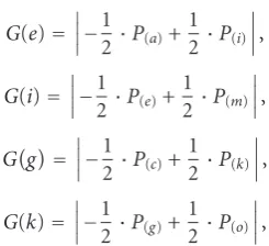
The intensity gradient filter for vertical orientation is applied to four pixels (e,i,g, andk) as shown inFigure 10(a) and calculated using the following equation.

G(e)=−1

2·P(a)+ 1 2·P(i)

,

G(i)=−1

2·P(e)+ 1 2·P(m)

,

Gg=−1

2·P(c)+ 1 2·P(k)

,

G(k)=−1

2·P(g)+ 1 2·P(o)

,

G(ver)=G(e) +G(i) +Gg+G(k)2.

(4)

Figure 10(b)is an intensity gradient filter orientation for four

pixels (b,c,j, andk) using(5)

G(b)=−1

2·P(a)+ 1 2·P(c)

,

G(c)=−1

2·P(b)+ 1 2·P(d)

,

Gj=−1

2·P(i)+ 1 2·P(k)

,

G(k)=−1

2·P(j)+ 1 2·P(l)

,

G(hor)=G(b) +G(c) +Gj+G(k)2, (5)

Edge_amplitude= |G(ver) +G(hor)|. (6)

The intensity diﬀerences in the vertical and horizontal directions are computed. Using these values, we determine the homogeneity of the block using an appropriate threshold value. By using all the above conditions, we then check the homogeneity of the block, which is explained in the following sub-sections.

3.3. Spatial Homogeneity. In order to decide whether a block is homogeneous, we use the sum of the edge amplitudes of the block, as shown in (7). If the block pixel amplitude is less than that of the predefined threshold, then the block is homogeneous; otherwise, it is non-homogeneous:

i,j∈A×A

Edge amplitude<Th. (7)

The above condition is the same for 8×8 block sizes except for the value of the pre-defined threshold. The threshold values for 16 × 16 and 8 ×8 block sizes are 295 and 8, respectively.

(9)

homogeneous; otherwise, it is non-homogeneous as shown in

Temp homogenity=

i,j∈N×N

_I

i,j−Ji·j, (8)

Temphomogenity<Th, (9)

whereI(i, j) andJ(i, j) denote the pixel intensities in the previous MB and the present MB, respectively. We adopt this common method since our main aim is to develop a pre-processing algorithm suitable for VLSI realization. Therefore, it helps to maintain a regular structure without increasing the complexity of the proposed algorithm. The above condition is applicable for 8×8 block sizes except for the threshold value. The threshold values are 420 and 115 for 16×16 and 8×8, respectively.

3.5. Overall Flow of the Classified Region Algorithm (CRA).

In order to maintain a regular structure in the proposed algorithm, the hierarchical order is maintained by choosing 16×16 block conditions first and 8×8 blocks later on (see

Figure 12).

In our classified region pre-processing algorithm, the homogeneous blocks not only choose 16× 16, but also 8

×16 or 16 ×8 block sizes. Therefore, block sizes 8 ×16 and 16× 8 are chosen according to the edge direction of the block. For example, as shown inFigure 11(a), if a block has a vertical edge we choose the 8×16 block size. If a block has a horizontal edge as shown inFigure 11(b), we choose the 16×8 block size. In order to detect the edge direction, we use the precomputed edge direction results from (4) and (5). We then compare the two results to decide the block size as follows:

G(ver)> G(hor)8×10,

G(ver)< G(hor)16×8.

(10)

Although we choose the rectangular block using edge direction, 16×16 is chosen for some blocks with edges. In order to avoid this situation, our algorithm always chooses 16 × 16 with 8 × 16 or 16 × 8 for RDO calculations. The performance of the proposed CRA algorithm is thus maintained. It should be noted that we do not increase the overhead to decide between 8×16 or 16 ×8 since we use the pre-computed edge direction values from CRA that are shown in (4) and (5). If a block is temporally homogeneous, we do not include intra mode for RDO calculations because intra mode is used to exploit spatial correlations. The mode decision procedure for 8×8 blocks is the same as that for 16

×16 MB.

3.6. Complexity Analysis. In this section, we analyze the complexity of the proposed method. Our method greatly reduces complexity, about 67%, compared to the conven-tional method. A convenconven-tional encoder employs the RDO method, which includes full mode search to choose the best block size. Therefore, only one block size and the associated motion vector (MV) can be chosen to encode a macroblock;

all other block sizes and associated MVs are discarded. Hence, a conventional JM increases the complexity whereas our proposed method reduces the number of inter modes without increasing the overhead of the inter mode decision. The proposed method avoids the exhaustive full mode search method, which includes all seven modes plus two intra modes for RDO calculation.

4. Experimental Results and Discussion

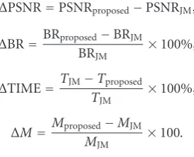
The proposed CRA fast mode decision algorithm was imple-mented on JM11.0, provided by JVT [24], with the following test conditions. In our simulation, the total number of frames was 200, the number of reference frames was one, RD optimization was enabled, main profile had sequence type IPPP, the search range was±16, and CAVLC was enabled. Tables1and2show the summary of performance, which is calculated according to the numerical averages with diﬀerent QP (24, 28, and 32) values. We defined four measures for evaluating the encoding performance, including average PSNR, average BR, average mode number saving factorM, and an encoding-time saving factorT, which are all defined as follows:

ΔPSNR=PSNRproposed−PSNRJM,

ΔBR=BRproposed−BRJM

BRJM ×

100%,

ΔTIME=TJM−Tproposed TJM ×

100%,

ΔM=Mproposed−MJM MJM ×

100.

(11)

If mode number saving factor (M) and time saving factor (Time) value increase, performance speed increases. It must be noted that positive values for the average PSNR and bit-rate indicate increments and negative values indicate decrements. Table 3 shows the average values of PSNR, bitrate, mode saving factor, and encoding time reduction. From the results, we can see that the proposed algorithm achieves a better mode number factor and encoding time reduction with a minimal loss of image quality and a minimal bit increment. Here, the mode number saving factor and encoding time reduction are higher than those of the existing methods [16,17]. The proposed algorithm reduces the complexity of the inter mode decision without increasing the complexity of the pre-processing stage with a negligible bit-rate increment, but provides a higher mode saving factor and encoding time reduction in most sequences. Our proposed method was compared with the recent work as shown inTable 4.

5. Conclusion

(10)

while maintaining negligible degradation in objective and subjective video quality. Therefore, this algorithm can be used as pre-processing unit for inter prediction units to decrease RDO complexity and encoding time.

Acknowledgment

This paper is supported in part by Korea University research grant.

References

[1] Draft ITU-T Recommendation and Final Draft Interna-tional Standard of Joint Video Specification (ITUT Rec. H.264/ISO/IEC 14496-10 AVC), March, 2003.

[2] T. Wiegand, G. J. Sullivan, G. Bjøntegaard, and A. Luthra, “Overview of the H.264/AVC video coding standard,”IEEE Transactions on Circuits and Systems for Video Technology, vol. 13, no. 7, pp. 560–576, 2003.

[3] G. Sullivan, T. Wiegand, and K.-P. Lim, “Joint model reference encoding methods and decoding concealment methods,” in Proceedings of the 9th Joint Video Term Meeting (JVT-I049d0), San Diego, Calif, USA, September 2003.

[4] E.-H. Yang and X. Yu, “Rate distortion optimization for H.264 interframe coding: a general framework and algorithms,”IEEE Transactions on Image Processing, vol. 16, no. 7, pp. 1774–1784, 2007.

[5] L. Yang, Y. Keman, J. Li, and S. Li, “An eﬀective variable block-size early termination algorithm for H.264 video coding,”IEEE Transactions on Circuits and Systems for Video Technology, vol. 15, no. 6, pp. 784–788, 2005.

[6] E. A. Al Qaralleh and T.-S. Chang, “Fast variable block size motion estimation by adaptive early termination,”IEEE Transactions on Circuits and Systems for Video Technology, vol. 16, no. 8, pp. 1021–1026, 2006.

[7] Z. Zhou and M.-T. Sun, “Fast macroblock inter mode decision and motion estimation for H.264/MPEG-4 AVC,” in Proceedings of the International Conference on Image Processing (ICIP ’04), pp. 243–263, October 2004.

[8] Y. H. Moon, G. Y. Kim, and J. H. Kim, “An improved early detection algorithm for all-zero blocks in H.264 video encoding,”IEEE Transactions on Circuits and Systems for Video Technology, vol. 15, no. 8, pp. 1053–1057, 2005.

[9] H. Wang, S. Kwong, and C.-W. Kok, “An eﬃcient mode decision algorithm for H.264/AVC encoding optimization,” IEEE Transactions on Multimedia, vol. 9, no. 4, pp. 882–888, 2007.

[10] B. Feng, G.-X. Zhu, and W.-Y. Liu, “Fast adaptive inter-prediction mode decision method for H.264 based on spatial correlation,” inProceedings of the IEEE International Sympo-sium on Circuits and Systems (ISCAS ’06), pp. 1804–1807, May 2006.

[11] C.-H. Kuo, M. Shen, and C.-C. J. Kuo, “Fast inter-prediction mode decision and motion search for H.264,” inProceddings of the IEEE International Conference on Multimedia and Expo (ICME ’04), vol. 1, pp. 663–666, June 2004.

[12] J. You, W. Kim, and J. Jeong, “16×16 macroblock partition size prediction for H.264 P slices,”IEEE Transactions on Consumer Electronics, vol. 52, no. 4, pp. 1377–1383, 2006.

[13] C. Grecos and M. Y. Yang, “Fast inter mode prediction for P slices in the H264 video coding standard,”IEEE Transactions on Broadcasting, vol. 51, no. 2, pp. 256–263, 2005.

[14] Y.-H. Kim, J.-W. Yoo, S.-W. Lee, J. Shin, J. Paik, and H.-K. Jung, “Adaptive mode decision for H.264 encoder,”Electronics Letters, vol. 40, no. 19, pp. 1172–1173, 2004.

[15] D. Wu, F. Pan, K. P. Lim et al., “Fast intermode decision in H.264/AVC video coding,”IEEE Transactions on Circuits and Systems for Video Technology, vol. 15, no. 7, pp. 953–958, 2005. [16] X. Jing and L.-P. Chau, “Fast approach for H.264 inter mode decision,”Electronics Letters, vol. 40, no. 17, pp. 1050–1052, 2004.

[17] I. Choi, J. Lee, and B. Jeon, “Fast coding mode selec-tion with rate-distorselec-tion optimizaselec-tion for MPEG-4 Part-10 AVC/H.264,” IEEE Transactions on Circuits and Systems for Video Technology, vol. 16, no. 12, pp. 1557–1561, 2006. [18] D. S. Turaga and T. Chen, “Classification based mode decisions

for video over networks,”IEEE Transactions on Multimedia, vol. 3, no. 1, pp. 41–52, 2001.

[19] L. Salgado and M. Nieto, “Sequence independent very fast mode decision algorithm on H.264/AVC baseline profile,” in Proceedings of the IEEE The International Conference on Image Processing (ICIP ’06), pp. 41–44, October 2006.

[20] S.-H. Ri, Y. Vatis, and J. Ostermann, “Fast inter-mode decision in an H.264/AVC encoder using mode and Lagrangian cost correlation,” IEEE Transactions on Circuits and Systems for Video Technology, vol. 19, no. 2, pp. 302–306, 2009.

[21] D. Liu, X. Sun, F. Wu, and Y.-Q. Zhang, “Edge-oriented uni-form intra prediction,”IEEE Transactions on Image Processing, vol. 17, no. 10, pp. 1827–1836, 2008.

[22] B. Girod, “Eﬃciency analysis of multihypothesis motion-compensated prediction for video coding,”IEEE Transactions on Image Processing, vol. 9, no. 2, pp. 173–183, 2000.

[23] X. Liu, D. L. L. Wang, and A. Srivastava, “Image segmentation using local spectral histograms,” inProceedings of the IEEE International Conference on Image Processing (ICIP ’01), pp. 70–73, October 2001.