DOI: 10.1534/genetics.107.080069
Gene Network Inference via Structural Equation Modeling in Genetical
Genomics Experiments
Bing Liu,*
,†,1,2Alberto de la Fuente
†,‡,1and Ina Hoeschele*
,†,3*Department of Statistics, Virginia Polytechnic Institute and State University, Blacksburg, Virginia 24061,†Virginia Bioinformatics Institute, Virginia Polytechnic Institute and State University, Blacksburg, Virginia 24061-0477 and‡CRS4 Bioinformatica,
Parco Scientifico e Tecnologico, POLARIS, 09010 Pula (CA), Italy
Manuscript received August 6, 2007 Accepted for publication January 7, 2008
ABSTRACT
Our goal is gene network inference in genetical genomics or systems genetics experiments. For species where sequence information is available, we first perform expression quantitative trait locus (eQTL) mapping by jointly utilizing cis-, cis–trans-, and trans-regulation. After using local structural models to identify regulator–target pairs for each eQTL, we construct an encompassing directed network (EDN) by assembling all retained regulator–target relationships. The EDN has nodes corresponding to expressed genes and eQTL and directed edges from eQTL tocis-regulated target genes, fromcis-regulated genes to
cis–trans-regulated target genes, fromtrans-regulator genes to target genes, and fromtrans-eQTL to target genes. For network inference within the strongly constrained search space defined by the EDN, we propose structural equation modeling (SEM), because it can model cyclic networks and the EDN indeed contains feedback relationships. On the basis of a factorization of the likelihood and the constrained search space, our SEM algorithm infers networks involving several hundred genes and eQTL. Structure inference is based on a penalized likelihood ratio and an adaptation of Occam’s window model selection. The SEM algorithm was evaluated using data simulated with nonlinear ordinary differential equations and known cyclic network topologies and was applied to a real yeast data set.
S
YSTEM biologists are interested in understanding how DNA, RNA, proteins, and metabolites work together as a complex functional network. Projecting this network onto the gene space (Brazhniket al.2002)yields a gene network, where only the relationships be-tween genes are modeled, although the physical in-teractions between genes are mediated through other components. While networks including genes, RNA, proteins, and metabolites would be more informative, gene networks are system-level descriptions of cellular physiology and provide an understanding of the ge-netic architecture of complex traits and diseases.
Bayesian networks are currently a popular tool for gene network inference (Friedman et al. 2000; Pe’er
et al.2001; Harteminket al.2002; Imotoet al.2002; Yoo
et al. 2002). Bayesian networks use partially directed graphical models to represent conditional indepen-dence relationships among variables of interest and are suitable for learning from noisy data (e.g., micro-array data) (Friedman et al.2000). Bayesian networks
are directed acyclic graphical (DAG) models, which
cannot represent structures with cyclic relationships. However, gene networks reconstructed on the basis of genetical genomics (or other perturbation) experi-ments are expected and have been found to be cyclic. Gene networks are phenomenological networks whose edges represent causal influences. These can be physical binding of a transcriptional regulator to the target promoter or more complicated biochemical mecha-nisms (involving signal transduction and metabolism), as there is much genetic regulation beyond transcrip-tion factors (Brazhniket al.2002). Recent articles point
to the need for methods that can infer cyclic networks, note the limitation of the Bayesian network approach (Lum et al. 2006), and show better performance of a
linear regression method over a Bayesian network al-gorithm most likely due to the presence of cycles (Faith
et al.2007). An alternative approach to the reconstruc-tion of directed cyclic networks (directed cyclic graphs, DCGs) is based on the assumption that a cyclic graph represents a dynamic system at equilibrium (Fisher
1970) and includes a time dimension to produce a causal graph without cycles (DAG), which then can be studied using Bayesian networks, an approach called dynamic Bayesian networks (Murphyand Mian 1999;
Hartemink et al. 2002). However, this approach
re-quires the collection of time series data, which is dif-ficult to accomplish, as it requires synchronization of
1These authors contributed equally to this work.
2Present address: Monsanto, 3302 SE Convenience Blvd., Ankeny, IA 50021.
3Corresponding author:Virginia Bioinformatics Institute, Virginia Poly-technic Institute and State University, Blacksburg, VA 24061-0477. E-mail: [email protected]
cells and close time intervals not allowing for feedback (Spirteset al.2000).
Xionget al.(2004) were the first to apply structural
equation modeling (SEM) to gene network reconstruc-tion using gene expression data. However, their ap-plication was limited to gene networks without cyclic relationships by using a recursive SEM, which has an acyclic structure and uncorrelated errors and is equiv-alent to a Gaussian Bayesian network. These authors re-constructed only small networks with,20 genes. Here, we apply SEM in the context of genetical genomics experiments.
In genetical genomics ( Jansenand Nap2001, 2004;
Jansen2003), a segregating population of hundreds of
individuals is expression profiled and genotyped. With expression quantitative trait locus (eQTL) mapping and selection of regulator–target pairs, an encompassing directed network (EDN) of causal regulatory relation-ships among gene expression levels (expression traits, ‘‘e-traits’’) and eQTL can be constructed. The network is called ‘‘encompassing’’ because it contains regulators with both direct and indirect effects on the same targets, which are actually only indirect regulations, and multi-ple candidate regulator genes for a given eQTL and target.
We present an SEM implementation to search for a set of sparser structures within the EDN that are well sup-ported by the data. The method is evaluated on simu-lated data with known underlying network structures and on a real yeast data set. Typically, SEM analyses have included at most tens of variables, but our implementa-tion is capable of reconstructing networks of several hundred genes and eQTL on the basis of a factorization of the likelihood and a strongly constrained network topology search space.
The genetic variation in a segregating population has been utilized to construct interaction networks among component traits or subphenotypes of complex dis-eases. Nadeauet al.(2002) reconstructed a network of
component traits of the cardiovascular system using phenotypic data on a segregating population and Bayes-ian network analysis, while Liet al. (2006) analyzed both
phenotypic and DNA marker data on a segregating population to construct networks including subpheno-types and QTL related to obesity and bone geometry, using SEM. While in this article we focus on using SEM to infer a gene regulatory network using e-traits only, it would not be too difficult to extend the method to the combined network inference including all of the above: genes, eQTL, disease (sub)phenotypes, and other phe-notypes such as metabolomic data.
METHODS
The methodology we discuss here can be applied to any organism where a segregating population is
exten-sively marker genotyped and expression profiled and where DNA sequence information is available. We perform gene (regulatory) network inference by a three-step approach: (1) eQTL mapping, (2) regulator– target pair identification to obtain the EDN, and (3) a search for a set of sparser optimal networks within the search space defined by the EDN. For the evaluation of this three-step approach, we analyzed the yeast genetical genomics data set (Brem and Kruglyak2005). After
removing the 20% of genes with the lowest e-trait var-iability from the original data, our data set contained e-traits for 4589 genes and genotypes for 2956 genetic markers on 112 haploid offspring from a cross between a laboratory and a wild strain (see supplemental mate-rial at http://www.genetics.org/supplemental/ for data preprocessing). We performed a small simulation study to evaluate the regulator–target pair selection. For eval-uation of the SEM in step 3, we developed a method to simulate genetical genomics data with known underly-ing network topologies, and we assessed the SEM on the basis of its ability to infer these networks.
Expression QTL analysis: We used three different eQTL mapping strategies, and we applied false discov-ery rate (FDR) control using the Benjamini–Hochberg procedure (Benjaminiand Hochberg1995). To
iden-tify chromosomal regions affecting multiple e-traits, the eQTL regions of two different e-traits were combined into a single region if the two eQTL were located at the same marker or their confidence intervals (C.I.’s) over-lapped by.80%. The first strategy wascis-eQTL map-ping, where only the marker(s) closest to the location of an e-trait’s gene are tested (e.g., Dosset al.2005), and
subsequently the secondary targets of thecis-eQTL, the so-calledcis–trans-regulated e-traits, are found by testing the effects of the identifiedcis-eQTL regions on other e-traits.
Multiple-trait analysis can provide more power to detect pleiotropic QTL. It is therefore desirable to utilize, in some way, the information from multiple correlated expression profiles in the search for eQTL. Therefore, we used two approaches that utilize infor-mation from correlated e-traits: QTL mapping of prin-cipal components (PC) andtrans-eQTL mapping. It has been shown that using a small number of PC traits for QTL mapping, when a (large) number of original traits are (highly) correlated (in groups of traits), is very effective for QTL identification;i.e., essentially the same QTL are identified by analyzing PC and original traits (Ma¨ hleret al.2002; see also Jiangand Zeng1995 and
Mangin et al. 1998). We used k-means with absolute
two genes. An eigenvalue cutoff of 1.5 was used to retain PCs within each cluster, so that the PCs from different clusters contained a similar amount of information. An eQTL affecting a PC was assumed to be a common regulator of all e-traits with high loadings, but there was no clear cutoff for ‘‘high.’’ Therefore, all e-traits were individually tested only for the identified PC–eQTL regions. Forcisand PC mapping, we performed single-marker analysis using the Kruskal–Wallis test (Lehmann
1975).
Trans-regulated e-traits are affected by an eQTL genotype and the e-trait of the corresponding candidate regulator gene simultaneously. Therefore, Kulp and
Jagalur(2006) proposed to include candidate
regula-tory e-traits in the QTL model. While these authors performed interval mapping, we used a regression model and the intersection-union test (IUT) (Casella
and Berger1990) to test whether the eQTL genotype
and the e-trait of the candidate regulator gener both significantly affect the e-trait of target genet
ytn¼b1yrn1b2xrn1b3yrnxrn1etn; n¼1;. . .;N; ð1Þ where ytn and yrn are deviations of e-trait values in
observationnfrom their means,xrnis the deviation of
the genotype value (0 or 1) from its mean for the marker closest to the physical location of candidate regulator gener, andetn is a residual. Coefficientsb1andb2(b3)
represent main effects (interaction) of gene and eQTL regulators, and both must be significantly different from zero for generto be declared as atrans-regulator of gene t as determined by the IUT. There are two reasons why thetrans-analysis might give false positives: the presence of a cis-eQTL affecting the target and multicollinearity betweenyrandxr. We therefore did not
consider any candidate regulator whose closest marker had a recombination rate of #0.25 with the marker closest to the target e-trait. We performed multicollinear-ity tests (see supplemental material), which indicated that our trans-mapping results should essentially be unaffected by multicollinearity.
Regulator–target pair identification and encompass-ing directed network: In contrast with previous work (e.g., Dosset al.2005; Kulpand Jagalur2006), in this
article we considercis-,cis–trans-, andtrans-regulations jointly with the goal of reconstructing an EDN that de-fines the network search space for network inference by SEM. While the SEM represents a global structural model evaluating regulator–target relationships in the context of an entire network, for regulator–target pair identification we use single equations (similar totrans -mapping) expressing the e-trait of a target gene as a linear combination of the expression levels of some of its regulator genes and eQTL. We therefore refer to these single equations as local structural models or equations. Regulator–target pair identification for cis and PC map-ping: For the eQTL identified bycis-and PC mapping,
the regulator–target pair selection was performed in three steps separately for each eQTL: (1) identification of those of the detectedcis-linked e-traits that were most likely trulycis-linked and those that were probablycis– trans-effects, (2) identification of those of the detected trans-affected e-traits that were probablycis–trans-affected rather than likelytrans-affected, and (3) a search for the candidate regulator among all genes physically located in the eQTL C.I. for each of the likelytrans-affected e-traits. 1. Distinguishingcisfromcis–trans: We tested whether a cis-affected gene t was likely truly cis-affected using model (1) but omitting the interaction term, withr denoting any other gene found to becis-affected by the same eQTL and withxrndenotingthe genotype of
the marker at which the peak test statistic of the eQTL occurred. Ifytis actuallycis–trans-affected throughyr,
then b2 should not be significantly different from zero withyrincluded in the regression equation. If for
an e-traitt,b2remained significant (at theP ,0.05 level) for all e-traitsr, then it was identified as a ‘‘true’’ cis-affected e-trait.
2. Distinguishingtransfromcis–trans: Using model (1) again,ytis now atrans-affected e-trait, andyris acis
-affected e-trait identified in step 1.Cis–trans regula-tion is indicated byb2not being significantly different from zero. Ifb2remains significant for allcis-affected e-traitsr, then gene t is identified as a likely trans -affected e-trait.
3. Selecting regulator–target pairs in the same eQTL region: To find the candidate regulator(s) for a likely trans-affected e-trait t among all genes physically located in the eQTL region, for target e-trait t we fitted model (1) with any candidate regulator e-traitr located in the eQTL region and the eQTL marker (without the interaction term) and any additional candidate regulator e-traitr9. The additional candi-date e-trait was included to examine whether the regulator–target correlation was due to some indirect mechanism. We retained the maximum P-value of theb1coefficients foryracross allr9and if it was
sig-nificant, then we retained the regulator–target pair (r, t)½we used a P-value cutoff of (0.05/number of candidate regulators) for all tests performed for each eQTL–target pair.
Identification of regulator–target pairs for trans-mapping: For each target e-trait t with at least two identified regulators, for each identified regulatorrof e-traitt, we included another identified regulator e-trait (r9) of t and its nearest marker in model (1) to obtain
ytn¼ ðb1ryrn1b2rxrn1b3ryrnxrnÞ
1ðb1r9yr9n1b2r9xr9n1b3r9yr9nxr9nÞ1etn: ð2Þ
for regulator r was,0.25. We retained the maximum P-value of the IUT test forb1randb2racross allr9and if
it was significant (at theP,0.05 level), only then we re-tained the regulator–target pair (r,t). Otherwise we dis-carded generas a regulator of tand assumed that its effect was due to an indirect mechanism.
Simulation study on regulator–target pair identification: We evaluated our regulator–target pair selection in a small simulation study. For a population of 112 individ-uals (as in the yeast data), we simulated an eQTL region containing three eQTL causal polymorphisms and several candidate regulator and target genes. This local network is depicted in Figure 1, with G (Q) representing a gene (eQTL). The target list for the eQTL region is T¼ ½G2, G3, G4, G5, G6, G7, G8. Gene G1 is the only candidatetrans-regulator, while genes G3, G4, G6, and G7 are candidatecis-regulators. There are four types of regulations: one truetrans-regulation (from G1 and Q1 to G2), two truecis-regulations (Q2 to G3 and Q3 to G6), two true cis–trans-regulations of targets located in the eQTL region (Q2 to G3 to G4 and Q3 to G6 to G7), and two truecis–trans-regulations of targets not located in the eQTL region (Q2 to G3 to G5 and Q3 to G6 to G8).
Data were simulated with linear regression models with regression coefficients fixed at the value of 1 and residual standard deviations (SD) set to 0.125, 0.25, or 0.5 (one value for all genes, or for genes with odd numbers SD ¼ 0.5 or 0.25, and for genes with even numbers SD¼0.25 or 0.125). For a gene directly reg-ulated by an eQTL, the model wasy¼bx1e¼x1e, where x is QTL genotype (0/1), variance due to the eQTL was 0.25, and heritability was 0.25/(0.251SD2)¼ 0.941, 0.80, or 0.50 for the three SD values, respectively. For a gene indirectly regulated by an eQTL (Q2/G3 /G4), the model wasy2¼b(bx1e1)1e2¼x1e11e2, and heritability was 0.25/(0.2512 SD2)¼0.889, 0.667, and 0.333. The three causal polymorphisms in the eQTL region had order Q1–Q2–Q3 (see Figure 1) with recombination rater¼0.0 orr¼0.09 between adjacent polymorphisms. A total of 1000 data replicates were simulated and analyzed for each of several combina-tions of SD andrvalues.
EDN construction:The eQTL mapping and regulator– target pair selection steps resulted in three lists of causal regulatory relationships: (1) a list containing all identi-fiedcis-regulations (eQTL A affects gene A located in its confidence region), (2) a list containing all cis–trans -regulations (cis-regulated gene A regulating gene B), and (3) a list containing alltrans-regulations ½gene A regulating gene B and eQTL A affecting gene B (but not gene A). To construct an EDN, we assembled all the identified and retained regulator–target relationships, which consisted of directed edges (representing causal influences) from eQTL to cis-regulated target genes, from cis-regulated genes to cis–trans-regulated target genes, fromtrans-regulator genes to target genes, and
fromtrans-eQTL to target genes. The EDN consisted of two types of nodes: continuous nodes for the genes (e-traits) and discrete nodes for the eQTL (genotypes).
Structural equation modeling: A structural equation model: SEM has been widely used in econometrics, so-ciology, and psychology, usually as a confirmatory pro-cedure instead of an exploratory analysis for causal inference (e.g., Johnston1972; Judgeet al.1985; Bollen
1989). Shipley(2002) discusses the use of SEM in biology
with an emphasis on causal inference. SEM has been used for association and linkage mapping of QTL (e.g., Neale
2000; Steinet al. 2003). In contrast, we treat the eQTL
as known in the SEM, as the high-dimensional nature of the e-traits forces us to perform a three-step analysis (eQTL mapping, EDN construction, and SEM network sparsification).
In general, an SEM consists of a structural model describing (causal) relationships among latent variables and a measurement model describing the relationships between the observed measurements and the underly-ing latent variables. Any SEM can be represented both algebraically through a system of equations and graph-ically. A special case is the SEM with observed variables only, where all variables in the structural model are observed, and therefore there is no measurement model. Our model is a SEM with observed variables, which can be represented as
yi ¼Byi1Fxi1ei; ei ð0;EÞ i¼1;. . . ;N: ð3Þ In this model, for samplei(i¼1,. . .,N),yi¼(yi1,. . ., yip)Tis the vector of expression values of all (p) genes in
the network, andxi¼(xi1,. . .,xiq)Tdenotes the vector of
marker or eQTL genotype codes. Theyiand thexiare deviations from means,eiis a vector of error terms, and
Eis its covariance matrix.
Matrix B contains coefficients for the direct causal effects of the genes on each other: Element bkm
rep-resents the effect of e-trait m on e-trait k. Matrix F
contains coefficients for the direct causal effects of the eQTL on the genes: Elementfkmrepresents the effect of
eQTLmon e-traitk. The structure of matricesBandF
corresponds to the path diagram or directed graph representing the structural model, in which vertices or nodes represent genes and eQTL and edges correspond to the nonzero elements inBandF. MatricesBandFare sparse when the model represents a sparse network. When the elements ineiare uncorrelated and matrixB
can be rearranged as a lower triangular matrix, the model is recursive, there are no cyclic relationships, and the graph is a DAG. If the error terms are correlated (Eis nondiagonal), or matrixBcannot be rearranged into a triangular matrix (indicating the presence of cycles), the model is nonrecursive. The graph corresponding to a nontriangular matrixBis a DCG.
are sampled from a segregating population. However, the joint likelihood of the yi and xi can be factored into the conditional likelihood of the yi given the xi
times the likelihood of the xi, and the latter does not depend on any of the network parameters in B,
F, andEand can therefore be ignored. Thus, we need only to assume multivariate normality for the residual vectors.
An important issue in nonrecursive SEM or DCG is equivalence. Models are equivalent when they cannot be distinguished in terms of overall fit. For DAGs, al-gorithms for checking the equivalence of two models or for finding the equivalence class of a given model in polynomial time are available (Vermaand Pearl1991;
Anderssonet al.1997). Therefore, model search is
per-formed among equivalence classes rather than among individual DAGs (Chickering2002a). An equivalence
class discovery algorithm for DCGs, which is polynomial time on sparse graphs (Richardson1996; Richardson
and Spirtes1999), is available but there is no algorithm
for model search among equivalence classes. Two DAG models are equivalent if they have the same undirected edges but differ in the direction of some edges (edge reversal) (Pearl2000). Two DCG models can be
equiv-alent even if they differ in their undirected edges (Richardson1996; Richardsonand Spirtes1999). In
our case, two models cannot be equivalent under edge reversal, because the directions of the edges are de-termined by the eQTL. By using an information crite-rion for model selection with a penalty for the number of parameters, we prefer the sparser model of two equivalent models that differ in the number of edges. Therefore, equivalence is of less concern in our case. Instead of selection among equivalence classes, we use a model search algorithm that selects multiple models (described below).
A main concern about using SEM for gene net-work inference is the severe constraint on the netnet-work size when using existing SEM software ½e.g., LISREL ( Jo¨ reskog and So¨ rbom 1989) and Mx (Neale et al.
2003). Typical applications of SEM include models with at most tens of variables. No existing software program can analyze models with a size relevant to genomics (hundreds or even thousands of variables). Even the SEM implementation of Xionget al.(2004), which employed a
genetic algorithm, was applied only to small networks of
,20 genes. Here, we implement SEM analysis in the con-text of genetical genomics experiments, where the EDN provides a strongly constrained topology search space, allowing us to reconstruct networks with up to several hundred genes and eQTL.
Algorithms for likelihood maximization: The most com-monly used estimation method for SEM is the maxi-mum-likelihood (ML) method. Assuming a multivariate normal distribution of the residual vectors, oreiN(0,
E), the logarithm of the conditional likelihood of theyi’s
given thexi’s and given a particular structure is
Lðy1;. . .;yNjB;F;E;x1;. . .;xNÞ
¼constant1N lnðjIBjÞ1N
2lnðjEj
1Þ
1
2
XN
i¼1
ððIBÞyiFxiÞ9E1ððIBÞyiFxiÞ: ð4Þ
This log likelihood is maximized with respect to the parameters inB,F, andE.
A nonrecursive SEM model can be underidentified, while a recursive SEM is always identified. A model is ‘‘identified’’ if all parameters are independent functions of the data covariance matrix. Under regularity assump-tions, an underidentified model can be equivalent to an identified model nested within it (Bekkeret al.1994).
Since we prefer the sparser model, our model selection based on an information criterion should arrive at identified models (an SEM can be checked numerically for underidentification by computing the rank of the information matrix or by repeated model fitting).
The likelihood function is nonlinear in the parame-ters, and therefore an iterative optimization procedure is required for its maximization. The likelihood can be factored into a product of local likelihoods that all depend on different sets of parameters and that are maximized individually in analogy with Bayesian net-work analysis. For directed acyclic graphs, the global directed Markov property permits the joint probability distribution of the variables to be factored according to the DAG (Pearl2000). LetVbe the random variable
associated with a particular node (vertex). The factor-ization can be represented as p(V1,V2,. . .,Vn)¼Pnj¼1 p (Vj j V(parents of j), uj), whereV(parents of j) is a
vector ofV’s of the parent vertices of vertexj, andujis the
parameter vector of the local likelihood p(Vj j .). A
network with cyclic components (systems of connected cycles, in which any gene can find a path back to itself through any other genes) becomes acyclic when a set of genes pertaining to the same cyclic component is collapsed into a single node; i.e., Vj represents either
an individual gene or the set of genes involved in the same cyclic component. If the error terms are also uncorrelated (diagonalE), thenp(V1,V2,. . .,Vn) can be
nodes, not eQTL nodes, with the latter appearing as parents of genes only in a cyclic component.
For a cyclic component c,p(VcjV(parents ofc),uc)
involves the equations for all genes in cyclic component cfrom (4),
yicc¼Bcyic1Fcxic1eic; eic ð0;EcÞ i¼1;. . .;N;
ð5Þ
whereyicis a vector of expression values in sampleifor all genes in cyclic componentcand their parent genes, which can be partitioned into subvectors yicc and yicp
pertaining to the genes in cyclic componentc and to their parent genes not in cyclic component c, respec-tively;Bc(Fc) is a submatrix obtained from the original
B(F) matrix by extracting all rows corresponding to the genes incand all columns pertaining to these genes and their parents; xic contains the genotype codes of all
eQTL parents of genes inc; andeicis the residual vector for all genes inc. MatrixBc can be further partitioned intoBcc andBcp, corresponding to columns pertaining to genes in c and parent genes not in c, respectively. Then
ðIBccÞyicc¼Bcpyicp1Fcxic1eic;
eic ð0;EcÞ i¼1;. . .;N; ð6Þ whereyicp is a vector of exogenous variables (variables that do not receive any inputs) just likexic. The likeli-hood function for this model is then
Lðyiccjyicp;Bcc;Bcp;Fc;Ec;xicÞ
¼constant1NlnðjIBccjÞ1 N
2lnð jEcj
1Þ
1
2
XN
i¼1
ððIBccÞyiccBcpyicpFcxicÞ9Ec1
3ððIBccÞyiccBcpyicpFcxicÞ: ð7Þ
The likelihood function (7) of the genes in a cyclic component is maximized using a genetic algorithm (GA)-based global optimization procedure. During the model search, the local likelihood of cyclecneeds to be remaximized with respect touconly if the set of parents
of genes involved in the cyclic component has changed. GA is a stochastic iterative optimization tool (Holland
1975, 1992; Goldberg1989). Although GA is
computa-tionally more expensive than the gradient-based meth-ods, it has been shown that GA is more successful for problems with very complex parameter spaces (Mendes
2001; Moles et al.2003). The GA C11 library GAlib
(http://lancet.mit.edu/ga/) was used in our implemen-tation. GA evaluates the fit of a chromosome using the objective function, which in our case is the log-likelihood function for genes in a cyclic component. With a
diag-onalEmatrix, the most computationally demanding part for evaluating the objective functions is the computation of the determinants of matrices (IB)c. These matrices
are sparse, and determinants are calculated using sparse LU decomposition as implemented in the C library UMFPACK, which applies the unsymmetric multifrontal method for sparse LU factorization (Davis and Duff
1997, 1999; Davis 2004a,b). Since the patterns of the
matrices remain the same for a given structure, symbolic factorization is performed only once, and the result is used by all numerical factorizations for objective func-tions of that structure.
In our model search algorithm, for remaximization of the local likelihood of a cyclic component, we use four types of starting values simultaneously in the initial GA population: random starting points, starting values obtained from two-stage least squares (2SLS) (described below), starting values equal to the current parameter estimates, and starting values from the current param-eter values for all genes except 2SLS estimates for the genes directly affected by the deletion or addition of an edge. We use current parameter values as starting values because we search the model space by removing and adding single or a few edges at a time, and therefore most parameter estimates do not change or do not change much. However, the parameter values associ-ated with the gene directly affected by the deletion or addition of an edge can change considerably and we hence initiated them by 2SLS. Using these starting values greatly increased the efficiency of the GA optimization.
2SLS (e.g, Judgeet al.1985; Goldberger1991) is a
computationally efficient parameter estimation method for SEM. The 2SLS estimates are computed on the basis of one portion of the model at a time, while ML esti-mation takes the entire model into account. Therefore, ML is called a ‘‘full information’’ method, while 2SLS is a ‘‘partial information’’ method, and ML estimates are generally better than 2SLS estimates. However, 2SLS is a noniterative approach and computationally very effi-cient. In 2SLS, the first step is to obtain predicted values ofyusing all of the exogenous variables in the system on the basis of the following reduced-form equations and their ordinary least-squares (OLS) fits,
yg¼Xpg1vg; g¼1;. . .;G
ˆyg¼X ˆpg ¼XðXTXÞ1XTyg; ð8Þ
where
yg¼
yg1 . . . ygN
2 4
3
5; XN3Q ¼
xT1
. . .
xTN 2 4
3
5;
PQ3G ¼ ½p1 . . .pG; P¼FTðIBTÞ1;
whereNis sample size,Gis the number of endogenous variables, andQis the number of exogenous variables in
X. The reduced-form equations are derived from (3) (details are given in our supplemental material). Pre-dictionsˆygare then used in the original model to obtain OLS estimates of the nonzero elements in each row ofB
(bg) and each row ofF(fg), or
yg ¼Ybˆ g1Xfg1eg¼Yˆ*b*g1X*f*g1eg
ˆ b*g
ˆf* g
2 4
3
5¼ X
*TX* X*TYˆ*
ˆ
Y*TX* Yˆ*TYˆ*
" #1 X*Ty
g
ˆ Y*Tyg
" #
; ð9Þ
where
Y¼ ½y1 . . .yG; X¼ ½x1 . . .xG; E¼ ½e1 . . .eG;
bg* andfg* are obtained frombg andfg by deleting all elements fixed at zero (in a given network structure), andY* andX* have the corresponding columns deleted fromYandX. 2SLS may not work well for some genes with no suitable instrumental variables. An instrumental variable for prediction of an endogenous variable exists only under certain conditions in cyclic networks (e.g., Heise1975). These conditions are likely not met for all
genes in a network. Only if each gene had acis-linked eQTL, would the conditions then always be met.
Network topology search:Alternative models or struc-tures (topologies) were compared using information criteria. Information criteria (IC) combine the maximized likelihood with a penalty term to adjust for the number of free parameters, and some also adjust for sample size. The information criteria we used include the Bayesian information criterion (BIC) (Schwartz1978) and a
modi-fication, BIC(d) (Bromanand Speed2002).
The EDN contains 2d
submodels, where d is the number of edges. It is impossible to exhaustively search this space even for EDNs of moderate size. Therefore, we adapted a heuristic search strategy based on the prin-ciple of Occam’s window model selection (Madigan
and Raftery1994) that potentially selects multiple
ac-ceptable models. Let A denote a set of acceptable models;C, the set of candidate models; andK, the set of models with minimum IC (the model selection cri-terion). The search algorithm includes a down and an up component. The down algorithm consists of the fol-lowing steps:
0. Initialize A and K as empty sets and C as a set containing only the EDN.
1. Select a modelM1inCand move it toA. Set ICmin¼0. 2. Select a submodel M2of M1by removing an edge fromM1and compute the model selection criterion for these two models, IC12.
3.
a. If IC12,T(i.e., modelM2is strongly better than M1), then removeM1fromAifM12A, addM2
toCifM2;C, setKto the empty set, and set ICmin¼ ‘.
b. Else if T , IC12 , ICmin(i.e., M2 is the best among all submodels ofM1considered so far), then set ICmin¼IC12, replace the model in setK withM2, and removeM1fromAifM12A. c. Else if ICmin , IC12 , 0 (i.e., model M2
im-provesM1but is not strongly better and is not the best among all submodels of M1 consid-ered so far), then (i) with probability w (e.g., w ¼ 0.20 or 0.10) this model is chosen as a candidate model by removing M1 from A if M12Aand adding M2toCifM2;C, or (ii) otherwise take no action.
d. Else take no action. 4.
a. If there are more submodels ofM1, then go to step 2.
b. Else move the model inKtoCif it is not already inC.
5. IfCis not empty, go to step 1.
Starting from all models accepted in the down algorithm, the up algorithm follows the same steps as in the down algorithm, except each time an edge that was removed from the EDN is added back into the model. Once the up algorithm is completed, the set A
contains the set of potentially acceptable models. For large networks with many removable edges, the original Occam’s window model-selection (Madigan
and Raftery 1994) approach may search a very large
model space. In the worst case, it is equivalent to an exhaustive search. Therefore, we imposed a threshold Ton the IC (step 3a). Only if the IC of the submodel strongly improves over the model it is nested in (IC,
T), is the sub-model then kept as a candidate model. Otherwise, if no submodel passesTand the minimum IC is less than zero, then the model with minimum IC is kept as a candidate model. The size of the search space depends on the value ofT. IfT¼ ‘and probabilitywis zero, the algorithm is similar to the greedy hill search
(Chickering 2002a,b). If ‘ , T , 0, then the
algorithm searches a larger network space and possibly accepts multiple models. Because T requires the sub-model to strongly improve over the sub-model it is nested in, it is likely that the search will accept only one final model. Therefore, probabilitywin step 3ci can be set to a positive value to introduce multiple search paths to be followed.
gene by an eQTL cannot be removed unless the eQTL has multiplecis-candidates, in which case one of thecis -edges needs to remain.
Data simulation for evaluation of SEM and network topology search: To evaluate the performance of the linear SEM for gene network inference, we simulated data with nonlinear kinetic functions and cyclic network topology in the context of a genetical genomics exper-iment with 300 recombinant inbred lines. We simulated QTL genotypes using the QTL cartographer software (Basten et al.1996) and steady-state (equal synthesis
and degradation rates and constant gene expression levels in time) gene expression profiles according to the simulated genotypes with the Gepasi software (Mendes
1993, 1997; Mendeset al.2003), using nonlinear
ordi-nary differential equations
dGi dt ¼Vi3
Y
j
Zj KIj Ij1KIj
!!
3Y
k
Zk 11 Ak Ak1KAk
kiGi1uiGi;
ð10Þ
whereGiis the mRNA concentration of genei,Viis its
basal transcription rate,KIj andKAk are inhibition and
activation rate constants, respectively,Ijand Akare
in-hibitor and activator concentrations, respectively (the expression levels of genes in the network affecting the expression of gene i), and ki is a degradation rate
constant. Each gene has two genotypes, and the poly-morphism is located either in its promoter region affecting its transcription rate (cis-linkage with V ¼1 for one genotype andV¼0.75 for the other) or in the coding region of a regulatory gene changing the basal transcription rates of the target genes by multiplyingV by a factorZ(Z¼1 for one genotype andZ¼0.75 for the other). Each gene has a 50% probability of having a promoter (cis-) or coding region (trans-) polymorphism. The error parameteruirepresents ‘‘biological’’ variance
and was sampled from a normal distribution with a mean 0 and a standard deviation of 0.1 each time before the calculation of a steady state. All other parameters were set to 1. Finally, we also added ‘‘experimental noise’’ to the generated data at 10% proportional to the variance of each gene’s expression values.
The parameters were chosen so that the estimated heritabilities were close to those found in real data. For a simulated data set, we calculated the heritability of an e-trait by dividing the steady-state variances simulated without biological and technical noise by the variance simulated with biological and technical errors. The simulated e-traits had an average heritability of 56% with 60% of the e-traits having heritabilities.57%. The simulated e-traits had somewhat lower heritabilities than the actual e-traits in the yeast data set where 60%
of the genes had estimated heritabilities.69% (Brem
and Kruglyak2005), which were calculated as (e-trait
variance in the segregants pooled e-trait variance among parental measurements)/e-trait variance in the segregants.
Random network topologies were generated as de-scribed by Mendes et al. (2003). For each generated
network we created an EDN by adding links from any nodeito nodej, if nodejwas no more than two edges separated from nodeiin the true network.
RESULTS
The regulator–target pair identification and the SEM method were tested on simulated data, and the entire three-step analysis was applied to the real data set from a yeast segregating population (Brem and Kruglyak
2005).
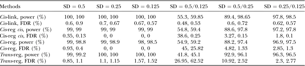
Simulation results on regulator–target pair identifi-cation: The results of our regulator–target pair identi-fication from simulated data for the single eQTL network in Figure 1 are summarized in Table 1 in terms of power and FDR (see Table 1 for definition of power and FDR) for four types of simulated regulatory effects (see Figure 1 and methods), which demonstrate that
the procedure works well, with the exception of a case where some genes have extremely high and other genes low heritability (column 5 in Table 1). This problem was actually due to one of thecis-linked genes (G3) having very small residual variance and being assigned as a reg-ulator for other genes incorrectly.
SEM analysis of simulated data:Ten data sets of 300 observations each, with different random network to-pologies, were analyzed. These networks had 100 genes, 100 eQTL, and on average 148 gene/gene and 123 Figure 1.—The network model used in the simulation
eQTL/gene edges. Their EDN contained on average 360 gene/gene and 301 eQTL / gene edges. On average 42 genes were involved in one to three cyclic components in each data set, with the biggest cyclic component involving on average 37 genes. The algo-rithm was run on a multiprocessor SGI Origin2000 and took between 2 and 8 hr (total time) per data set with an average of 4 hr. We report the results in terms of FDR and power. The FDR is expressed as the number of wrongly identified edges divided by the total number of identified edges. Power is defined as the number of edges correctly inferred as a fraction of the total number of edges in the true network. In Table 2, we compared results obtained using BIC and BIC(d). The results showed that for the simulated data sets, BIC was not sufficiently stringent for the eQTL/gene edges, with an average power of 99% and an average FDR of 22%. For the gene/gene edges, the average FDR was 8%, with average power of 88%. For the eQTL / gene edges, the average FDR with BIC(d) was 9%, while the
average power was 99%. For the gene /gene edges, with BIC(d) the average FDR was only 1%, while the power was reduced to on average 78%. Overall, the algorithm performed well, and the results show that the linear SEM appears to be robust under violation of the linearity assumptions.
While the above results were based on retaining a single, final SEM model, for some of the 10 data sets we allowed the topology search algorithm to follow 20 different, random search paths. This was done to de-termine whether there were different models (topolo-gies) with the same likelihood (equivalent models) and to identify multiple models with the same or nearly the same BIC ½or BIC(d). These additional networks con-tain important information that would be missed when searching only for a single network, and they reflect the uncertainty about the true network structure after observing the data. On average 16 very similar final models were obtained per data set. Of an average of 134 detected eQTL/gene edges, the average number TABLE 1
Results from a simulation study on regulator–target pair identification in a single-eQTL region with three causal polymorphisms and with multiple candidate regulator and target genes (true network structure is in Figure 1)
Methods SD¼0.5 SD¼0.25 SD¼0.125 SD¼0.5/0.125 SD¼0.5/0.25 SD¼0.25/0.125
Cis-link, power (%) 100, 100 100, 100 100, 100 55.3, 59.85 89.4, 98.65 97.8, 98.5
Cis-link, FDR (%) 0.6, 0.9 0.7, 0.67 0.67, 0.57 0.48, 0.53 0.6, 0.72 0.62, 0.57
Cis-regcis, power (%) 99, 99 99, 99 99, 99 54.8, 59.4 88.6, 97.8 97.2, 97.8 Cis-regcis, FDR (%) 0.35, 0.13 0, 0 0, 0 38.6, 0.25 3.27, 0.15 1.8, 0.1
Cis-reg, power (%) 99, 98.8 99, 98.9 98, 98.5 54.9, 59.2 88.2, 97.4 96.9, 97.5
Cis-reg, FDR (%) 0.93, 0.4 0, 0 0, 0 45, 25.82 4.82, 1.33 2.85, 1.3
Trans-reg, power (%) 99, 99.2 100, 100 100, 100 41.8, 45.1 92.9, 96.1 96.3, 96.5
Trans-reg, FDR (%) 0.85, 1.1 1.1, 1.15 1.57, 1.52 26.95, 62.52 10.92, 2.52 2.3, 2.77
Power, percentage of replicate data sets in which the regulation type was found; FDR, percentage of replicate data sets in which a regulation of a certain type was found that did not exist in the underlying network;Cis-link,cis-regulation of target in eQTL region;
Cis-reg,cis–trans-regulation of target not in eQTL region;Cis-regcis,cis–trans-regulation of target in eQTL region;Trans-reg,trans -regulation. For the last three columns, even-numbered gene nodes (Figure 1) received the left amount of error variance and odd-numbered nodes the right amount. The two numbers in each cell correspond to 0% recombination and 9% recombination among the three causal polymorphisms in the single-eQTL region, respectively. AP-value cutoff of 0.01 was used.
TABLE 2
Results of the SEM analysis on the simulated data
Edge type
Model
IC Measure 1 2 3 4 5 6 7 8 9 10
BIC F FDR 18.4 24.3 27.4 17.9 19.5 21.6 20.7 19.0 23.9 22.2
Power 100.0 100.0 100.0 100.0 100.0 99.2 99.2 100.0 97.5 100.0 B FDR 6.6 7.1 7.6 7.6 5.7 8.5 3.8 15.3 9.5 11.0
Power 87.6 89.7 89.9 89.3 89.3 88.4 85.9 85.8 88.7 87.2
BIC(d) F FDR 7.5 7.9 7.7 5.1 8.1 7.1 6.3 14.8 11.9 14.5
Power 100.0 100.0 99.2 99.2 100.0 96.7 100.0 98.4 100.0 100.0
B FDR 0.8 0.0 1.7 0.0 1.6 3.4 0.0 3.4 1.8 0.9
Power 80.7 82.2 79.9 78.5 81.2 76.2 77.9 77.7 72.7 71.8
of edges different from the best model was 4.4. Of an average of 153 detected gene/gene edges, the average number of edges different from the best model was 7.9. The average BIC difference to the best model was 26. The average likelihood difference was 12, while the mean likelihood was 26,969. Two models had the exact same likelihood (and hence were equivalent), while having six different eQTL / gene edges and seven different gene/ gene edges. Another four pairs of models had likelihood differences,1, with on average four different eQTL /gene edges and 7.3 different gene/gene edges.
Yeast data analysis: eQTL mapping: When analyzing PCs computed from separate PC analysis of the 100 gene clusters, a total of 250 combined eQTL regions (median size 37 kb) were identified. When testing these 250 eQTL on all individual e-traits, a total of 10,316 eQTL– target pairs were detected. Forcis-mapping, a total of 578 combined cis–eQTL regions (median size 36 kb) were identified. We then searched forcis–trans-affected e-traits and found a total of 7481 eQTL–target pairs.
Trans-mapping appeared to greatly increase the power to detect eQTL. A total of 41,309 significant candidate regulator–target pairs were identified. The interaction between eQTL and candidate regulator (b3in Equation 1) gene did not appear to be important. Of all tests performed, only 0.08% had a significant eQTL-by-regulator gene interaction with FDR control at the 5% level for this term. Of the tests with a significant IUT, 4.94% hadP-values forb3,0.01, and 0.43% had P-values smaller than the FDR cutoff from all tests. More details on the eQTL analysis and results can be found in our supplemental material.
Regulator–target pair identification and EDN construc-tion:For the 10,316 eQTL-target pairs identified by PC mapping, 9843 regulator-target pairs were retained, involving 3581 genes, with 1103 regulators and 3262 targets. For the 7481 eQTL–target pairs identified bycis -mapping, 6090 regulator–target pairs involving 3034 genes were found, with 1099 regulators and 2562 tar-gets. After local sparsification of thetrans-mapping re-sults, the 41,309 candidate regulator–target pairs were reduced to 15,835 pairs involving 3858 genes with 1433 regulators and 3682 targets. We combined these results into an EDN, which included 28,609 regulator–target pairs. This EDN can be found online in several file formats at http://www.bioinformatica.crs4.org/Members/ alf/genetics/.
The network consisted of 4274 gene nodes. The re-maining 315 genes did not receive any inputs nor were they affecting any other genes. A total of 2118 genes were regulators of at least one target, among which 158 did not receive any inputs. A total of 4116 genes were targets having at least one regulator, among which 2156 did not affect any other genes in the network. A total of 1960 genes occurred both as regulators and as targets. There were 135 instances of reciprocal regulation
pre-sent (gene A directly affects gene B and vice versa). Gene PHM7 had the most targets, 468; gene YLR152C had the most regulators, 32.
The confirmed regulators and the strong candidate regulator genes for the 13 eQTL with widespread tran-scriptional effects identified in Yvertet al. (2003) were
investigated in this EDN. Amn1, a confirmed regulator gene with widespread influence, was found to be a top cis–trans-regulator with 408cis–trans-targets. The strong candidate regulator MAK5 with five coding region polymorphisms between the two parental strains had 110 trans-targets. Another confirmed regulator gene GPA1 had 60 targets, about half of which are trans -targets. The genes LEU2 and URA3 had 98 (most were cis–trans) and 32 (most were cis–trans) targets, respec-tively. The heme-dependent transcription factor HAP1 had 141 targets (100cis–trans, the otherstrans).
SEM analysis: We performed SEM analysis on a sub-network of the EDN, which was obtained by starting out with 168 genes involved in a cycle and including all genes connected to the cycle genes by up to 3 edges and all the eQTL associated with these genes. The sub-EDN had 265 genes, 241 QTL, 832 gene/gene edges, and 640 eQTL/gene edges. After sparsification using our SEM implementation, the resulting network contained 475 gene/gene edges and 468 eQTL/gene edges. The SEM analysis took110 hr or 4.5 days (total time) on the multiprocessor SGI Origin2000. The network topology is available in our supplemental material, and the yeast subnetwork can be found online in several file formats at http://www.bioinformatica.crs4.org/Members/ alf/genetics/.
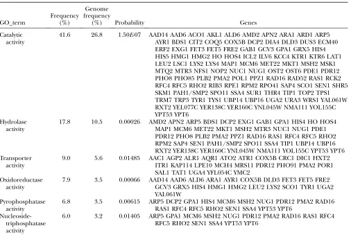
Table 3 shows the significant biological function groups of the genes in this network. About 41.6% of these genes are involved in catalytic activity, and another 18% are involved in hydrolase activity. All biological functions in Table 3 are significantly enriched in this network.
DISCUSSION
Our EDN construction and network inference meth-odology requires the availability of DNA sequence information and it explicitly considers cis-, cis–trans-, andtrans-regulation. This approach is most powerful, but it is possible to construct a causal gene network from a genetical genomics data set even in the absence of sequence data, although such an approach should have (much) reduced power. It is of course possible to map eQTL without specifically considering the different forms of regulation, and the power of such an approach can potentially be increased by including e-trait cova-riates as suggested by Perez-Encisoet al. (2007).
More-over, eQTL mapping permits (some degree of) causal inference even without knowing the candidate regula-tor genes in an eQTL region (for any two genes G1 and G2 found to interact directly, if eQTL1 affects G1 and G2 but eQTL1 affects G2 only indirectly through G1 and eQTL2 affects only G2, then regulation of G2 by G1 would be indicated).
Our SEM implementation for gene network infer-ence advances current methodology in at least two
respects: Current, general purpose SEM software and SEM software for gene network inference (Xionget al.
2004) can analyze only small numbers of e-traits (
,20), and current network inference in genetical ge-nomics has relied on Bayesian network analysis limited to acyclic networks (e.g., Zhuet al. 2004; Liet al. 2005;
Lumet al. 2006). Because cycles or feedback loops are
expected to be common in genetic networks, it is im-perative to investigate alternative methods such as the SEM. Our current implementation of SEM permits in-ference about cyclic networks with several hundred gene and eQTL nodes.
One possible way to verify the results of our network inference approach would be to check whether the interactions we find also are present in ‘‘transcrip-tional regulatory networks’’ (e.g., Lee et al. 2002).
However, there is (a lot of) genetic regulation beyond transcription factors (Brazhnik et al. 2002) and
therefore such comparison may not be very insightful. For example, a recent study (Faithet al.2007) using
gene expression data recovered only 10% of the TABLE 3
Significant biological function groups of genes in the yeast subnetwork
GO_term
Frequency (%)
Genome frequency
(%) Probability Genes
Catalytic activity
41.6 26.8 1.50E-07 AAD14 AAD6 ACO1 AKL1 ALD6 AMD2 APN2 ARA1 ARD1 ARP5 AYR1 BDS1 CIT2 COQ5 COX5B DCP2 DIA4 DLD3 DUS3 ECM40 ERF2 EXG1 FET3 FET5 FRE2 GAB1 GCV3 GPA1 GRX5 HIS4 HIS5 HMG1 HMG2 HO HOS4 ICL2 ILV6 KCC4 KTR1 KTR6 LAT1 LEU2 LSC1 LYS2 LYS4 MAP1 MCM6 MET22 MKT1 MSH2 MSK1 MTQ2 MTR3 NFS1 NOP2 NUC1 NUG1 OST2 OST6 PDE1 PDR12 PHO8 PHO85 PLB2 PMA2 POL1 PPZ1 RAD16 RAD52 RAS1 RCK2 RFC4 RFC5 RHO2 RIB3 RPE1 RPM2 RPO41 SAP4 SCO1 SEN1 SHR5 SKM1 PAH1/SMP2 SPO11 SSA4 SUR1 THR4 TIP1 TOP2 TPS1 TRM7 TRP3 TYR1 TYS1 UBP14 UBP16 UGA2 URA3 WRS1 YAL061W RXT2 YEL077C YER138C YER160C YNL045W NMA111 YOL155C YPT53 YPT6
Hydrolase activity
17.8 10.5 0.00026 AMD2 APN2 ARP5 BDS1 DCP2 EXG1 GAB1 GPA1 HIS4 HO HOS4 MAP1 MCM6 MET22 MKT1 MSH2 MTR3 NUC1 NUG1 PDE1 PDR12 PHO8 PLB2 PMA2 PPZ1 RAD16 RAS1 RFC4 RFC5 RHO2 RPM2 SAP4 SEN1 PAH1/SMP2 SPO11 SSA4 TIP1 UBP14 UBP16 RXT2 YER138C YER160C YNL045W NMA111 YOL155C YPT53 YPT6 Transporter
activity
9.0 5.6 0.01485 AAC1 AGP2 ALR1 AQR1 ATO2 ATR1 COX5B CRC1 DIC1 HXT2 ITR1 KAP114 LPE10 MCH4 MRS11 PDR12 PHO91 PMA2 POR1 SAL1 TAT1 UGA4 YFL054C YMC2
Oxidoreductase activity
7.9 3.5 0.00066 AAD14 AAD6 ALD6 ARA1 AYR1 COX5B DLD3 FET3 FET5 FRE2 GCV3 GRX5 HIS4 HMG1 HMG2 LEU2 LYS2 SCO1 TYR1 UGA2 YAL061W
Pyrophosphatase activity
6.8 3.5 0.00615 ARP5 DCP2 GPA1 HIS4 MCM6 MSH2 NUG1 PDR12 PMA2 RAD16 RAS1 RFC4 RFC5 RHO2 SEN1 SSA4 YPT53 YPT6
Nucleoside-triphosphatase activity
6.0 3.2 0.01405 ARP5 GPA1 MCM6 MSH2 NUG1 PDR12 PMA2 RAD16 RAS1 RFC4 RFC5 RHO2 SEN1 SSA4 YPT53 YPT6
transcription factor (TF)-to-target relationships known in Escherichia coli, while it found about three times as many interactions that cannot be explained simply through TF-to-regulatory motif sequence binding. The yeast subnetwork studied in this article contains cases of genetic regulation that are beyond transcription factors; these are genes coding mostly for metabolic enzymes (Table 2) and communicating with each other probably through metabolic changes and metabolic effects on gene expression. Interactions in gene networks thus may correspond to causal effects mediated through signal transduction and metabolism, which are hidden variables when studying gene expression alone. Due to the ‘‘phenomenological’’ nature (Brazhnik et al. 2002)
(rather than ‘‘mechanistic,’’ such as physical binding of transcription factors to regulatory sequences) of gene networks it is not trivial to compare our findings to currently existing knowledge.
Maximum likelihood is the predominant full-infor-mation method for parameter inference in SEM. It is therefore natural to perform a model (structure) search on the basis of an information criterion that is a function of the maximized likelihoods of two compet-ing models. While BIC and BIC(d) performed satisfac-torily in this study, further research into appropriate model selection criteria for large, very sparse networks is required. There is also concern about the validity of BIC for Bayesian network (and hence SEM) inference (Rusakovand Geiger2005). In our current method,
the BIC criterion could be modified to incorporate structure priors that prefer sparse structures and allow dependencies among edges to further reduce the search space (e.g., for atrans-regulation, the regulator gene/target gene edge and the eQTL/target gene edge must both be present or both be absent). The feasibility of a full Bayesian analysis via Markov chain Monte Carlo algorithms must be explored and this work is ongoing. A major advantage of the Bayesian analysis is its ability to incorporate prior knowledge, which we believe to be essential for reliable network inference. For at least some of the edges (regulator– target pairs) in the EDN, there may be prior biological knowledge from various sources, for example, tran-scription-factor-binding location data, information on pathway relationships (Frankeet al.2006), SNP
pres-ence in candidate regulators (Li et al.2005), and
in-formation on protein–protein interactions (Tuet al.
2006). A principled incorporation of such prior knowl-edge into methods for gene network reconstruction from microarray data has been considered by a few authors (e.g., Imotoet al. 2003; Bernardand Hartemink
2005; Werhli and Husmeier 2007) via prior
distribu-tions in Bayesian analysis, which is quite straightforward at least when prior evidence from a given external biological source is available in the form ofP-values.
Our SEM model can be generalized to include certain types of interactions: those between an eQTL and a
regulator gene jointlytrans-regulating a target gene and epistatic interactions between eQTL found in the eQTL analysis and hence included in the EDN. With this model, we can still solve foryiand assume a normal dis-tribution for the residuals as in Equation 4. Further-more, we have considered networks with only causal, directed interactions or regulations. However, two genes may be correlated, but there may be no eQTL infor-mation available to determine causation. Although such associations could be incorporated via correla-tions in the residual covariance matrixEin Equation 3, this approach would pose a computational problem, as a nondiagonal E would hinder the likelihood factorization.
Trans-mapping, regulator–target pair identification, encompassing directed network construction, and SEM network sparsification were implemented in C11 pro-grams that we intend to make available after additional modifications and testing on a large real data set.
We thank Rachel Brem and Leonid Kruglyak for sharing the genotype data with us and for providing the raw data of the spotted microarray experiments at the National Center for Biotechnology Information/Gene Expression Omnibus website, http://www.ncbi. nlm.nih.gov/geo. We thank Pedro Mendes for useful discussions about GAs. This work was supported by National Science Foundation cooperative agreement DBI-0211863 and by the Virginia Bioinfor-matics Institute.
LITERATURE CITED
Andersson, S. A., D. Madiganand M. D. Perlman, 1997 A
charac-terization of Markov equivalence classes for acyclic digraphs. Ann. Stat.25:505–541.
Basten, C. J., B. S. Weirand Z. B. Zeng, 1996 QTL Cartographer: A
Reference Manual and Tutorial for QTL Mapping.North Carolina State University, Raleigh, NC.
Bekker, P. A., A. Merckensand T. J. Wansbeek, 1994 Identification,
Equivalent Models, and Computer Algebra. Academic Press, San Diego.
Benjamini, Y., and Y. Hochberg, 1995 Controlling the false
discov-ery rate—a practical and powerful approach to multiple testing. J. R. Stat. Soc. B57:289–300.
Bernard, A., and A. J. Hartemink, 2005 Informative structure
pri-ors: joint learning of dynamic regulatory networks from multiple types of data. Pac. Symp. Biocomput., 459–470.
Bollen, K., 1989 Structural Equations With Latent Variables.
Wiley-Interscience, New York.
Brazhnik, P., A.de laFuenteand P. Mendes, 2002 Gene networks:
how to put the function in genomics. Trends Biotechnol.20:
467–472.
Brem, R. B., and L. Kruglyak, 2005 The landscape of genetic
com-plexity across 5,700 gene expression traits in yeast. Proc. Natl. Acad. Sci. USA102:1572–1577.
Broman, K. W., and T. P. Speed, 2002 A model selection approach
for the identification of quantitative trait loci in experimental crosses. J. R. Stat. Soc. B64:641–656.
Casella, G., and R. L. Berger, 1990 Statistical Inference.Wadsworth,
Pacific Grove, CA.
Chickering, D. M., 2002a Learning equivalence classes of
Bayesian-network structures. J. Mach. Learn. Res.2:445–498.
Chickering, D. M., 2002b Optimal structure identification with
greedy search. J. Mach. Learn. Res.3:507–554.
Davis, T. A., 2004a Algorithm 832: UMFPACK, an
Davis, T. A., 2004b A column pre-ordering strategy for the
unsym-metric-pattern multifrontal method. ACM Trans. Math. Soft.30:
165–195.
Davis, T. A., and I. S. Duff, 1997 An unsymmetric-pattern
multi-frontal method for sparse LU factorization. SIAM J. Matrix Anal. Appl.18:140–158.
Davis, T. A., and I. S. Duff, 1999 A combined
unifrontal/multifron-tal method for unsymmetric sparse matrices. ACM Trans. Math. Soft.25:1–19.
Doss, S., E. E. Schadt, T. A. Drakeand A. J. Lusis, 2005 Cis-acting
expression quantitative trait loci in mice. Genome Res.15:681– 691.
Faith, J. J., B. Hayete, J. T. Thaden, I. Mogno, J. Wierzbowskiet al.,
2007 Large-scale mapping and validation of Escherichia coli transcriptional regulation from a compendium of expression profiles. PLoS Biol.5:e8.
Fisher, F. M., 1970 A correspondence principle for simultaneous
equation models. Econometrica38:73–92.
Franke, L., H. Bakel, L. Fokkens, E. D.deJong, M. Egmont-Petersen
et al., 2006 Reconstruction of a functional human gene network, with an application for prioritizing positional candidate genes. Am. J. Hum. Genet.78:1011–1025.
Friedman, N., M. Linial, I. Nachmanand D. Pe’er, 2000 Using
Bayesian networks to analyze expression data. J. Comp. Biol.7:
601–620.
Goldberg, D. E., 1989 Genetic Algorithms in Search, Optimization and
Machine Learning.Addison-Wesley, Reading, MA.
Goldberger, A. S., 1991 A Course in Econometrics.Harvard University
Press, Cambridge, MA.
Hartemink, A., D. Gifford, T. Jaakkolaand R. Young, 2002
Com-bining location and expression data for principled discovery of genetic regulatory network models. Pac. Symp. Biocomput. pp. 437–449.
Heise, D. R., 1975 Causal Analysis.John Wiley & Sons, New York.
Holland, J. H., 1975 Adaptation in Natural and Artificial Systems.
Uni-versity of Michigan Press, Ann Arbor, MI.
Holland, J. H., 1992 Adaptation in Natural and Artificial Systems: An
Introductory Analysis With Applications to Biology, Control, and Artifi-cial Intelligence.MIT Press, Cambridge, MA/London.
Imoto, S., K. Sunyong, T. Goto, S. Aburatani, K. Tashiroet al.,
2002 Bayesian network and nonparametric heteroscedastic re-gression for nonlinear modeling of genetic network. Proc. IEEE Comput. Soc. Bioinform. Conf., pp. 219–227.
Imoto, S., T. Higuchi, T. Goto, K. Tashiro, S. Kuhara et al.,
2003 Combining microarrays and biological knowledge for es-timating gene networks via Bayesian networks. Proc. IEEE Com-put. Soc. Bioinform. Conf.2:104–113.
Jansen, R. C., 2003 Studying complex biological systems using
mul-tifactorial perturbation. Nat. Rev. Genet.4:145–151.
Jansen, R. C., and J. P. Nap, 2001 Genetical genomics: the added
value from segregation. Trends Genet.17:388–391.
Jansen, R. C., and J. P. Nap, 2004 Regulating gene expression:
sur-prises still in store. Trends Genet.20:223–225.
Jiang, C., and Z. B. Zeng, 1995 Multiple trait analysis of genetic
mapping for quantitative trait loci. Genetics140:1111–1127. Johnston, J., 1972 Econometric Methods.McGraw-Hill, St. Louis.
Jo¨ reskog, K. G., and D. So¨ rbom, 1989 LISREL 7: A Guide to the
Pro-gram and Applications, Ed. 2. SPSS, Chicago.
Judge, G. G., W. E. Griffiths, R. C. Hill, H. Lu¨ tkepohland T. C.
Lee, 1985 The Theory and Practice of Econometrics. Wiley, New
York.
Kulp, D., and M. Jagalur, 2006 Causal inference of regulator-target
pairs by gene mapping of expression phenotypes. BMC Ge-nomics7:125.
Lee, T. I., N. J. Rinaldi, F. Robert, D. T. Odom, Z. Bar-Josephet al.,
2002 Transcriptional regulatory networks in Saccharomyces cerevisiae. Science298:799–804.
Lehmann, E., 1975 Nonparametrics: Statistical Methods Based on Ranks.
Holden-Day, San Francisco.
Li, H., L. Lu, K. F. Manly, E. J. Chesler, L. Baoet al., 2005 Inferring
gene transcriptional modulatory relations: a genetical genomics approach. Hum. Mol. Genet.14:1119–1125.
Li, R., S. W. Tsaih, K. Shockley, I. M. Stylianou, J. Wergedahl
et al., 2006 Structural model analysis of multiple quantitative traits. PLoS Genet.2:e114.
Lum, P. Y., Y. Chen, J. Zhu, J. Lamb, S. Melmedet al., 2006
Elu-cidating the murine brain transcriptional network in a segregat-ing mouse population to identify core functional modules for obesity and diabetes. J. Neurochem.97(Suppl. 1): 50–62. Madigan, D., and A. E. Raftery, 1994 Model selection and
ac-counting for model uncertainty in graphical models using Oc-cam’s window. J. Am. Stat. Assoc.89:1535–1546.
Ma¨ hler, M., C. Most, S. Schmidtke, J. P. Sundberg, R. Liet al.,
2002 Genetics of colitis susceptibility in IL-10-deficient mice: backcross versus F2 results contrasted by principal components analysis. Genomics80:274–282.
Mangin, B., P. Thoquetand N. H. Grimsley, 1998 Pleiotropic QTL
analysis. Biometrics54:88–99.
Mendes, P., 1993 GEPASI: a software package for modelling the
dy-namics, steady states and control of biochemical and other sys-tems. Comput. Appl. Biosci.9:563–571.
Mendes, P., 1997 Biochemistry by numbers: simulation of biochemical
pathways with Gepasi 3. Trends Biochem. Sci.22:361–363. Mendes, P., 2001 Modeling large scale biological systems from functional
genomic data: parameter estimation, pp. 163–186 inFoundations of Systems Biology, edited by H. Kitano. MIT Press, Cambridge, MA.
Mendes, P., W. Shaand K. Ye, 2003 Artificial gene networks for
ob-jective comparison of analysis algorithms. Bioinformatics
19(Suppl. 2): II122–II129.
Moles, C. G., P. Mendesand J. R. Banga, 2003 Parameter
estima-tion in biochemical pathways: a comparison of global optimiza-tion methods. Genome Res.13:2467–2474.
Murphy, K., and S. Mian, 1999 Modelling gene expression data
using dynamic Bayesian networks. Technical Report. Computer Science Division, University of California, Berkeley, CA. Nadeau, J. H., L. C. Burrage, J. Restivo, Y.-H. Pao, G. A. Churchill
et al., 2002 Pleiotropy, homeostasis and functional networks based on assays of cardiovascular traits in genetically randomized populations. Genome Res.13:2082–2091.
Neale, M. C., 2000 The use of Mx for association and linkage
anal-ysis. Genescreen1:107–111.
Neale, M. C., S. M. Boker, G. Xieand H. H. Maes, 2003 Mx:
Sta-tistical Modeling.Medical College of Virginia, Richmond, VA. Pearl, J., 2000 Causality: Models, Reasoning, and Inference.Cambridge
University Press, Cambridge/London/New York.
Pe’er, D., A. Regev, G. Elidanand N. Friedman, 2001 Inferring
subnetworks from perturbed expression profiles. Bioinformatics
17:215–224.
Perez-Enciso, M., J. R. Quevedo and A. Bahamonde, 2007
Ge-netical genomics: use all data. BMC Genomics8:69.
Richardson, T., 1996 A polynomial-time algorithm for deciding
Markov equivalence of directed cyclic graphical models, pp. 462–469 inProceedings of the 12th Conference on Uncertainty in Arti-ficial Intelligence, edited by E. Horvitzand F. Jensen. Morgan
Kaufmann, San Francisco.
Richardson, T., and P. Spirtes, 1999 Automated discovery of linear
feedback models, pp. 253–304 inComputation, Causation, and Dis-covery, edited by C. Glymourand G. F. Cooper. MIT Press,
Cam-bridge, MA.
Rusakov, D., and D. Geiger, 2005 Asymptotic model selection for
naive Bayesian networks. J. Mach. Learn. Res.6:1–35. Schwartz, G., 1978 Estimating the dimension of a model. Ann.
Stat.6:461–464.
Shipley, B., 2002 Cause and Correlation in Biology: A User’s Guide to
Path Analysis, Structural Equations and Causal Inference.Cambridge University Press, Cambrige/London/New York.
Spirtes, P., C. Glymour, R. Scheines, S. Kauffman, V. Aimaleet al.,
2000 Constructing Bayesian network models of gene expres-sion networks from microarray data. Proceedings of the Atlantic Symposium on Comparative Biology, Genome Information Sys-tems and Technology.
Stein, C. M., Y. Song, R. C. Elston, G. Yun, H. K. Tiwariet al.,
2003 Structural equation model-based genome scan for the metabolic syndrome. BMC Genet.4(Suppl. 1): S99.
Tu, Z., L. Wang, M. N. Arbeitman, T. Chenand F. Sun, 2006 An
integrative approach for causal gene identification and gene reg-ulatory pathway inference. Bioinformatics22:e489–e496. Verma, T., and J. Pearl, 1991 Equivalence and synthesis of causal
Werhli, A. V., and D. Husmeier, 2007 Reconstructing gene
regula-tory networks with Bayesian networks by combining expression data with multiple sources of prior knowledge. Stat. Appl. Genet. Mol. Biol.6:Article 15.
Xiong, M., J. Liand X. Fang, 2004 Identification of genetic
net-works. Genetics166:1037–1052.
Yvert, G., R. Brem, J. Whittle, J. Akey, E. Foss et al.,
2003 Trans-acting regulatory variation inSaccharomyces cere-visiae and the role of transcription factors. Nat. Genet. 35:
57–64.
Yoo, C., V. Thorssonand G. Cooper, 2002 Discovery of causal
re-lationships in a gene-regulation pathway from a mixture of exper-imental and observational DNA microarray data. Pac. Symp. Biocomput., 498–509.
Zhu, J., P. Y. Lum, J. Lamb, D. GuhaThakurta, S. W. Edwardset al.,
2004 An integrative genomics approach to the reconstruction of gene networks in segregating populations. Cytogenet. Ge-nome Res.105:363–374.