Intra pulse modulation recognition using short time ramanujan Fourier transform spectrogram

R E S E A R C H

Open Access

Intra-pulse modulation recognition using

short-time ramanujan Fourier transform

spectrogram

Xiurong Ma

, Dan Liu and Yunlong Shan

Abstract

Intra-pulse modulation recognition under negative signal-to-noise ratio (SNR) environment is a research challenge. This article presents a robust algorithm for the recognition of 5 types of radar signals with large variation range in the signal parameters in low SNR using the combination of the Short-time Ramanujan Fourier transform (ST-RFT) and pseudo-Zernike moments invariant features. The ST-RFT provides the time-frequency distribution features for 5 modulations. The pseudo-Zernike moments provide invariance properties that are able to recognize different modulation schemes on different parameter variation conditions from the ST-RFT spectrograms. Simulation results demonstrate that the proposed algorithm achieves the probability of successful recognition (PSR) of over 90% when SNR is above -5 dB with large variation range in the signal parameters: carrier frequency (CF) for all

considered signals, hop size (HS) for frequency shift keying (FSK) signals, and the time-bandwidth product for Linear Frequency Modulation (LFM) signals.

Keywords:Intra-pulse modulation recognition, Pseudo-Zernike moments, Short-Time Ramanujan Fourier Transform,

Probability of successful recognition

1 Introduction

Intra-pulse modulation recognition aiming at recogniz-ing the intentional intra-pulse modulation type of radar signals plays a critical role in modern intercept receivers, which could be used to recognize the signal threat level and choose the optimal algorithm to estimate parame-ters of the detected signal [1].

In intra-pulse modulation recognition context, more interest has been focused on the study of the feature based (FB) algorithms [2–5]. Thereinto, as a significant means to FB, the time-frequency analysis has been developed because it allows description of the instantaneous charac-teristics of a signal in the two-dimensional (2D) time-frequency space [6–15]. The authors in [9] proposed a robust method for radar emitter recognition based on the Wigner–Ville distribution (WVD) and transfer learning, the average recognition rate (ARR) reaches more than

90% when signal-to-noise ratio (SNR) is 10 dB. In [10], Gustavo Lopez-Risueno et al. proposed an algorithm based on Short-time Fourier transform (STFT) to distin-guish No Modulation, phase shift keying (PSK), frequency shift keying (FSK) and linear frequency modulation (LFM) sweeping a narrow band, it performs well when SNR is around 10 dB. In [11], a morphological operation based method had been exploited for a recognition of constant hop size (HS), constant time-frequency product, and car-rier frequency (CF) ranging from 500 MHz to 1GHz intra-pulse modulations, the accuracy can reach more than 95% for SNRs above -4 dB. In [12], Deguo Zeng et al. proposed an approach based on the ambiguity function to recognize six types of modulations, and it suitable for a recognition of LFM signals with bandwidth sweeping from 2 MHz to 15 MHz, pulse-width (PW) equaling 3,5 and 7 μs when SNRs above -1 dB. In [13], the authors utilized the Rihaczek distribution and the Hough transform (HT) to discriminate Monopulse (MP) and binary phase shift keying (BPSK) signals with limited CF, binary frequency shift keying (2FSK) and 4-ary frequency shift keying (4FSK) signals with limited HS, and LFM with large

time-* Correspondence:[email protected]

The Department of Computer and Communication Engineering, Engineering Research Center of Communication Devices and Technology, Ministry of Education, Tianjin Key Laboratory of Film Electronic and Communication Devices, Tianjin University of Technology, 391, Binshui-West Road, 300384 Tianjin, Xiqing District, China

bandwidth product ranging from 17.5 to 65, their simula-tion results show that the probability of successful recog-nition (PSR) is greater than 90% when the SNR is above -4 dB. However, these approaches suffer from low PSR under negative SNR environment, especially have certain limitations for recognizing radar signals with large vari-ation range on CF, HS and time-bandwidth product in the complicated noise condition. Therefore, it is paramount to explore new robust algorithms to obtain high PSR under conditions of low SNR and to recognize signals in a large variation range of signal parameters.

Recently, the concept of Ramanujan Fourier Trans-form(RFT) based time-frequency transform, namely Short-time Ramanujan Fourier transform(ST-RFT) has been investigated owing to the good immunity to noise interference of RFT functions [16–18]. Following this, the time-frequency analysis of signals based on RFT was considered in a letter by Sugavaneswaran [19]. Their re-search indicates that in the presence of noise this class of transforms has lower effect in comparison to Discrete Fourier Transform (DFT) based time-frequency trans-forms. Consequently, regarding the noise robustness, the ST-RFT is more efficient than the traditional DFT based time-frequency transform, and is a promising solution for intra-pulse modulation recognition under low SNR.

Nonetheless, how to realize an efficient recognition pro-cedure for radar signals with large parameter variation range is still a challenging problem. The pseudo-Zernike moments have opened a wider set of applications for radar signal recognition in recent years, because the moments can provide potentially useful invariance properties such as translation, scale, and rotational invariance [20, 21]. In [22], Jarmo Lundén, et al. examined the suitability of pseudo-Zernike moments as features for radar waveform recognition, In [23], a new radar classification algorithm based on STFT and pseudo-Zernike moments features is proposed. Inspired by the aforesaid background, the pseudo-Zernike moments are beneficial to realize intra-pulse modulation recognition in scenarios with large vari-ation in the signal parameters.

The objective in this article is to develop a novel method which contains a “ST-RFT spectrogram computation”, a

“moments feature computation” and a “recognition” to realize a classification of MP, LFM, BPSK, 2FSK and 4FSK signals with large variation range in the signal parameters: CF, HS and time-frequency product under negative SNR. The first part is used to obtain the ST-RFT spectrograms, which can represent features of intra-pulse modulation signals even when the SNR is low. In the second part, the pseudo-Zernike moments features are used to extract in-formation on spectrograms, which can provide invariance properties that are able to recognize different modulations when parameters change. The last part is used to classify 5 modulations in detail. Simulation results have showed

that the recognition algorithm achieves very reliable per-formance: over 90% PSR when SNR is above -5 dB with CF ranges from 800 MHz to 1600 MHz, HS ranges from 60 MHz to 1000 MHz, and the time-bandwidth product ranges from 8 to 500.

The rest of the article is organized as follows. Section 2 proposes an intra-pulse modulation recognition model. Section 3 defines the mathematical model of the ST-RFT spectrogram and presents the spectrogram features for all the modulation schemes under consideration. Section 4 focuses on the mathematical model of

pseudo-Zernike moments computation and describes the

process of moments feature selection. Section 5 presents the proposed recognition algorithm. Simulation results are presented and discussed in Section 6. Finally, conclu-sions are presented in Section 7.

2 System model

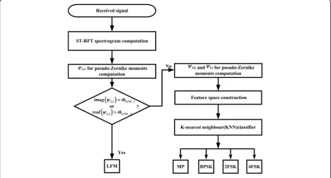
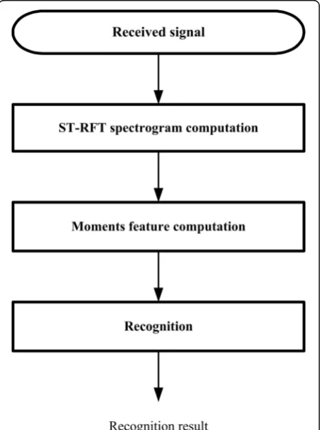
An intra-pulse modulation recognition approach based on Short-Time Ramanujan Fourier Transform (ST-RFT) and pseudo-Zernike moments feature is proposed in this paper. The system model of the proposed approach is shown in Fig. 1.

Three parts are included in this research: ST-RFT spec-trogram computation, moments feature computation, and recognition. The ST-RFT analysis is a preprocess of mo-ments feature computation, which could be used to obtain the ST-RFT spectrograms so as to represent features of intra-pulse modulation signals under negative SNR.

In the moments feature computation part, pseudo-Zernike moments features selected based on the degree of overlapping between each pair of classes of the signal data set are extracted from the spectrograms for its good invariance properties, which consist of ψ3,3 feature and

ψ2,0,ψ5,1features.

After ψ3,3 feature computation, intra-pulse modulation

signals are described by vectors. These describing vectors are used for recognition by using threshold decision. Fur-thermore, afterψ2,0 andψ5,1 features computation,

intra-pulse modulation signals are described by matrices, which are used for recognition by using KNN classifier [22].

3 Mathematical model of ST-RFT spectrogram and ST-RFT spectrogram features

3.1 Ramanujan Fourier transform (RFT)

In the classical DFT, the basis functionsep(n) are defined as [16] basis frequency (1/q).

In the RFT, Ramanujan sums(RS)cq(n) are sums defined as the n-th powers of q-th primitive roots of unity [23]

cqð Þ ¼n primitive characters ep(n). In other words, the basis functions are built by summing up components which are multiples of the same periodicityq, and only compo-nents satisfying (p,q) = 1 contribute to the sum.

The sums were introduced by Ramanujan to play the role of base functions over which typical arithmetical functionss(n) may be projected

s nð Þ ¼X ∞

q¼1

sqcqð Þn ð3Þ

It is obvious that an arithmetical functions(n) is an in-finite sequence defined for 1≤n≤ ∞for RFT, rather than that for DFT which is taken with a finitenshown in [24].

Thesqis referred to as the RFT coefficient given by [25]

sq¼

which is what we called the RFT.

Meanwhile, one can write the Wiener-Khintchine formula according to [26], and the linear property and the frequency multiplication property of RFT can be readily obtained.

3.2 ST-RFT spectrogram computation

In this paper, the ST-RFT is used to extract the neces-sary features of 5 modulations for intra-pulse modula-tion recognimodula-tion. The reasons for this choice is that as a windowed RFT function, the ST-RFT transform allows simultaneous description of a signal in time and fre-quency so that the temporal evolution of the signal spectrum can be analyzed in the time-frequency space.

For an arbitrary discrete-time signal s(n) of length N, the ST-RFT of the signal is defined as

ST−RFTsðk;qÞ ¼

whereφ(k) is the Rectangular window function of length H, andφ(0) = 1.

Then the ST-RFT spectrogram Ss(k,q) defined as the squared absolute value of the ST-RFT ofs(n) is given by

Ssðk;qÞ ¼jST−RFTsðk;qÞj2: ð6Þ

In the present work here, we take MP signal as an ex-ample to illustrate the deduction of the ST-RFT spectro-gram expression of 5 modulations: MP signal, LFM signal, BPSK signal, 2FSKsignal and 4FSK signal.

Considering the following continuous-time MP signal

sMPð Þ ¼t Aej2π

1

Ttþφ0

ð Þ_{; ð7Þ}

wherefcis the carrier frequency(CF),T ¼_f1

cis the period

of the continuous-time signal, A and φ0 are the

ampli-tude and the initial phase of MP separately.

For a sampling interval of Ts (the sampling frequency (SF) is f_s¼_T1_s), the discrete representation of signal (7)

Let us represent Ts

T as

whereT0represents the number of samples in one cycle

can be written asT0¼f_fs

Using Eq. (5), the ST-RFT of MP can be expressed as

ST−RFTMPðk;T0Þ ¼

Aej 2π −kþ1

ð Þ

T0 þφ0

ϕð ÞT0 ; ð

10Þ

in the case ofq=T0.

Substituting Eq. (10) into Eq. (6), the ST-RFT spectro-gram of MP becomes

SMPðk;T0Þ ¼jST−RFTMPðk;T0Þj2¼

A2

ϕð ÞT0

ð Þ2:

ð11Þ

3.3 ST-RFT spectrogram features

3.3.1 Analysis of ST-RFT spectrogram features

In practice, there exists a tradeoff between time and fre-quency resolution when determining the window length (the duration of window), that is to say, a long duration of window will provide a poor frequency resolution and vice versa. Through a series of simulation experiments, a

Rectangular window of length H¼4000

10 ¼400 is

selected, which can provide the best frequency

resolution-time resolution tradeoff for 5 modulations above-mentioned. Examples of amplitude normalized ST-RFT spectrograms Ps(k,q) (a normalization with

respect to its maximum value of each ST-RFT spectro-gram Ss(k,q))of 5 modulations computed from a sample of length N= 4000 with a Rectangular window of length

H= 400 are shown in Fig. 2a-e. The contours on the plot represent relative magnitude with the horizontal axis as q and the vertical axis ask(μs).

Figure 2 shows the amplitude normalized ST-RFT spectrograms Ps(k,q) reflecting time-frequency distribu-tion features of 5 types of moduladistribu-tion signals. Fig.2a shows the PMP(k,q) for MP signal. Ideally, there would be a straight line centred about T0 in k-q plane as the

Eq. (11) implied. By contrast, Fig. 2a shows the line to be spread out in q direction at the expense of reduced frequency resolution, and the peak energy is mainly con-centrated in the location of T0. The PLFM(k,q) for LFM

signal with chirp rate u= 300 as depicted in Fig.2b. Based on the observation of the spectrogram, the spectrum line can be approximated by a piecewise line starting at T0and finishing at T0−i,where i= 1, 2,…T0 −1, and each segment reflects the change of its fre-quency and phase. The PBPSK(k,q) for BPSK signal shown in Fig. 2c illustrates that the amplitude of spectrum obtains the minimum at instant of time of phase conversion, and in the duration of intercode, the

PBPSK(k,q) is the same as thePMP(k,q). The P2FSK(k,q)

for 2FSK signal can be seen in Fig. 2d, which has five vertical line segments centered about T0 and T1 in k-q

Fig. 2Examples of amplitude normalized ST-RFT spectrogramsPs(k,q) computed from a sample of lengthN= 4000 with a Rectangular window

of lengthH= 400 for 5 modulations: (a)PMP(k,q) for MP signal; (b)PLFM(k,q) for LFM signal; (c)PBPSK(k,q) for BPSK signal encoded by Barker codes;

plane embodying the number of frequency points, while for the P4FSK(k,q) of 4FSK signal has 5 ones centered

aboutT0,T2,T1,T0,T3in k-q plane as shown in Fig. 2e.

In summary, the contours on the plot show different spectrogram features of 5 modulations. Hence, the ST-RFT spectrograms can serve as a discriminating feature.

3.3.2 Analysis of discriminability

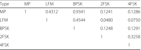
The parameter R giving the similarity degree between two amplitude normalized spectrogram Ps1(k,q) and Ps2(k,q) is defined as

The similarity degree is bounded, 0≤R≤1.

The similarity between any two amplitude normalized ST-RFT spectrograms computed by Eq. (12) with respect to different modulations in the absence of noise is depicted in Table 1. Intuitively, the MP and BPSK signals are difficult to distinguish from each other due to the fact that the spectrograms of the two modulations are similar enough with a similarity degree of 0.9341. In addition, for MP and LFM signals as well as LFM and

BPSK signals, the corresponding R are 0.4312 and

0.4544 respectively that means this feature is considered not reliable to provide an effective method of signal differentiation.

Furthermore, the theoretical analysis in Section 3.2 indicates that the location of the ST-RFT spectral peak will be shifted induced by the variation of CFs of the input signals, then alter the feature valuePs(k,q) and will finally influence the recognition results.

To tackle these problems, we propose a novel signal rec-ognition method that is based on the combination of the ST-RFT spectrogram and the pseudo-Zernike moments.

4 Mathematical model of pseudo-Zernike moments and moments feature selection 4.1 Mathematical model of pseudo-Zernike moments Moments have been widely used in image processing for pattern recognition due to its useful invariance properties such as translation, scale, and rotational invariance [21, 27]. Such features capture global information about the image and do not require closed boundaries as boundary-based methods such as Fourier descriptors [27].

The formation of polar coordinates of the pseudo-Zernike moments for f(x,y) can be obtained by project-ing f(x,y) onto orthogonal pseudo-Zernike polynomials

Re,m(ρ)eieθ, by the integral [28]. counterclockwise angular displacement in radians from the positive x -axis. Re,m(ρ) are the radial polynomials

expressed as represents its angular dependence, which takes on posi-tive and negaposi-tive integer values subject toe≥|m| only.

4.2 The translation invariance of pseudo-Zernike moments The translation invariance [27] of the pseudo-Zernike moments is suitable to be applied in illustrating effects of the variation of CFs and is utilized as time-frequency spectrogram features in radar signal classification.

For the amplitude normalized spectrogramPs(k,q) of the 5 modulations, the translation invariance is done by trans-forming the original time-frequency spectrogram Ps(k,q) into another one which isPs kþk;qþq

, wherekandq

are the centroid location ofPs(k,q) computed from

k¼m10 m00;

q ¼m01

m00; ð

15Þ

where m00 is the zero order moment defined as m00

¼ X

In other words, the origin is moved to centroid before moment comoutation.

Table 1Similarity between twoPs(k,q) with respect to different

modulations in the absence of noise

Type MP LFM BPSK 2FSK 4FSK

MP 1 0.4312 0.9341 0.1241 0.1286

LFM 1 0.4544 0.0480 0.0750

BPSK 1 0.1248 0.1291

2FSK 1 0.3258

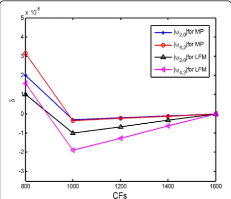
In the present work here, a parameter δ is presented to illustrate the translation invariance of the pseudo-Zernike moments is suitable to be applied in signal recognition when CFs change. are very small. Consequently, the features are nearly in-variant to CFs changing and are feasible for signal classi-fication with the variation in the signal CFs.

4.3 Pseudo-Zernike moments feature selection

The overlap measure indicates the degree of overlapping between two clusters, which can be quantified by com-puting an inter-cluster overlap [29]. A definition of the overlap rate(OLR) was proposed in [30], which is utilized as representative of the degree of overlap between the given two clustersCiand Cj. The OLR is determined by the ratio of the number of the overlap points to that the number of small cluster’s points.

OLR Ci;Cj

whereNOver_Region represents the number of the overlap points,Nmin is the minimum value of Ni and Nj, which stands for the number of points in each cluster

separately. TheOLR(Ci,Cj) varies from 0 to1, the closer the OLR(Ci,Cj) is to 0, the better the cluster separation is. Conversely, the closer theOLR(Ci,Cj) is to 1, the two clusters become more strongly overlapped.

In the following, three pseudo-Zernike moment features based on the average value of OLR(OLR′)are proposed for signal recognition. Here the signal data projected onto the 2-D/4-D feature space is obtained by testing all features of the pseudo-Zernike moments ran-ging from order 1 to order 6.

The algorithm of the moments feature selection for distinguishing LFM with the time-bandwidth between 8 and 500 in the case of SNR varying from -5 dB to 5 dB from the rest of signals is summarized as follows:

step 4: Combining the advantages of imag(ψ3,3) and real(ψ3,3) to discriminate LFM signals with large

vari-ation range in the time-bandwidth product from other modulations.

For other signals classification, we tested all combina-tions of two features ranging from order 1 to order 6

and measured the OLR′¼

X

OLR

6 which is defined as

the average value of OLR between different classes taken in the 4-D feature space and find the minimum. Follow-ing the foresaid algorithm, the 8th order moments of index 5 versus index27 for pseudo-Zernike moments

Fig. 3The values ofδversus different CFs of MP and LFM withu= 80

Algorithmmoments feature selection for LFM signal distinction 8≤uτ2≤500

Input:s{MP,BPSK,LFM, 2FSK, 4FSK}

1.RepeatforL= 1, 2,...50 (update the simulation times) 2. UpdatePð Þ_siL_;d;uτ2 kþk;qþq

ð Þand the corresponding

imag(L)(_ψe,m)

ð Þand the corresponding

real(L)(ψe,m) 9.end if

referring to ψ2,0 and ψ5,1 are experimentally selected as

features, which specifically suitable for signal classifica-tion with the excepclassifica-tion of LFM.

Theψ2,0andψ5,1are given by

ψ2;0¼

3

π Z

0 2πZ 1

0

R2;0ð ÞPρ ~sðρcosθ;ρsinθÞρdρdθ;

ð19Þ

ψ5;1¼

6

π Z

0 2πZ 1

0

R5;1ð Þeρ −iθP~sðρcosθ;ρsinθÞρdρdθ;

ð20Þ

R2;0ð Þ ¼ρ 10ρ2−12ρþ2; R5;1ð Þ ¼ρ 330ρ5−840ρ4

þ756ρ3−280ρ2þ35ρ:

5 Recognition algorithm 5.1 Steps of the proposed algorithm

The proposed modulation signal recognition algorithm is shown in Fig. 4.

The starting point are the modulation signals ~s nð Þ;n

¼0;1;…;N−1 to which Gaussian white noise is added. And the following steps of classifying various modula-tion types of signals are shown as follows:

Step 1: ST-RFT spectrogram Computation.

Step 1.1 Computing the amplitude normalized ST-RFT spectrogramP~sðk;qÞof 5 modulations mentioned-above.

Step 1.2 Computing the centroid moved amplitude normalized ST-RFT spectrogramP~s kþk;qþq

. Step 2: LFM signal classification.

Measuring imag(ψ3,3) and real(ψ3,3) respectively. If imag(ψ3,3) >thLFM_1 or real(ψ3,3) <thLFM_2, the signal is

regarded as LFM, else go to step 3. Step 3: Other signals classification.

Step 3.1 Pseudo-Zernike moments ψ2,0 and ψ5,1

computation.

Step 3.2 Constructing the 2-D feature space by using ψ2,0 and ψ5,1 and determining the optimal distribution

range of the spectrogram features of different modula-tions from the feature space.

Step 4: Use a K-nearest neighbour(KNN)classifier to assign each element to a class for the input radar signals, to perform the classification procedure.

5.2 The thresholds for LFM signals recognition

The thresholds thLFM_1 and thLFM_2 are utilized to

distinguish LFM with the time-bandwidth product between 8 and 40 and to distinguish LFM with the time-bandwidth product between 41 and 500 from other signals. They could be obtained by the iterative thresh-olding algorithm [20] and lots of simulations.

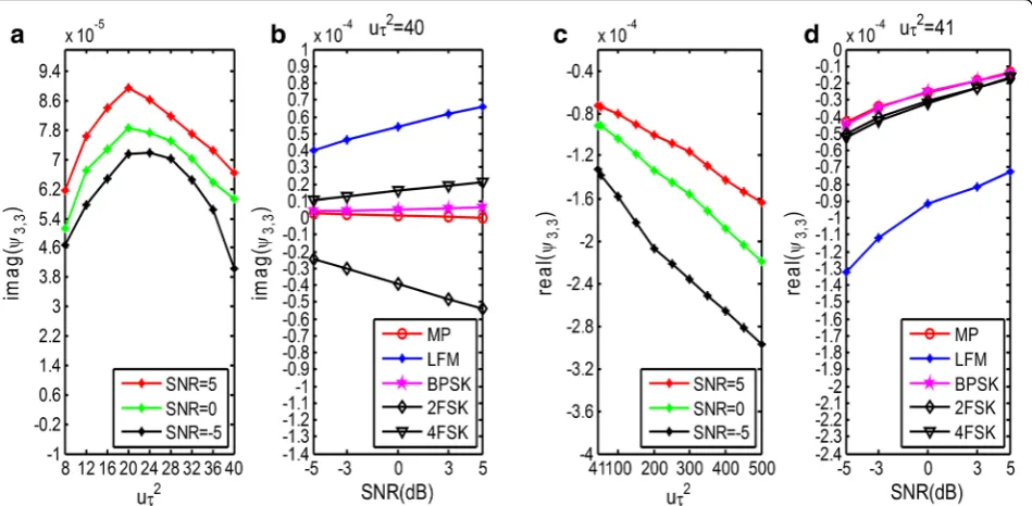
As in Fig. 5a, the minimum of the average value of

imag(ψ3,3) for LFM signal class is obtained when uτ2=

40 atSNR=−5dB which is close to 0.40 × 10−4and for the rest of other signal classes the maximum of the aver-age value ofimag(ψ3,3) obtained atSNR= 5dBis close to

0.21 × 10−4in general as shown in Fig. 5b. Finally, we set

thLFM1¼

0:4010−4_þ0:2110−4

2 ¼0:3110−

4 _{as the optimal}

threshold for LFM classification. Meanwhile, as in Fig. 5c, the average value of real(ψ3,3) for LFM signal class

ob-tains the maximum at uτ2= 41 for SNR = 5 dB and the maximum is close to−0.73 × 10−4, and for other signal classes, the minimum of the average values of real(ψ3,3)

is close to −0.50 × 10−4 obtained at SNR=−5dB from

Fig. 5d. Thus the threshold thLFM_2 can be set to

−0:7310−4_þ−0:5010−4

2 ¼−0:6210−

4 _{to guarantee the}

correct classification of the LFM signals with the time-bandwidth product between 41 and 500.

6 Results and discussion

6.1 Choice of the modulation signal parameters for the Clustering

The parameters used for the clustering are shown in Table 2. CR, PW and HS stand for code rate, pulse-width and frequency hop size, respectively. Meanwhile, for BPSK, we use 5 bit Barker codes, the 2FSK and 4FSK are encoded by deterministic codes in order to lower the

effect of deficiency of some codes. Codes are defined as [0 1 0 1 0] for 2FSK and [0 1 2 3 0]for 4FSK. And the length of Rectangular window is set to be 400. In addition, the SNR values from -5 to 5 dB for most conditions.

6.2 Choice of the modulation signal parameters for test In order to verify that the proposed method can achieve better performance than the algorithm based STFT, we did the following simulations. The code parameters for

BPSK、2FSK and 4FSK are same as the parameters set

in 6.1 for both algorithms. The CFs are 800 MHz, 1000 MHz and 1600 MHz. The HSs are 60 MHz, 100 MHz and 1000 MHz. The chirp rates for LFM are

40 MHz/ μs,80 MHz/ μs,100 MHz/ μs,1200 MHz/

μs.And the length of rectangular window is set to be 400 and the SNR values from -5 to 5 dB.

6.3 Simulation results analysis

To estimate the classifier performance, 50 signals are used for the clustering, and each simulation was run 100 times, evaluating the average recognition rate (ARR).

6.3.1 The effects of CFs and HSs variation

Figure 6 is used to get indications how much the CFs and HSs variation affect the performance at SNR = 5 dB

and SNR = 0 dB respectively. The MP、BPSK and LFM

signals are simulated with CFs ranging from 800 MHz to 1600 MHz, the FSK signals are simulated with HSs ran-ging from 60 MHz to 1000 MHz. As expected, the vari-ation in CFs and HSs would not affect the performance

Fig. 5The thresholds for LFM signals recognition:athe average values ofimag(_ψ3,3) against differentuτ2ranging from 8 to40 for different SNR

values;bthe average values ofimag(_ψ3,3) versus SNR for different modulations foruτ2= 40;cthe average values ofreal(ψ3,3) against differentuτ2

ranging from 41 to500for different SNR values;dthe average values ofreal(_ψ3,3) versus SNR for different kinds of signals foruτ2= 41

Table 2Parameters for the clustering

Signal type CF CR PW HS

MP 800 MHz 1μs

BPSK 800 MHz 10 MHz/μs 1μs

2FSK 800 MHz 10 MHz/μs 1μs 100 MHz

much. And the property makes the pseudo-Zernike moments very suitable to spectrogram features recognization with random variation in the signal parameters: CFs and HSs.

6.3.2 The performance of the proposed algorithm

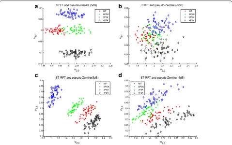
Figure 7 reports the scatter plots related toψ2,0 and ψ5,1

for pseudo-Zernike for all the data of the 4 types modula-tion signals for different SNR. Both the STFT and ST-RFT

based algorithms have been considered. The scatter plots shown in Fig. 7a and c demonstrate that for SNR = 5 dB, the extraction of the pseudo-Zernike moments from ST-RFT give a certain degree of separation within the class. As shown in Fig. 7b and d, for SNR = -5 dB the 4 classes could be considered to be classified more accurate by the proposed algorithms in comparison to the STFT based al-gorithm. Consequently, in the presence of noise, the

Fig. 6The effects of CFs and HSs variation: (a) Performance analysis for different CFs for MP、BPSK and LFM signals atSNR= 5dB; (b) Performance analysis for different HSs for FSK signals atSNR= 0dB

proposed algorithm performs well especially for MP and BPSK signals recognition.

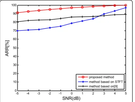
These behaviors are also confirmed by the results illus-trated in Fig. 8, where the ARR is plotted versus different SNRs ranging from -5 dB to 5 dB both for STFT, ST-RFT based algorithms and the algorithm presented in [9]. Thereinto, for STFT and ST-RFT algorithms, the modulations used to obtain the ARR are MP, LFM, BPSK, 2FSK and 4FSK signals satisfying the signal parameters for test discussed in the paper. And for [9], the modulations used to obtain the ARR are the signals of their own choosing. It is obvious that, an increment in the SNR leads to a higher performance. Obviously, in the case of SNR = -5 dB, the proposed algorithm reaches a ARR of 90%, while the ARR of STFT algorithm reaches 70%,and the ST-RFT based algorithms assure a higher level of ARR than the STFT counterpart. Consequently, as conclusion to these analyses, it can be claimed that the performance of our algorithm based on the combin-ation of the ST-RFT and the pseudo-Zernike moments is preferred to STFT based algorithm. Meanwhile, com-parison of the work to the techniques presented in [9] shows that the approach proposed in this paper has better robustness against SNR variation.

7 Conclusions

In this paper, we have presented a new method for intra-pulse modulation recognition under low SNR environ-ment. In this method, the ST-RFT spectrograms for 5 modulation schemes are firstly calculated. Then the pseudo-Zernike moments are applied to the ST-RFT spectrogram to uniquely discriminate the spectrogram features for different modulations when parameters change. Simulation results demonstrate a robust recog-nition performance over a wide range of SNRs, CFs, HSs, and time-bandwidth product. Meanwhile, based on

the simulation results analysis, our method is better comparison of the work to the STFT based technique and the technique presented in [9].

However, our work only on few modulation schemes, a discussion on the technique applied to other modulation schemes, such as NLFM, PWM, PPM will be developed.

Abbreviations

2D:Two-dimensional; 2FSK: Binary frequency shift keying; 4FSK: 4-ary frequency shift keying; ASK: Amplitude shift keying; ARR: Average recognition rate; BPSK: Binary phase shift keying; CF: Carrier frequency; CR: Code rate; DFT: Discrete Fourier Transform; FB: Feature based; FSK: Frequency shift keying; GCD: Greatest common divisor; HS: Hop size; HT: Hough transform; KNN: K-nearest neighbour; LFM: Linear frequency modulation;

MP: Monopulse; M-PSK: M-ary phase shift keying; OLR: Overlap rate; PW: Pulse-width; PSK: Phase shift keying; PSR: Probability of successful recognition; QPSK: Quadrature phase shift keying; RS: Ramanujan sums; RFT: Ramanujan Fourier Transform; STFT: Short-time Fourier transform; ST-RFT: Short-Time Ramanujan Fourier Transform; SF: Sampling frequency; SNR: Signal-to-noise ratio; WVD: Wigner_–Ville distribution

Acknowledgements

The authors would like to thank the reviewers for their time and effort spent in carefully reviewing the manuscript, and for their valuable comments that have greatly contributed to the enhancement of article’s quality.

Funding

This work is partially supported by Tianjin Research Program Application Foundation and Advanced Technology (15JCQNJC01100).

Authors’contributions

XM conceived the approach; XM, DL and YS designed the experiments; DL and YS performed the experiments. All authors read and approved the final manuscript.

Competing interests

The authors declare that they have no competing interests.

Publisher

’

s Note

Springer Nature remains neutral with regard to jurisdictional claims in published maps and institutional affiliations.

Received: 3 December 2016 Accepted: 24 April 2017

References

1. W Pei, QZ Yang, Z Jun, T Bin, Autonomous radar pulse modulation classification using modulation components analysis. EURASIP J. Adv. Signal Process. 2016(1), 1-11(2016)

2. OA Dobre, A Abdi, Y Bar-Ness, W Su, Survey of automatic modulation classification techniques: classical approaches and new trends. IET Com

1(2), 137–156 (2007)

3. D Grimaldi, S Rapuano, LD Vito, An Automatic Digital Modulation Classifier for Measurement on Telecommunication Networks. IEEE Trans Instrum Meas

56(5), 1171–1720 (2007)

4. SZ Hsue, SS Soliman, Automatic modulation classification using zero crossing. IEE Proc, Radar, Sonar Navig137(6), 459–464 (1990) 5. H Alharbi, S Mobien, S Alshebeili, F Alturki, Automatic modulation

classification of digital modulations in presence of HF noise. EURASIP J Adv Signal Process1, 3639–3654 (2012)

6. K Hassan, I Dayoub, W Hamouda, M Berbineau, Automatic Modulation Recognition Using Wavelet Transform and Neural Networks in Wireless Systems. EURASIP J Adv Signal Process1, 1–13 (2010)

7. S Qian, D Chen, Joint Time-Frequency Analysis. IEEE Sig Process Mag

16(2), 52–67 (1999)

8. F Hlawatsch, GF Boudreaux-Bartels, Linear and quadratic time-frequency signal representations. IEEE Sig Process Mag9(2), 21–67 (1992)

9. Z Yang, W Qiu, H Sun, A Nallanathan, Robust Radar Emitter Recognition Based on the Three-Dimensional Distribution Feature and Transfer Learning. Sensors16(3), 1–14 (2016)

10. G Lopez-Risueno, J Grajal, A Sanz-Osorio, Digital Channelized Receiver Based on Time-Frequency Analysis for Signal Interception. IEEE Trans Aerosp Electron Syst41(3), 879_–898 (2005)

11. Y Zhang, X Ma, D Cao, Automatic Modulation Recognition Based on Morphological Operations. Circuits Syst Signal Process32(5), 2517–2515 (2013) 12. D Zeng, H Xiong, J Wang, B Tang, An Approach to Intra-Pulse Modulation

Recognition Based on the Ambiguity Function. Circuits Syst Signal Process

29(6), 1103–1122 (2010)

13. D Zeng, X Zeng, H Cheng, B Tang, Automatic modulation classification of radar signals using the Rihaczek distribution and Hough transform. IET Radar Sonar Navig6(5), 322_–331 (2012)

14. TJ Lynn, AZ Sha’amerr,Automatic analysis and classification of digital modulation signals using spectrogram time frequency analysis.Proc. International Symposium on Communications & Information Technologies (CIT'07) (,Sydney, NSW,2007), pp. 916-920.

15. F Xie, C Li, G Wan,An Efficient and Simple Method of MPSK Modulation Classification. 4th International Conf. on Wireless Communications, Networking and Mobile Computing (WiCOM '08) (,Dilian, China, 2008), pp. 1–3

16. M Planat, H Rosu, S Perrine, Ramanujan sums for signal processing of low-frequency noise. Phys Rev E66(5), 715–720 (2002)

17. LT Mainardi, L Pattini, S Cerutti, Application of the Ramanujan Fourier Transform for the Analysis of Secondary Structure Content in Amino Acid Sequences. Meth Inf Med46(2), 126_–129 (2007)

18. S Samadi, MO Ahmad, MNS Swamy, Ramanujan Sums and Discrete Fourier Transforms. IEEE Signal Process Lett12(4), 293–296 (2005)

19. L Sugavaneswaran, S Xie, K Umapathy, S Krishnan, Time-Frequency Analysis via Ramanujan Sums. IEEE Signal Process Lett19(6), 352_–355 (2012) 20. J Lundén, V Koivunen, Automatic Radar Waveform Recognition, IEEE Journal

of selected topics in signal process.1(1), 124-126 (2007)

21. C Clemente, L Pallotta, AD Maio, JJ Soraghanand, A Fatina, A Novel, Algorithm for Radar Classification Based on Doppler Characteristics Exploiting Orthogonal Pseudo-Zernike Polynomials. IEEE Trans Aerosp Electron Syst51(1), 417–430 (2015)

22. MW Aslam, Z Zhu, AK Nandi, Automatic Modulation Classification Using Combination of Genetic Programming and KNN. IEEE Trans Wireless Commun11(11), 2742–2750 (2012)

23. S Ramanujan, On certain trigonometric sums and their applications in the theory of numbers. Trans Cambridge Philos Soc22(13), 259–276 (1918) 24. PP Vaidyanathan, Ramanujan Sums in the Context of Signal

Processing—Part I: Fundamentals. IEEE Trans on Signal Process

62(16), 4145–4157 (2014)

25. RD Carmichael, Expansions of arthmetical functions in infinite series. Proc London Math Soc34(13), 1_–26 (1930)

26. M Planat, M Minarovjech, M Saniga, Ramanujan sums analysis of long-period sequences and 1/f noise. Epl85(4), 4005–4010 (2008)

27. A Khotanzad, YH Hong, Invariant Image Recognition by Zernike Moments. IEEE Trans Pattern Anal Mach Intell12(5), 489_–497 (1990)

28. R Mukundan, KR Ramakrishnan,Moment Functions in Image Analysis- Theory and Applications(River Edge, NJ, 1998), pp. 1-150

29. K Dae-Won, KH Lee, D Lee, On cluster validity index for estimation of the optimal number of fuzzy clusters. Patt Recog37(10), 2009_–2025 (2004) 30. Z Hong, Q Jiang, H Guan, F Weng,Measuring overlap-rate in hierarchical

cluster merging for image segmentation and ship detection. Proc. International Conference on Fuzzy Systems & Knowledge Discovery(FSKD'07) (,Haikou, Hainan, China, 2007), pp. 420-425

Submit your manuscript to a

journal and benefi t from:

7 Convenient online submission 7 Rigorous peer review

7 Immediate publication on acceptance 7 Open access: articles freely available online 7 High visibility within the fi eld

7 Retaining the copyright to your article